Relativistic corrections to double B_c meson production in e⁺e^– annihilation

Heavy quarkonia and the $ B_c $ meson, which are bound states of heavy quark pairs ($ c\bar{c} $, $ b\bar{b} $, $ c\bar{b} $, and $ b\bar{c} $), serve as excellent probes for testing quantum chromodynamics (QCD) and the standard model (SM). Their theoretical description is facilitated by nonrelativistic QCD (NRQCD) factorization formalism [1], which is available because of the large heavy quark mass and small relative velocity between $ Q\bar{Q} $ (or $ Q\bar{Q}' $). The pair production of heavy quarkonia in $ e^+e^- $ annihilation provides a crucial testing ground for NRQCD. To match experimental data, both QCD and relativistic corrections are essential [2–9]. Given that $ v^2 \sim \alpha_s $, these two types of corrections are expected to be comparable in magnitude. Motivated by proposed future high-luminosity $ e^+e^- $ colliders such as the circular electron positron collider (CEPC) [10], future circular collidor electron-positron [11], or Z-factory [12], the leading order (LO) and next-to-leading order (NLO) QCD corrections for double heavy quarkonia production at the $ Z^0 $ peak have been computed [13–20]. These studies indicate promising detection prospects and reveal that the contributions from color-octet (CO) components and relativistic corrections are also significant [20].

The $ B_c $ meson stands out in the heavy quark bound states family because of its composition of different-flavor quarks and unique weak decay mode. These characteristics provide clearer insights into decay and production mechanisms than those with other quarkonia. Thus far, the only observed $ (b\bar{c}) $ state is the ground state $ B_c^+(1S) $, first discovered at the Tevatron in 1998 [21, 22] and later confirmed by large hardon collider (LHC) experiments [23–27], and its excited state $ B_c^+(2S) $, discovered approximately 15 years later by the ATLAS [28], CMS [29], and LHCb collaborations [30]. Theoretically, $ B_c $ production has been extensively studied across various collision processes. These include direct production in $ e^+e^- $ annihilation (electron production)[31–37] and $ \gamma\gamma $ fusion (photon production) [38–45] at ee colliders; $ gg $ fusion (hadron production) at hadron colliders [41, 46–51]; $ \gamma g $ fusion (lepton-hadron production) at $ ep $ colliders [52, 53]; production in heavy-ion collisions Pb+Pb at the LHC [54, 55]; and indirect production via the decays of heavy particles such as the W, Z, and Higgs bosons, as well as the top quark [56–66].

The electron-positron production of paired $ B_c $ mesons has been calculated with the collinear factorisation [67]. The LO cross section [17–19, 68], NLO QCD corrections[69] with NRQCD approach, and the relativistic corrections to both the s-channel single-photon [70] and t-channel double-photon exchange processes [71] within the relativistic quark model (RQM) have been investigated. However, in contrast to the extensive studies on QCD corrections to $ B_c $ production or the QCD and relativistic corrections to charmonium and bottomonium production, relativistic effects in processes involving $ B_c $ mesons have received comparatively little attention [43, 65, 66, 70–81]. Most existing studies are based on the RQM [43, 65, 66, 70–74, 76], which incorporates relativistic corrections in the amplitude for the heavy quarks' relative motion and in the bound-state wave function. Given that the binding effects are significantly enhanced in pair meson production, we investigate the relativistic corrections for double $ B_c $ production in $ e^+e^- $ annihilation via both $ \gamma^* $ and $ Z^0 $ propagators within the NRQCD framework. The specific processes considered are: $ B_c^{*+}+B_{c}^{*-}, \ B_c^{*+}+B_{c}^{-}, \ B_c^{+}+ B_{c}^{-}$, $B_c^{*+}+h_{bc}^{-}, \ B_c^{*+}+\chi_{bc0}^{-}, \ B_c^{*+}+\chi_{bc1}^{-}$, $B_c^{*+}+\chi_{bc2}^{-},\ B_c^{+}+h_{bc}^{-}$, $B_c^{+}+ \chi_{bc0}^{-}, \ B_c^{+}+ \chi_{bc1}^{-}, \ B_c^{+}+\chi_{bc2}^{-} $ ¹.

The remainder of the paper is organised as follows. In Sec. II, we describe the theoretical framework for the NLO($ v^2 $) NRQCD calculations. In Sec. III, we present the input parameters used in this work. In Sec. IV, we show the results of the cross-sections, differential cross-sections, and azimuthal asymmetry with and without relativistic corrections. Finally, a brief conclusion is provided in Sec. V.

Within the NRQCD framework and up-to $ {\cal{O}}(v^2) $, the production cross-sections are factorized as [1]

where $ n_1,n_2 $ represent the Fock states denoted in spectroscopic notation $ {}^{2S+1}L_J^{[a]} $, with total spin S, orbital angular momentum L, total angular momentum J, and color configurations a = 1, 8 corresponding to color-singlet (CS) and CO states, respectively. m represents the heavy quark effective mass. $ {\cal{O}}^H(n) $ and $ {\cal{P}}^H(n) $ are four-fermion operators of mass dimensions $ d_{\cal{O}} $ and $ d_{\cal{P}} $ describing the nonperturbative transition $ n\rightarrow H $ at LO and $ {\cal{O}}(v^2) $. $ \langle{\cal{O}}^H(n)\rangle $ and $ \langle{\cal{P}}^H(n)\rangle $ are the respective long-distance matrix elements (LDMEs), and $ F(n_1,n_2) $ and $ G_i(n_1,n_2) $ are the appropriate short-distance-coefficients (SDCs). The SDCs describe the short-distance production of two Fock states $ (c\bar{b})[n_1] $ and $ (b\bar{c})[n_2] $, and the LDMEs describe the hadronization of the Fock state $ n_{1,2} $ into the physical $ B_c $ mesons $ H_{1,2} $. The SDCs are perturbatively calculable and the LDMEs can be obtained by the potential model [82–84] and potential NRQCD [85].

In the subsequent discussion, we see that the contribution of the CO channels for double $ B_c $ production is negligible compared to that of the CS channels. Within the CS framework, the relevant four-quark operators for the production of $ H=B_c, B_c^*,\cdots $ are defined as [1] (for simplicity, only the S-wave operators are listed herein).

where $ \psi(\chi) $ represents the Pauli spinor that annihilates (creates) a heavy quark (antiquark), $ {\boldsymbol{\sigma}}^i(i=1,2,3) $ are the Pauli matrices, and $ \overleftrightarrow{{\boldsymbol{D}}}=\overleftarrow{{\boldsymbol{D}}}-\overrightarrow{{\boldsymbol{D}}} $, with $ \overrightarrow{{\boldsymbol{D}}} $ being the space component of the covariant derivative $ D^\mu $.

For S and P wave states, the LDMEs at LO are related to the values of radial functions and the first derivatives of radial functions at the origin,

It is convenient to define matrix elements $ \langle v^2\rangle $ instead of the LDMEs at $ {\cal{O}}(v^2) $ [86–88].

The SDCs can be obtained via the matching condition between perturbative QCD and NRQCD calculations.

The left-hand side of Eq. (5) can be computed easily by using the covariant projection method [86].

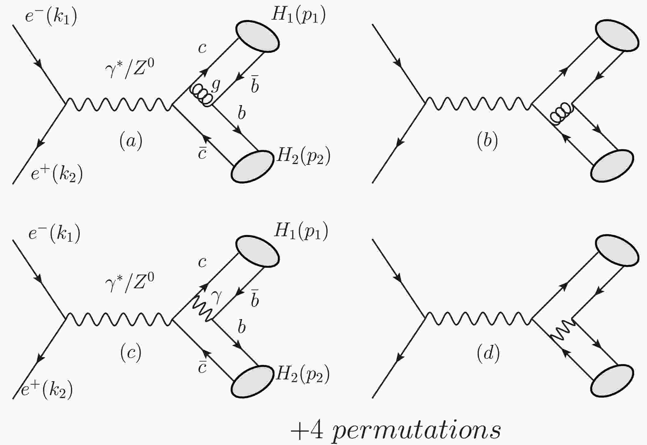
The Feynman diagrams for the exclusive $ B_c $ pair production $ e^-e^+ \to \gamma^*/Z^0 \to H_1^+(p_1) + H_2^-(p_2) $ are displayed in Fig. 1. Here, we only present diagrams for s-channel processes. The t-channel double-photon fragmentation mechanism dominates the production of $ J/\psi $ and $\Upsilon $ pairs [20, 89, 90], as the photon can fragment into a $ {}^3S_1 $ quarkonium state. In contrast, similar to the case of $ \eta_{c/b} $ pair production where the photon cannot fragment into a $ {}^1S_0 $ state because of C-parity conservation, that of the $ B_c $ pair production proceeds only via the non-fragmentation mechanism because a photon cannot fragment into a $ c\bar{b} $ quark pair. Subsequent calculations indicate that the t-channel contributions are negligible. In the diagrams, $ H_1 $ and $ H_2 $ are the positively and negatively charged $ B_c $ mesons, with the quark contents of $ c(p_c)\bar{b}(p_{\bar{b}}) $ and $ b(p_b)\bar{c}(p_{\bar{c}}) $, respectively. The momenta of the heavy quarks in the mesons are defined as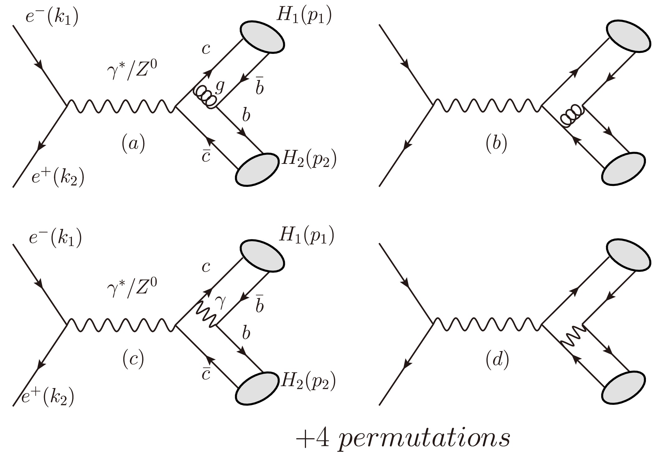

Figure 1.  Feynman diagrams for $ e^-(k_1)+e^+(k_2)\rightarrow \gamma^*/Z^0\rightarrow H_1(p_1)+ $$ H_2(p_2) $ at the tree level. $ H_1, H_2 $ are $ B_c^+(c\bar{b}) $ and $ B_c^-(b\bar{c}) $ (or their respective excited states, $ B_c^{*\pm}, h_{bc}^{\pm}, \chi_{bcJ}^{\pm} (J=0,1,2) $), respectively. The permutation diagrams can be obtained by reversing the quark lines and exchanging $ b,c $ quarks. (a) and (b) diagrams belonging to QCD channels, (c) and (d) diagrams belonging to EW channels.

$ \; E_{c/\bar{b}}=\sqrt{m_{c/b}^2+\vec{q}_1^2} $ and $ E_{b/\bar{c}}=\sqrt{m_{b/c}^2+\vec{q}_2^2} $ are the energies of constituent quarks in the rest frame of the meson, where $ \vec{q}_i(i=1,2) $ represent the three-momenta of the quarks; each can be expressed as the product of the reduced mass $ \mu_{H}=\dfrac{m_cm_b}{m_c+m_b} $ and effective quark velocity $ \vec{v} $. Meanwhile, $ q_{i} $ represents the corresponding four-momenta subject to constraints $ q_i\cdot p_i=0 $.

The full QCD scattering amplitude may be written as

where $ {\cal{A}}(e^+e^-\rightarrow c+\bar{b}+b+\bar{c}) $ represents the standard Feynman amplitude. In addition, the Breit-Wigner formula is utilized for the $ Z^0 $ propagator within the amplitudes [13, 17–20], namely ${\cal{D}}_{\mu\nu}=\dfrac{-{\rm i}g_{\mu\nu}}{p^2-m_Z^2+{\rm i}m_Z\Gamma_Z}$. The covariant projector method is employed in the calculations [7, 20, 77–79, 81, 88, 91–94]. The projector operator for $ H_1 $ in the spin-triplet state is given by

with the Dirac spinors normalized as $ \bar{u}u=2\;m_c $ and $ -\bar{v}v=2\;m_b $. Here, $ \epsilon_{S_z} $ represents a unit spin polarization vector. For the spin-singlet state, the spin state $ |1 S_z \rangle $ is replaced by $ |0 0 \rangle $, and $ \not{\epsilon}_{S_z} $ is replaced by $ \gamma_5 $. The expression $ \langle 3, k; \bar{3}, l | 1 \rangle = \dfrac{\delta_{k l}}{\sqrt{N_c}} = \dfrac{{\bf{1}}_c}{\sqrt{N_c}} $ corresponds to the Clebsch-Gordan coefficient in the SU(3) color space, which projects the $ (b\bar{c}) $ pair onto the CS state $ |1\rangle $. Here, $ {\bf{1}}_c $ represents the unit color matrix and $ N_c $ denotes the number of colors in QCD. The projector operator for $ H_2 $ can be obtained by making the following replacements in Eq. (9): $ \bar{b}\rightarrow \bar{c} $, $ c\rightarrow b $, and $ m_c\leftrightarrow m_b $. The complete color factor for QCD diagrams (a, b) is $ \dfrac{N_c^2-1}{2N_c}=C_F $; pure EW diagrams (c, d), 1; and t-channel double photon exchange processes discussed in Sec. IV.A, 1.

To expand Eq. (8) as a double series in $ q_1 $ and $ q_2 $, it is convenient to define

where the factor $ \sqrt{m_i/E_i} $ compensates the relativistic normalization ² of the $ (bc)_i $ pair with $ m_1=m_2=2\mu_H, \ E_1= 2E_cE_{\bar{b}}/(E_c+E_{\bar{b}})$, $E_2=2E_bE_{\bar{c}}/(E_b+E_{\bar{c}}) $. Such that

Here, the subscript "0" means no derivatives of $ q_i $ to the amplitude.

For S-wave states, only even powers of $ q_i $ contribute in the expansion. The following replacement is adopted in our calculations [7, 91]:

with $ \Pi_i^{\mu\nu}=-g^{\mu\nu}+\dfrac{p_i^\mu p_i^\nu}{p_i^2} $. For P-wave states, only odd powers of $ q_i $ contribute. The corresponding replacements are given as [92–94]

where $ \epsilon_{L_z}(p_i) $ represents the orbital polarization vector of the P-wave meson. For the $ ^3S_1 $ and $ ^1P_1 $ states, because the total angular momentum polarization vector equals the spin or orbital polarization vector, the corresponding polarization sum relationships are expressed as

For $ ^3P_J $ states ($ J=0,1,2 $), spin and orbital polarization vectors couple to generate the specific total angular momentum polarization, which can be expressed as

Upon summing over $ J_z $, the relevant polarization sum relationships are listed below [95].

As for the kinematics, the Mandelstam variables are defined as

$ t, u $ depend on $ |\vec{q}_{i}|^2 $. We define $ t_0,u_0 $ as values at $ |\vec{q}_{i}|^2=0 $ (non-relativistic result); therefore, $ t, u $ are expanded up-to $ {\cal{O}}(v^2) $ as

where $ M=m_c+m_b $. The master formulas for the SDCs in the matching condition of Eq. (5) are given by

where $ |{\cal{M}}|^2 $,$ |N_i|^2 $ denote the amplitudes squared at $ {\cal{O}}(v^0) $ and $ {\cal{O}}(v^2) $, respectively. $ 1/(8s) $ is the flux factor $ 1/(2s) $ multiplied by the spin-average factor $ 1/4 $ for the initial electron-positron pair. $ {\rm d}\phi_2^{(0)} $ is the two-body phase space integral element at $ {\cal{O}}(v^0) $, and $ f_{ps}=-\dfrac{r}{m_cm_b(1-4r)} $ with $ r=(m_c+m_b)^2/s $ comes from the relativistic expansion to the phase space factor ³. The amplitudes squared are explicitly expressed as below

where the first and second rows of Eqs. (23)−(25) correspond to the production of double S-wave $ B_c $ mesons and ''S+P''-wave $ B_c $ mesons, respectively.

We use the following input parameters in the numerical calculations [96, 97]

$ m_c, m_b $ represent the masses of charm and bottom quark, respectively; $ m_Z,\; \Gamma_Z $ are the mass and width of $ Z^0 $ boson, respectively; and $ \theta_w $ is the Weinberg angle. The values of the square of the effective velocity $ v^2 $ are estimated using [97]

where $ \langle T\rangle $ represents the averaged kinematic energy of quark inside the $ B_c $ meson and is estimated as $0.35\; {\rm GeV}$, as reported in Ref. [98].

The values of the original wave functions have been reported in several Refs. [71, 83, 84, 97, 99]. Here, we use the set from Ref. [84],

The matrix elements $ \langle v^2\rangle $ adhere to the velocity power scaling rules and are of the order of $ v^2 $ as

The running of strong coupling constant is taken at one-loop accuracy,

with the active quark flavors $ n_f=3 $, $\Lambda_{\rm QCD}=251\; {\rm MeV}$, and $ \alpha_s(m_Z)=0.1184 $. In the subsequent calculations, we treat $ \alpha_s(\mu) $ as running with the collision energy $ \sqrt{s} $, and we additionally quantify the uncertainties associated with the renormalization scale variation.

Figure 1 shows the four types of processes, denoted as γ-γ, γ-g, Z-γ, and Z-g. These labels specify the nature of the two propagators in each process. The contributions from the pure electroweak (EW) diagrams ($ \gamma^* $/ $ Z^0 $-γ type) are several orders of magnitude smaller than those from the QCD ($ \gamma^* $/ $ Z^0 $-g type) diagrams. This suppression factors can be estimated by $ [Q_cQ_b\alpha/(C_F\alpha_s)]^2\sim 10^{-4} $, which arises from the coupling constants, charge of the heavy quark, and color factors. Thus, previous studies in Refs. [17–19, 69, 70] considered only QCD processes. Here, we do not show the results of the four types of processes (γ-γ, γ-g, Z-γ, and Z-g); instead, we classify them into two types, i.e., γ-propagated (γ-γ, γ-g) and $ Z^0 $-propagated (Z-γ, Z-g) processes. Consequently, we investigate the paired $ B_c $ production via $ \gamma^*/Z^0 $-propagators separately, as in Refs. [13, 17, 19], and we show the cross-sections as a function of the center-of-mass (c.m.) energy in Fig. 2. The γ-propagated processes are dominant in the low energy region, while the $ Z^0 $-propagated processes are dominant around the Z-factory energy region because of the resonance effect. Further, the interference between different mechanisms (e.g., fragmentation and nonfragmentation [100]) can sometimes cause destructive contributions. Moreover, we calculated the interference contributions and found they were moderate, with the ratio $ (\sigma_{\text{total}}-\sigma_{\gamma}-\sigma_{Z})/\sigma_{\text{total}} $ ranging from –5% to 5%. In the following sections, we only discuss the total results (the sum of both processes, including the interference).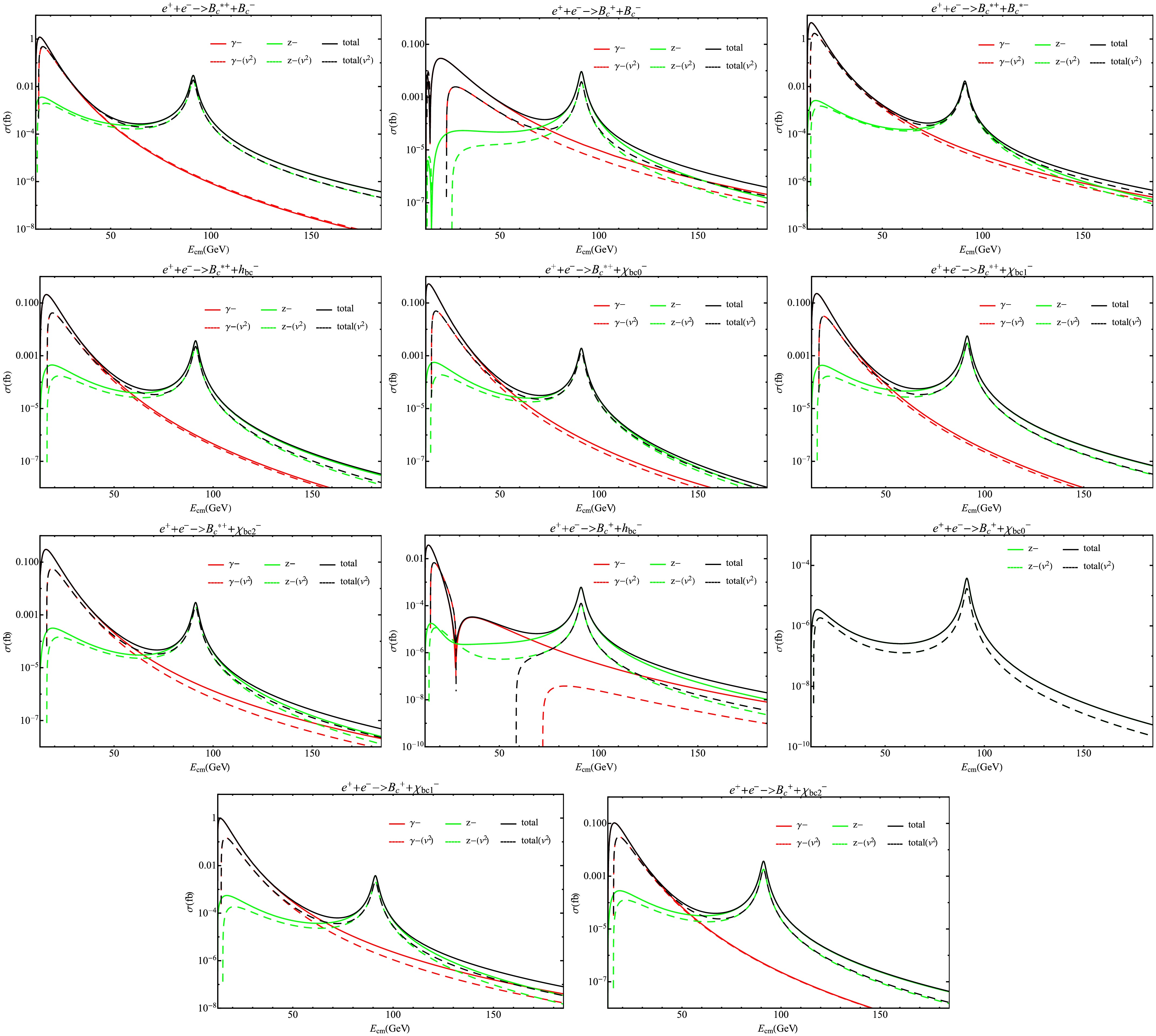

Figure 2.  (color online) Cross-section σ versus c.m. energy $ \sqrt{s}\; (E_{\rm cm}=\sqrt{s}) $. The red, green, and black lines correspond to γ-propagated processes, Z-propagated processes, and the sum of both, respectively. The solid line represents LO results, while the dashed line represents NLO($ v^2 $) results.

In contrast to Ref. [70], which studied the production of double S-wave $ B_c $ mesons via a virtual photon within the RQM, we present our results for the same mechanism within the NRQCD frame (s-channel γ-g type) in Fig. 3. The NRQCD method yields results are qualitatively consistent with those in the RQM calculations, i.e., the relativistic corrections have negative effects. The corresponding numerical cross-sections at $ \sqrt{s} = 22\ \text{GeV} $ are provided in Table 1.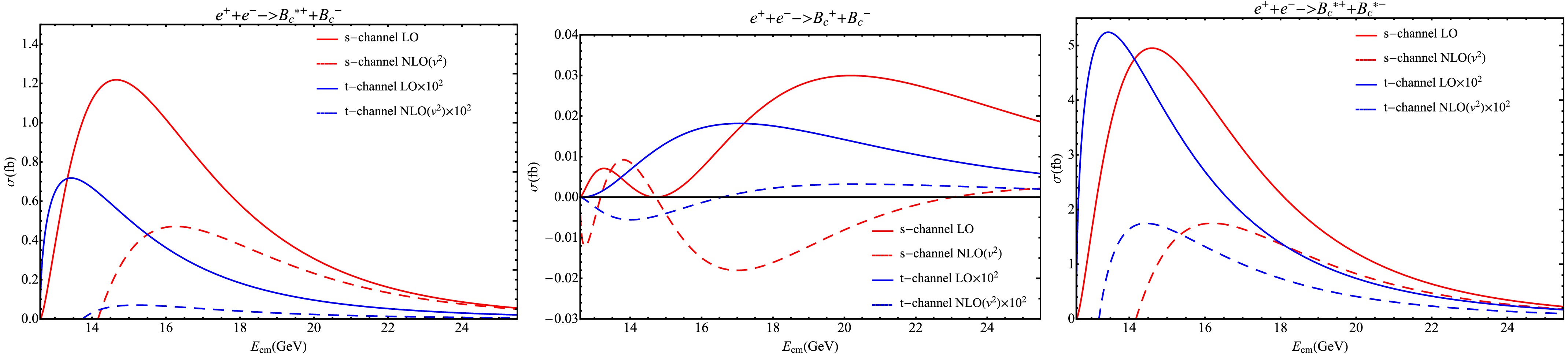

Figure 3.  (color online) Cross-section σ versus c.m. energy $ \sqrt{s}\; (E_{\rm cm}=\sqrt{s}) $ for the s-channel γ-g type and t-channel processes. The red and blue lines represent s-and t-channel processes, respectively. The solid and dashed lines represent LO and NLO($ v^2 $) results, respectively. The t-channel results are scaled up by a factor of 100.

The contributions of the t-channel double photon exchange have also been studied [71, 101]. We calculated the t-channel double photon production cross-sections and found that they were at least two orders of magnitude smaller than the corresponding s-channel cross-sections for all $ 11 $ processes considered herein. This is caused by a suppression factor of $ \alpha^2/\alpha_s^2 $ ($ \sim10^{-3} $). Therefore, these contributions can be safely neglected. However, for comparison with Ref. [71], which studied the t-channel double-photon production mechanism within the RQM, we present our relativistic results for t-channel processes within the NRQCD frame in Fig. 3. Similar to the RQM results of Ref. [71], our study demonstrates that relativistic effects lead to negative corrections. The remaining differences may originate from distinct theoretical frameworks and input parameters (e.g., quark masses and LDMEs). The numerical results at $ \sqrt{s} = 22 $ GeV are presented in Table 1.

Furthermore, for $ B_c^{+}+B_c^{-} $ production, Ref. [69] proposed that higher-order contributions such as two-loop QCD corrections or relativistic corrections may resolve the problem of negative cross-sections observed in the next-to-leading order (NLO) QCD calculations. However, Fig. 3 shows that this issue persists even when relativistic corrections are included. Additionally, interferences between s- and t-channels were calculated and failed to resolve the problem.

The numerical results of cross sections for all processes are presented in Table 2, in which we list the cross sections for different renormalization scales at three energy points ($ m_Z/2, m_Z, 2m_Z $), for both LO and NLO in $ v^2 $ expansions. The LO results are consistent with that in Ref. [69] when using the same input parameters ⁴. For $ B_c^{+}+B_c^{-} $ production via the γ-propagator, the LO cross section takes a zero at an energy point $ s_0 $ near the threshold or in the low energy region ⁵, and the value of $ s_0 $ is obtained as follows,

where $ r_c=m_c/M $, $ M=m_c+m_b $, which is consistent with Ref. [69]. In contrast, for $ B_c^{+}+h_{bc}^{-} $ production (via the γ-propagator), the LO cross-section at $\sqrt{s}\simeq28.0\; {\rm GeV}$ is not strictly zero ($\simeq1.3\times10^{-7}\;{\rm fb}$).

To examine the effects of the relativistic corrections, we plot the ratio $ \sigma_{\text{NLO}(v^2)}/\sigma_{\text{LO}} $ (i.e., the K-factors) as a function of the collision energy in Fig. 4. Compared to the NLO QCD cross-sections, for which the K-factors are about $ 1.2-2.0 $ [69], the K-factors for the relativistic corrections are about $ 0.2-1.0 $. At high energies, the relativistic K-factors are ~$ 0.6 $, indicating that relativistic corrections reduce the $ {\cal{O}}(v^0) $ cross-sections by about 40%. This level of suppression is expected and reasonable because it lies between the ~50% reduction calculated for double charmonia production and ~20% reduction for double bottomonia production [20]. In Appendix A, we present the ratios of the relativistic corrections to the LO SDCs in the high-energy limit, which also reflect the contributions of the relativistic corrections.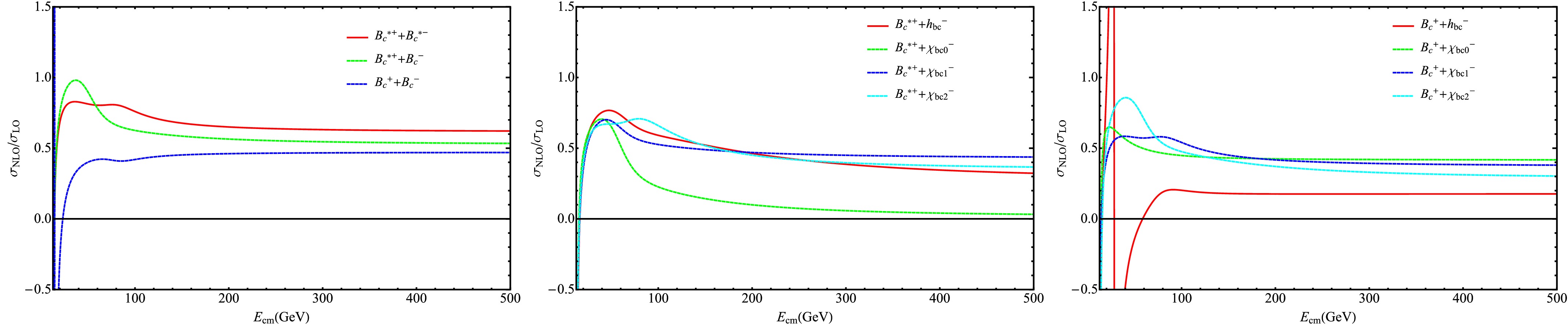

Figure 4.  (color online) $\sigma_{{\rm NLO}(v^2)}/\sigma_{\rm LO}$ versus c.m. energy. The left, middle, and right panels correspond to the production of double S-wave $ B_c $ meson, $ B_c^{*+}+X $, and $ B_c^++X $, respectively, where X denotes $ h_{bc}^- $ or $ \chi_{bcJ}^-(J=0,1,2) $.

The production of double charmonia or double bottomonia is governed by numerous conservation laws [16, 20]. For example, C-parity conservation forbids processes such as $ e^+e^- \to 2J/\psi, \; 2\eta_c, \; J/\psi+h_c, \; \eta_c+\chi_c $ from proceeding via a $ \gamma^* $ propagator. Furthermore, a given process proceeds exclusively via either the vector or the axial-vector part of the $ Z^0 $ current. For example, $ J/\psi+\eta_c $ production proceeds via the vector part, while $ \eta_c+\chi_c $ proceeds via the axial-vector part. For charged $ B_c $ mesons, these selection rules no longer hold. Consequently, we consider their P-parity properties. Weak interactions are known to violate P-parity; therefore, we define the P-asymmetry parameter $ {\cal{A}} $ following the definition in Ref. [69] as

For processes $ B_c^+ + B_c^- $ and $ B_c^+ + \chi_{bc0}^- $, this asymmetry is exactly zero at all energies because the axial-vector part of the $ Z^0 $ current ($ J^P=1^+ $) cannot produce two $ 0^- $ states, and the vector part ($ J^P=1^- $) cannot produce a $ 0^- + 0^+ $ state. Therefore, there is no V-A interference and no parity violation in these specific processes. For the same reason, the process $ B_c^+ + \chi_{bc0}^- $ ($ 0^-+0^+ $) cannot proceed via a γ-propagator ($ J^P=1^- $), as evident from Fig. 2. The asymmetry as a function of the collision energy is shown in Fig. 5. We find that the maximal asymmetry occurs at $ \sqrt{s} \simeq m_Z/2 $ and becomes nearly zero at the $ Z^0 $ resonance peak. Specifically, the asymmetry vanishes at the following energy points for different processes,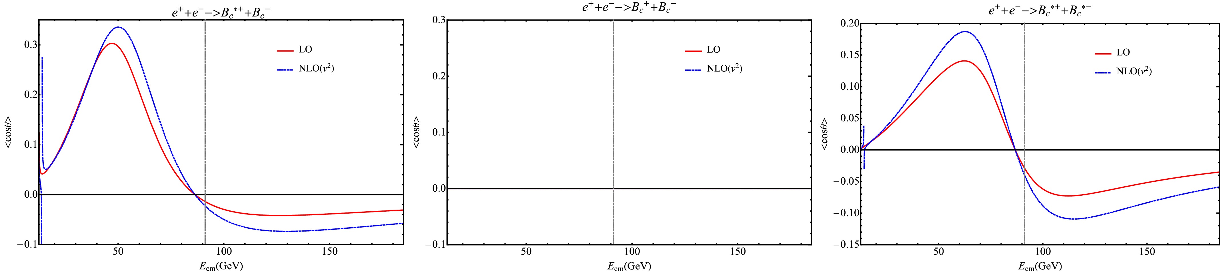

Figure 5.  (color online) Azimuthal asymmetry versus c.m. energy. The red solid and blue dashed lines represent the LO and NLO($ v^2 $) results, respectively. The vertical dashed line marks $ \sqrt{s}=m_Z $. The asymmetry is exactly zero for $ B_c^++B_c^- $ production.

Another notable feature is that the relativistic corrections slightly enhance the asymmetry. Moreover, we note that the azimuthal asymmetry $ \langle \cos\theta \rangle $ becomes nearly zero for all production processes at sufficiently high collision energies. For instance, in $ B_c^{*+} + \chi_{bcJ}^- $ production, this behavior occurs at $ \sqrt{s} \geqslant 1000\ \text{GeV} $. The angular distributions ${\rm d}\sigma/{\rm d}\cos\theta$ for three energy points ($ \sqrt{s} = m_Z/2,\ m_Z,\ 2m_Z $) are shown in Fig. 6, where θ is the angle between momenta of the electron ($ k_1 $) and the meson $ H_1 $ ($ p_1 $). The distributions are consistent with the azimuthal asymmetry results shown in Fig. 5. Specifically, the more symmetric the angular distribution, the closer the azimuthal asymmetry is to zero, and vice versa. Owing to the existence of the V-A interference term, the angular distributions of all processes except for $ B_c^++B_c^- $ and $ B_c^++\chi_{bc0}^- $ processes are asymmetric and correlate with the azimuthal asymmetry, and are generally described by a three-parameter functional form given by ${\rm d}\sigma/{\rm d} \cos\theta= A+B\cos\theta +C \cos^2\theta$. This form exhibits distinct behavior relative to that of double heavy quarkonium production in the s-channel, which obeys the trivial functional form given by ${\rm d}\sigma/{\rm d}\cos\theta=A(1+B \cos^2\theta)$[20, 103, 104]. ⁶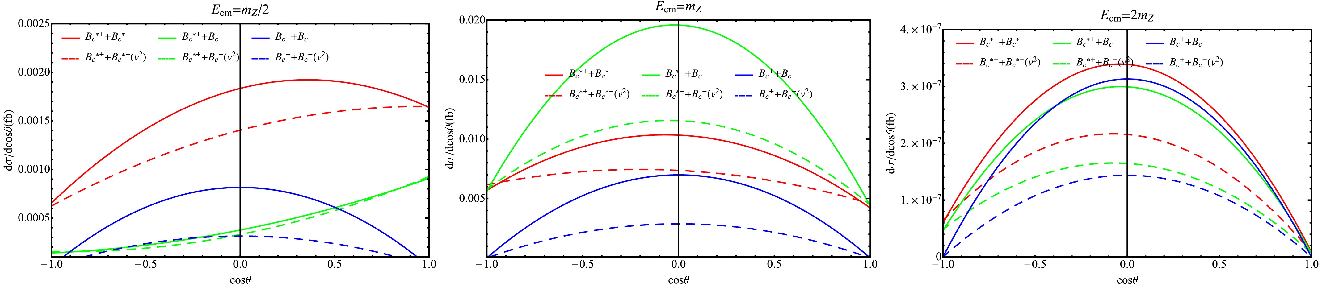

Figure 6.  (color online) Differential cross section ${\rm d}\sigma/{\rm d}\cos\theta$ at different c.m. energy. The left, middle and right panels correspond to $ \sqrt{s}=m_Z/2 $, $ \sqrt{s}=m_Z $, and $ \sqrt{s}=2m_Z $, respectively. The solid line represents LO results and the dashed line represents NLO($ v^2 $) results.

The transverse momentum distribution $\dfrac{{\rm d}\sigma}{{\rm d}p_t}$ can be written as

where the momentum of the $ H_1 $ meson is given by

Combining Eqs. (35) and (36), we can also get an $ {\cal{O}}(v^2) $ expression,

Using the above expressions, we show the transverse momentum distributions $ {\rm{d}}\sigma/{\rm{d}}p_t $ at different c.m. energy points in Fig. 7.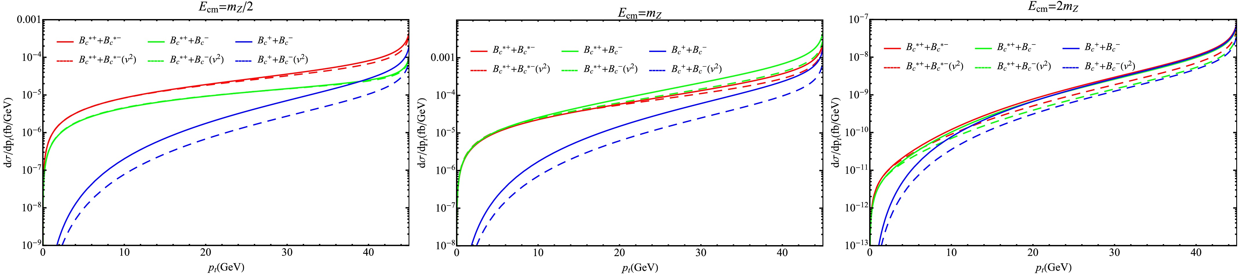

Figure 7.  (color online) Differential cross-section ${\rm d}\sigma/{\rm d}p_t$ at different c.m. energies. The left, middle, and right panels correspond to $ \sqrt{s}=m_Z/2 $, $ \sqrt{s}=m_Z $, and $ \sqrt{s}=2m_Z $, respectively. The solid and dashed lines represent the LO and NLO($ v^2 $) results, respectively.

CO contributions are significant in annihilation and hadron production processes [48, 105]; however, they are relatively small in electron-positron collisions [20, 31] and some indirect production mechanisms [56, 59]. The contributions of CO states are significant in the high energy region for double heavy quarkonium production in electron-positron collisions, where the gluon fragmentation process is most important [20]. In contrast, there are no gluon fragmentation diagrams for the production of paired $ B_c $ mesons.

The CO channels represent the inclusive processes for soft gluon emission or absorption. The complete calculations of LO inclusive production invoking ${\rm CS+ CO}+ g,\ {\rm CO+CO}+g$ are of the NLO of $ \alpha_s $ compared with the CS channels. For CO pair channels in a special case, in which the two final states with an energy close to half of the c.m. energy recoil without the emission of additional light particles, those contribute to the exclusive CS double mesons production in the experimental measurements. This specific configuration leads to the breakdown of factorization caused by nonperturbative effects, which are fortunately suppressed by the inverse powers of the collision energy and usually negligible. To obtain a rough estimate of these contributions, we follow the velocity scaling rules of NRQCD and the approach used in Refs. [31, 48, 56, 57, 59, 105], assuming a relationship between the CO and CS LDMEs.

Here, $ \Delta_S(v) $ is of order $ v^2 $, with typical values $ v^2 \sim 0.1 $–0.3, and $ \Delta_S(v) \sim \alpha_s(M_{B_c} v) $.

We now estimate the CO contribution to the cross-section at the $ Z^0 $ peak. As noted previously, the electroweak contributions are several orders of magnitude smaller than the QCD contributions, and therefore, it is sufficient to consider only $ \gamma/Z $–g type processes. The color factor for the CS amplitude squared is $ |C_s|^2 = C_F^2 $, while for the CO one it is $ |C_o|^2 = C_F/(2N_c) $. The CO cross-section is related to the CS cross-section as

Taking $ v^2 = 0.15 $ and considering $ B_c^{*+} + B_c^{-} $ production (via $ {}^3S_1^{[1]} + {}^1S_0^{[1]} $) as an example, the CS cross-section at the $ Z^0 $ peak is 0.030 fb. The four main CO channels are $ {}^3S_1^{[8]} + {}^1S_0^{[8]} $, $ {}^3S_1^{[8]} + {}^3S_1^{[8]} $, $ {}^1S_0^{[8]} + {}^3S_1^{[8]} $, and $ {}^1S_0^{[8]} + {}^1S_0^{[8]} $. The total CO cross section is then estimated as

This is approximately three orders of magnitude smaller than the CS contribution.

Theoretical uncertainties in our calculation arise from several sources, including the LDMEs, heavy quark masses, and the choice of renormalization scale.

For the LDMEs, various studies [51, 71, 83, 84, 97, 99] report values in the ranges $ |R_S(0)|^2 \in (1.30, 6.21) $ and $ |R'_P(0)|^2 \in (0.16, 0.90) $. Based on these ranges, we estimate that the LDMEs can introduce uncertainties of approximately –57% to +870% for double S-wave $ B_c $ production, and –66% to +809% for "S+P" waves $ B_c $ pair production.

The renormalization scale uncertainty is partially illustrated in Table 2. At $ \sqrt{s} = m_Z $, the dependence on the scale is similar to that observed in double heavy quarkonium production (cf. Figs. 10 and 11 in Ref. [20]): it decreases with increasing collision energy and leads to variations of ~–20% (for $ \mu=2m_Z $) to +128% (for $ \mu=2M_{B_c} $). For simplicity, these are not explicitly shown in the figures.

To quantify the uncertainties from the heavy quark masses, we adopt $ m_c = (1.5 \pm 0.3) $ GeV and $ m_b = (4.8 \pm 0.4) $ GeV, following Refs. [31, 58, 59]. The resulting total cross-sections at the $ Z^0 $ pole are presented in Tables 3 and 4. These cross-sections are more sensitive to the charm quark mass, consistent with the previous findings [31, 58, 59]. Further, we find that the cross-sections increase with decreasing charm quark mass; however, its decrease with decreasing bottom quark mass. This behavior is similar to that seen for the $ (c\bar{b})_1[{}^3S_1,{}^3P_2] $ states in Refs. [31, 59]. In general, the uncertainty caused by the $\pm0.3 \;{\rm GeV}$ variation of charm quark mass is –40%~+100% for double S-wave $ B_c $ meson production and –60%~+200% for P-wave $ B_c $ meson-involved production processes, whereas that caused by the $\pm0.4\;{\rm GeV}$ variation of bottom quark mass is –10%~+10% for double S-wave $ B_c $ meson production and –20%~+20% for P-wave $ B_c $ meson-involved production processes.

Based on the previous studies of $ B_c $ meson pair production in $ e^+e^- $ collisions, including LO calculation [17–19], NLO QCD correction [69], and relativistic corrections within the RQM to both s-channel [70] and t-channel double-photon processes [71], we investigated the relativistic corrections to double $ B_c $ production in $ e^+e^- $ annihilation within the NRQCD factorization framework [1], calculating both $ \gamma^* $- and $ Z^0 $-propagated processes, with c.m. energies ranging from the production threshold $ 2M_{B_c} $ up to $ 2m_Z $.

The results confirm that the relativistic corrections are substantial, with K-factors of ~0.6, which correspond to a 40% reduction of the LO cross-sections. This effect is comparable in magnitude to the NLO QCD corrections, which have K-factors of ~1.4 [69]. Further, we present the azimuthal asymmetry arising from P-parity violation as a function of the c.m. energy, along with the differential cross-sections (angular distribution and transverse momentum distribution) at specific energy points ($ m_Z/2 $, $ m_Z $, and $ 2m_Z $). In addition, the theoretical uncertainties from quark masses and renormalization scale are discussed.

Considering the negligible contributions from the t-channel double-photon mechanism and CO states, the small reconstruction efficiency or decay branching fractions (e.g., $ {\cal{B}}(B_c^{\pm} \to J/\psi \pi^{\pm}) $≈0.5% [106]), and the significant negative relativistic corrections, the observation of double $ B_c $ production remains challenging (as also pointed out in Ref. [67]) for future $ ee $ collider Z-factory experiments despite the enhancing effect of NLO QCD corrections [69].

Therefore, alternative production modes may be more promising. These include operation near the production threshold ($\sqrt{s} \sim 15\ {\rm{GeV}}$, a ''$ \ B_c^* $-factory'' [69]), or hadronic [41, 50, 51, 76] and photonic [41, 43, 44] production mechanisms. Finally, beyond QCD corrections for $ B_c $-related processes, further calculation of relativistic corrections, which are relatively less studied, will be essential for gaining a deeper understanding of QCD and the properties of $ B_c $ mesons.

We present the short-distance coefficient (SDC) ratios of the relativistic corrections (denoted as G) relative to the LO ones (denoted as F) for the processes $ e^+e^-\rightarrow Z^0/\gamma^*\rightarrow (c\bar{b}) [{}^{2S_1+1}{L_1}_{J_1}]+(b\bar{c})[{}^{2S_2+1}{L_2}_{J_2}] $ in the high-collision energy limit ($ M^2\ll s $). Further, we define $ R_i=G[n_i]/F[n_1+n_2] $ (where $ n_i,i=1,2 $ represent the final Fock states) and $ \xi=m_c/m_b $ in the following expressions. For the production of double S-wave states, we present the analytical expressions for different propagation processes: γ-propagator, $ Z^0 $-propagator, and the sum of the two processes including interference effects.

For $ { }^3S_1^{[1]}+{ }^1S_0^{[1]} $ production, the $ Z^0 $-propagated process cross-section ratios are

The $ \gamma^* $-propagated process cross-section ratios are

The total cross-section ratios are identical to those of the $ Z^0 $-propagated process Eqs. (A1) and (A2) because this process dominates overwhelmingly at high collision energies, and as shown in the first panel of Fig. 2, it is orders of magnitude larger than the $ \gamma^* $-propagated process in the cross-section.

For $ { }^3S_1^{[1]}+{ }^3S_1^{[1]} $ production, $ Z^0 $-propagated process cross section ratios,

The $ \gamma^* $-propagated process cross-section ratios are

The total cross-section ratios are

For $ { }^1S_0^{[1]}+{ }^1S_0^{[1]} $ production, $ Z^0 $-propagated process cross section ratios,

The $ \gamma^* $-propagated process cross-section ratios are

The total cross-section ratios are

When $ m_c=m_b $ (i.e. $ \xi=1 $), these ratios are consistent with that in Refs. [20, 92–94].

For simplicity, we only show the numerical values of ratios R for other processes in Table A1.