


 Abstract
 HTML
HTML Reference
 Related
 PDF
PDF


-
The study of non-
$ q\bar{q} $ mesons beyond the conventional quark model remains a central topic in hadron physics [1, 2]. QCD predicts the existence of mesons with various structures, such as hybrid states containing excited gluons [3, 4], glueballs composed purely of gluons [5], and multiquark states [6–11]. Mesons with the exotic quantum numbers$ J^{PC}=1^{-+} $ have attracted much attention and are typically regarded as candidates for hybrids, tetraquarks, or their mixtures. In particular, the ambiguity surrounding the isovector state$ \pi_1(1400) $ has persisted for a long time.$ \pi_1(1400) $ appeared in the$ \pi^- p \to \pi^0 \eta n $ reaction [12], and it was later observed in the$ \pi^- p \to \eta \pi^- p $ channel [13, 14]. However, some recent evidence suggests that$ \pi_{1}(1400) $ may be an artifact of the$ \pi_{1}(1600) $ particle and might not exist [15]. Based on the partial-wave analysis data of the$ \eta^{(\prime)}\pi $ system provided by the COMPASS Collaboration [16], Ref. [17] performs a coupled-channel amplitude analysis that enforces the unitarity and analyticity of the S matrix, demonstrating that a single pole is sufficient to fit the experimental data for both$ \pi_1(1400) $ and$ \pi_1(1600) $ . In Ref. [18],$ \pi_{1}(1400) $ was interpreted as a molecular tetraquark, while Ref. [19] suggested that a hybrid-tetraquark mixture might explain$ \pi_{1}(1400) $ , a conclusion also reached in later work [20]. Studies on hybrids indicate that the mass of a$ 1^{-+} $ hybrid state is higher than$ 1.7\,\text{GeV} $ [21–23], making it difficult to match the mass of$ \pi_{1}(1400) $ . Therefore, within the framework of QCD sum rules, the existence of$ \pi_{1}(1400) $ depends on whether there exists a tetraquark state with a mass close to or less than$ 1.4\,\text{GeV} $ . In Ref. [24], a series of compact tetraquark currents were calculated, and several isospin-1$ 1^{-+} $ compact tetraquark states with masses around$ 1.6\,\text{GeV} $ and$ 2.0\,\text{GeV} $ were obtained. Therefore,$ \pi_{1}(1600) $ and$ \pi_{1}(2015) $ are regarded as suitable candidates for four-quark states. However, all the studies mentioned above on tetraquark states were calculated only at leading order (LO) without considering next-to-leading-order (NLO) contributions, which can sometimes be significant [3]. In this work, we present the first NLO analysis of the$ 1^{-+} $ tetraquark states. Using the latest phenomenological parameters and a more precise running coupling, we reanalyze the possibility of the existence of$ \pi_1(1400) $ , and examine whether$ \pi_1(1600) $ and$ \pi_1(2015) $ can be suitable tetraquark candidates. -
Previous studies showed that some currents with u, d, and s quarks (and their antiquarks) give
$ 1^{-+} $ states with masses around$ 1.4 $ –$ 2.0\,\text{GeV} $ at leading order. [18, 24]. We expect that adding NLO corrections should shift their masses. This makes them a good choice for our study. We built the compact tetraquark currents using quark pairs ($ qq $ ) and antiquark pairs ($ \bar{q}\bar{q} $ ). Based on charge conjugation and flavor structure, we defined four currents$ \eta_{1}^{\mu} \sim \eta_{4}^{\mu} $ :$ \begin{aligned}[b] \eta_1^\mu=\;&u_a^T C\gamma^\mu d_b (\bar{u}_aC\bar{d}^{\,T}_b + \bar{u}_bC\bar{d}^{\,T}_a) \\&+ u_a^T C d_b (\bar{u}_a\gamma^\mu C\bar{d}^{\,T}_b + \bar{u}_b\gamma^\mu C\bar{d}^{\,T}_a),\\ \eta_2^\mu=\;&u_a^T C\sigma^{\mu\nu}\gamma^5 d_b (\bar{u}_a\gamma_\nu\gamma^5C\bar{d}^{\,T}_b + \bar{u}_b\gamma_\nu\gamma^5C\bar{d}^{\,T}_a) \\&+ u_a^T C \gamma_\nu\gamma^5d_b (\bar{u}_a\sigma^{\mu\nu}\gamma^5C\bar{d}^{\,T}_b + \bar{u}_b\sigma^{\mu\nu}\gamma^5 C\bar{d}^{\,T}_a),\\ \eta_3^\mu=\;&u_a^T C\gamma^\mu d_b (\bar{u}_aC\bar{d}^{\,T}_b - \bar{u}_bC\bar{d}^{\,T}_a)\\& + u_a^T C d_b (\bar{u}_a\gamma^\mu C\bar{d}^{\,T}_b - \bar{u}_b\gamma^\mu C\bar{d}^{\,T}_a),\\ \eta_4^\mu=\;&u_a^T C\sigma^{\mu\nu}\gamma^5 d_b (\bar{u}_a\gamma_\nu\gamma^5C\bar{d}^{\,T}_b - \bar{u}_b\gamma_\nu\gamma^5C\bar{d}^{\,T}_a) \\&+ u_a^T C \gamma_\nu\gamma^5d_b (\bar{u}_a\sigma^{\mu\nu}\gamma^5C\bar{d}^{\,T}_b - \bar{u}_b\sigma^{\mu\nu}\gamma^5 C\bar{d}^{\,T}_a),\\ \end{aligned} $
(1) where C is the charge conjugation operator, and
$ \sigma^{\mu\nu} = \frac{i}{2} [\gamma^{\mu}, \gamma^{\nu}] $ . Replacing the d quark with an s quark, we obtain$ \begin{aligned}[b] \eta_5^\mu=\;&u_a^T C\gamma^\mu s_b (\bar{u}_aC\bar{s}^T_b + \bar{u}_bC\bar{s}^T_a) \\&+ u_a^T C s_b (\bar{u}_a\gamma^\mu C\bar{s}^T_b + \bar{u}_b\gamma^\mu C\bar{s}^T_a),\\ \eta_6^\mu=\;&u_a^T C\sigma^{\mu\nu}\gamma^5 s_b (\bar{u}_a\gamma_\nu\gamma^5C\bar{s}^T_b + \bar{u}_b\gamma_\nu\gamma^5C\bar{s}^T_a)\\& + u_a^T C \gamma_\nu\gamma^5s_b (\bar{u}_a\sigma^{\mu\nu}\gamma^5C\bar{s}^T_b + \bar{u}_b\sigma^{\mu\nu}\gamma^5 C\bar{s}^T_a),\\ \eta_7^\mu=\;&u_a^T C\gamma^\mu s_b (\bar{u}_aC\bar{s}^T_b - \bar{u}_bC\bar{s}^T_a) \\&+ u_a^T C s_b (\bar{u}_a\gamma^\mu C\bar{s}^T_b - \bar{u}_b\gamma^\mu C\bar{s}^T_a),\\ \eta_8^\mu=\;&u_a^T C\sigma^{\mu\nu}\gamma^5 s_b (\bar{u}_a\gamma_\nu\gamma^5C\bar{s}^T_b - \bar{u}_b\gamma_\nu\gamma^5C\bar{s}^T_a) \\&+ u_a^T C \gamma_\nu\gamma^5s_b (\bar{u}_a\sigma^{\mu\nu}\gamma^5C\bar{s}^T_b - \bar{u}_b\sigma^{\mu\nu}\gamma^5 C\bar{s}^T_a). \end{aligned} $
(2) Furthermore, for molecular tetraquark states, we also consider the following two currents [18]
$ J_1^\mu =\frac{1}{2}\left(\bar{u}\gamma^5 u-\bar{d}\gamma^5d\right)\left(\bar{u}\gamma^5\gamma^\mu u+\bar{d}\gamma^5\gamma^\mu d\right), $
(3) $ J_2^{\mu\nu} =\epsilon^{\mu\nu\rho\sigma}\left(\bar{u}\gamma^5\gamma_\rho d \,\bar{d}\gamma_\sigma u - \bar{d}\gamma^5\gamma_\rho u \,\bar{u}\gamma_\sigma d\right), $
(4) where
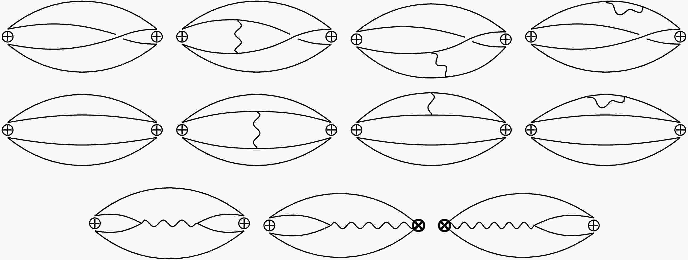
$ \epsilon^{\mu\nu\rho\sigma} $ is the totally antisymmetric tensor, with the convention$ \epsilon^{0123}=+1 $ .When expanding the perturbative part of the correlation functions for these tetraquark currents to NLO, we need to calculate the Feynman diagrams as shown in Fig. 1. Since tetraquark currents are composite operators, the calculation results will contain non-local divergence terms such as
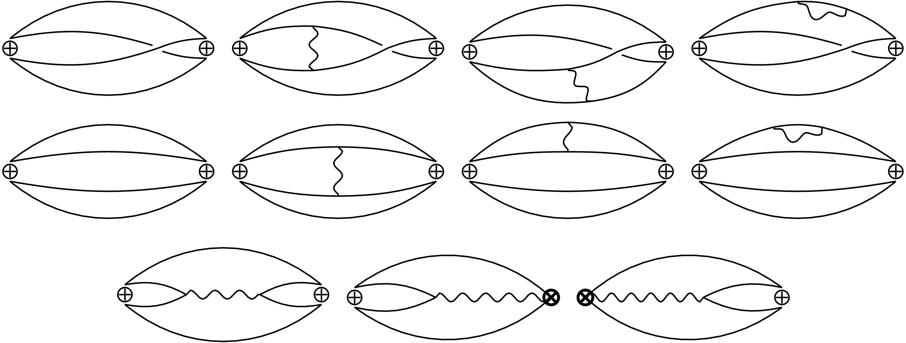
Figure 1. Feynman diagrams for the perturbative term of tetraquark currents. Permutation diagrams are omitted. The bold cross vertex represents the hybrid-like counterterm. For compact tetraquark currents, the first four diagrams are unnecessary.
$ \log(-q^2/\mu^2)/\varepsilon. $
(5) These non-local divergences cannot be completely removed by conventional Lagrangian renormalization methods; the operator currents themselves must be renormalized. For operator currents
$ \eta_1^\mu $ and$ \eta_3^\mu $ , using the tetraquark renormalization method in Ref. [25], with the Feynman gauge, we can obtain$ \begin{aligned}[b] &\left(u_a^T C d_b \,\bar{u}_a\gamma^\mu C\bar{d}^{\,T}_b\right)_r\\=\;&\left(Z_2^{-2}-\frac{2C_A^2+1 }{32\pi^2\varepsilon C_A}g^2\right)u_a^T C d_b\,\bar{u}_a\gamma^\mu C\bar{d}^{\,T}_b \\&+ \frac{3}{32\pi^2\varepsilon}g^2u_a^T C d_b\,\bar{u}_b\gamma^\mu C\bar{d}^{\,T}_a\\ &-\frac{C_A i g^2}{32\pi^2\varepsilon}u_a^T C\sigma^{\mu\nu}\gamma^5 d_b \,\bar{u}_a\gamma_\nu\gamma^5C\bar{d}^{\,T}_b \\&+ \frac{i g^2}{32\pi^2\varepsilon}u_a^T C\sigma^{\mu\nu}\gamma^5 d_b \,\bar{u}_b\gamma_\nu\gamma^5C\bar{d}^{\,T}_a , \end{aligned} $
(6) $ \begin{aligned}[b] &\left(u_a^T C d_b \,\bar{u}_b\gamma^\mu C\bar{d}^{\,T}_a\right)_r\\=\;&\left(Z_2^{-2}-\frac{2C_A^2+1 }{32\pi^2\varepsilon C_A}g^2\right)u_a^T C d_b\,\bar{u}_b\gamma^\mu C\bar{d}^{\,T}_a \\&+ \frac{3}{32\pi^2\varepsilon}g^2u_a^T C d_b\,\bar{u}_a\gamma^\mu C\bar{d}^{\,T}_b\\ &+\frac{C_A i g^2}{32\pi^2\varepsilon}u_a^T C\sigma^{\mu\nu}\gamma^5 d_b \,\bar{u}_b\gamma_\nu\gamma^5C\bar{d}^{\,T}_a \\&- \frac{i g^2}{32\pi^2\varepsilon}u_a^T C\sigma^{\mu\nu}\gamma^5 d_b \,\bar{u}_a\gamma_\nu\gamma^5C\bar{d}^{\,T}_b\\ &+\frac{1}{48\pi^2\varepsilon}\left(\bar{u}D^\alpha G_{\alpha\beta} \gamma^\beta\gamma^\mu\gamma^5 u - \bar{d}D^\alpha G_{\alpha\beta} \gamma^\beta\gamma^\mu\gamma^5 d\right) , \end{aligned} $
(7) In the above equations,
$ Z_2=1-\frac{g^2 C_F}{16\pi^2\epsilon}, $
(8) where
$ C_F=4/3 $ is the quadratic Casimir operator of the fundamental representation of the$ SU(3) $ group, and$ C_A=3 $ is the quadratic Casimir operator of the adjoint representation of the$ SU(3) $ group; these parameters are also known as the quark and gluon color factors, respectively. For convenience, we suppress the generator matrix T of$ SU(3) $ and the coupling constant g, i.e.,$ D^\alpha G_{\alpha\beta} \equiv g D^\alpha G^n_{\alpha\beta} T^n. $
(9) The hybrid-like current
$ D^\alpha G_{\alpha\beta} $ only appears in operator currents where the summation is over different quark color indices. By replacing the d quark in Eqs. (6) and (7) with an s quark, we obtain the operator renormalization results for tetraquark currents$ \eta_5^\mu $ and$ \eta_7^\mu $ . As for the molecular tetraquark currents, they can be obtained through linear combinations of the following renormalized operator currents:$\begin{aligned}[b] \left(\bar{u}\gamma^5 u\,\bar{d}\gamma^5\gamma^\mu d\right)_r=\;& \left(Z_2^{-2}+\frac{5C_F}{16\pi^2\varepsilon}g^2\right)\bar{u}\gamma^5 u\,\bar{d}\gamma^5\gamma^\mu d \\&+ \frac{ig^2}{8\pi^2\varepsilon}\bar{u}T^n\sigma^{\mu\nu}u\,\bar{d}\gamma_\nu T^n d,\end{aligned} $
(10) $ \begin{aligned}[b] \left(\bar{u}\gamma^5 u\,\bar{u}\gamma^5\gamma^\mu u\right)_r=\;&\left(Z_2^{-2}+\frac{5C_F}{16\pi^2\varepsilon}g^2\right)\bar{u}\gamma^5 u\,\bar{u}\gamma^5\gamma^\mu u \\&+ \frac{ig^2}{8\pi^2\varepsilon}\bar{u}T^n\sigma^{\mu\nu}u\,\bar{u}\gamma_\nu T^n u\\ &+\frac{i}{24\pi^2\varepsilon}\bar{u}D^\alpha G_{\alpha\beta}\sigma^{\beta\mu}u. \end{aligned} $
(11) The renormalization of other operator currents is placed in Appendix A.2.
-
QCD sum rules [2, 26–29] determine the corresponding hadronic spectral structure through the poles of operator current correlation functions in the complex plane. To calculate the correlation function, we first perform an Operator Product Expansion (OPE):
$\begin{aligned}[b] \Pi(q)=\;&i\int d^4x e^{iqx}\langle 0|T\{J^\mu(x) J^\nu(0)\}|0\rangle \\=\;& C_0(q) + C_4(q)\langle O^4\rangle + C_6(q)\langle O^6\rangle +\cdots,\end{aligned} $
(12) where
$ C_i(q) $ are Wilson coefficients, and$ \langle O^i\rangle $ denote vacuum condensates (i.e., the vacuum expectation values of various local operators). The first Wilson coefficient$ C_0(q) $ corresponds to the perturbative diagrams in Fig. 1, which accounts for the high-energy contribution. Subsequent coefficients like$ C_4(q) $ and$ C_6(q) $ can be calculated by cutting certain propagators in the perturbative diagrams or introducing zero-momentum gluons from the vacuum; they represent the contribution from the low-energy region. For this part of the contribution, it is suitable to calculate in coordinate space. We can use the techniques in Refs. [24, 30–32] to handle these non-perturbative contributions. The quark propagator including vacuum condensates is$ \begin{align} i S^{ab} &\equiv \langle 0 | T [ q^a(x) \bar{q}^b(0) ] | 0 \rangle\\ &= { i \delta^{ab} \over 2 \pi^2 x^4 } \not{x} - {ig \over 32\pi^2} G^n_{\mu\nu} T^{n\,ab}{1 \over x^2} (\sigma^{\mu\nu}\not{x} + \not{x}\sigma^{\mu\nu}) - { \delta^{ab} \over 12 } \langle \bar q q \rangle \\ &\quad - { \delta^{ab} x^2 \over 192 } \langle g \bar q \sigma G q \rangle - { m_q \delta^{ab} \over 4 \pi^2 x^2 } + { i \delta^{ab} m_q \langle \bar q q \rangle \over 48 } \not{x} + { i \delta^{ab} m_q^2 \over 8 \pi^2 x^2 } \not{x} \end{align} $
(13) The Lorentz structure of operator currents indicates that a general vector current can couple to both vector particles and scalar particles. Therefore, we need to isolate the part corresponding to the
$ 1^{-+} $ vector particle in the correlation function. In momentum space, the correlation function of the vector current can be decomposed into$\begin{aligned}[b]& i\int d^4x e^{iqx}\langle 0|T\{J^\mu(x) J^\nu(0)\}|0\rangle \\=\;& \left(\frac{q^\mu q^\nu}{q^2}-g^{\mu\nu}\right)\Pi^V(q) + q^\mu q^\nu\Pi^S(q),\end{aligned} $
(14) where the term
$ \left(\dfrac{q^\mu q^\nu}{q^2}-g^{\mu\nu}\right) $ on the right side of the equation is the transverse polarization factor, and$ q^\mu q^\nu $ is the longitudinal polarization factor. The vector particle couples to the vector current$ J^\mu $ through the matrix element$ \langle 0|J^\mu|V(q)\rangle=\epsilon^\mu f(q^2). $
(15) Meanwhile, the polarization vector
$ \epsilon^\mu $ satisfies the completeness relation$ \sum\limits_{\lambda=-1}^{1}\epsilon_{\lambda}^{\mu*}\,\epsilon_{\lambda}^{\nu}=\frac{q^\mu q^\nu}{q^2}-g^{\mu\nu}. $
(16) Therefore, the spectral density of the vector particle is related to the transverse polarization part of the correlation function. For vector currents
$ \eta_1^\mu \sim \eta_8^\mu $ and$ J_1^\mu $ , only the$ \Pi^V(q) $ part is considered. For tensor currents, they can couple to scalar particles, vector particles, and tensor particles. Similar to the analysis above, considering that$ J_2^{\mu\nu} $ is antisymmetric with respect to Lorentz indices, we decompose the tensor current operator correlation function in momentum space as$ \begin{aligned}[b] & i\int d^4x e^{iqx}\langle 0|J_2^{\mu\nu}(x)\, J_2^{\dagger\,\alpha\beta}|0\rangle=(\eta^{\mu\alpha}\eta^{\nu\beta}-\eta^{\nu\alpha}\eta^{\mu\beta})\Pi_{J_2}^{\prime V}(q^2)\\ &\quad+(\eta^{\mu\alpha}q^\nu q^\beta - \eta^{\nu\alpha}q^\mu q^\beta - \eta^{\mu\beta}q^\nu q^\alpha + \eta^{\nu\beta}q^\mu q^\alpha)\frac{1}{q^2}\Pi_{J_2}^V(q^2), \end{aligned} $
(17) where
$ \eta^{\mu\nu}\equiv\dfrac{q^\mu q^\nu}{q^2}-g^{\mu\nu} $ . The coupling rule for vector particles and tensor currents is$ \langle 0|J_2^{\mu\nu}|V(q)\rangle=(q^\mu\epsilon^\nu - q^\nu\epsilon^\mu) f(q^2). $
(18) Combined with Eq. (16), it can be seen that the spectral density of the vector particle corresponds to the
$ \Pi_{J_2}^V(q^2) $ part.We derive the OPE of the correlation function using dimensional regularization and the
$ \overline{\text{MS}} $ subtraction scheme, while treating$ \gamma^5 $ in the BMHV scheme. Consequently, the correlation function$ \Pi^V $ for the current$ \eta_1^\mu $ is given by$ \begin{aligned}[b] \Pi^V_{\eta_1}=\;&q^8\Bigg[ \left(-\frac{79 g_s^2}{2654208 \pi ^8}-\frac{1}{18432 \pi ^6}\right) \log \left(-\frac{q^2}{\mu ^2}\right)\\&-\frac{5 g_s^2 }{1327104 \pi ^8}\log ^2\left(-\frac{q^2}{\mu ^2}\right)\Bigg] \\ &+q^4\frac{ g_s^2 }{18432 \pi ^6}\log \left(-\frac{q^2}{\mu ^2}\right) \langle GG \rangle\\&-q^2\frac{ 1}{18 \pi ^2}\log \left(-\frac{q^2}{\mu ^2}\right) \langle \bar{q}q \rangle ^2\\ &+\frac{1}{12 \pi ^2}\log \left(-\frac{q^2}{\mu ^2}\right) \langle \bar{q}q \rangle \langle \bar{q}Gq \rangle \\&+\frac{1}{q^2}\left(\frac{5 g_s^2 }{864 \pi ^2}\langle GG \rangle \langle \bar{q}q \rangle ^2-\frac{1}{48 \pi ^2}\langle \bar{q}Gq \rangle ^2\right)\\ &+\frac{1}{q^4}\left(-\frac{g_s^2}{576 \pi ^2} \langle GG \rangle \langle \bar{q}q \rangle \langle \bar{q}Gq \rangle -\frac{32}{81} g_s^2 \langle \bar{q}q \rangle ^4\right). \end{aligned} $
(19) The remaining correlation functions are given in Appendix A.3.
Using the dispersion relation and adopting the "δ + continuum" assumption, we have
$ \frac{1}{\pi}\text{Im}\Pi^V(q) = f^2\delta(s-m^2)+\theta(s-s_0)\rho_c(s), $
(20) where m is the mass of the lowest resonance state, f is the coupling strength,
$ s_0 $ is the continuum threshold, and$ \rho_c(s) $ is the spectral density of the continuum states. Applying the Borel transform to both sides of the above equation yields the n-th moment$ {\cal{M}}^n(\tau,s_0) $ :$ {\cal{M}}^n(\tau,s_0)\equiv\frac{1}{\pi}\int_0^{s_0}ds\ s^n e^{-\tau s}\, \text{Im}\Pi^V(s)=f^2 m^{2n}e^{-\tau m^2}. $
(21) The mass m of the lowest resonance state in the spectral density can be obtained from the ratio of the moment:
$ {\cal{R}}^n(\tau,s_0)\equiv\frac{{\cal{M}}^{n+1}(\tau,s_0)}{{\cal{M}}^n(\tau,s_0)}=m^2, $
(22) By taking the ratio of moments, the coupling constant f cancels out. In this paper, we take
$ n=0 $ . -
In the numerical analysis, we adopt the following quark masses and vacuum condensate parameters at the scale
$ \mu = 2\,\text{GeV} $ [33, 34]:$ \begin{align*} m_s &= 93.5\pm 0.8\,\text{MeV},\\ \frac{g^2}{4\pi}\langle GG\rangle & = 0.07\pm0.02\,\text{GeV}^4,\\ \langle \bar{q}q\rangle &= -(0.276)^3\,\text{GeV}^3,\\ \langle\bar{s}s\rangle &= 0.74\langle \bar{q}q\rangle,\\ \langle\bar{q}Gq\rangle &= M_0^2\langle \bar{q}q\rangle,\\ \langle\bar{s}Gs\rangle &= M_0^2\langle \bar{s}s\rangle,\\ M_0^2&=0.8\pm0.2\,\text{GeV}^2, \end{align*} $
where
$ q=u \text{ or } d $ ,$ \langle GG\rangle = \langle G^n_{\mu\nu}G^{n\mu\nu}\rangle $ ,$ \langle \bar{q}Gq\rangle= \langle\bar{q}gT^nG^n_{\mu\nu}\sigma^{\mu\nu}q\rangle $ , and the masses of light quarks u and d are neglected. The running coupling constant$ \alpha_s $ is taken in the one-loop approximation:$ \alpha_s(\mu^2)=\frac{\alpha_s(m^2_\tau)}{1+\dfrac{\beta_0}{4\pi}\alpha_s(m^2_\tau)\log\big(\dfrac{\mu^2}{m^2_\tau}\big)}, $
(23) where
$ m_\tau=1776.93\pm0.09\,\text{MeV} $ ,$ \alpha_s(m^2_\tau)=0.314\pm0.014 $ , with$ n_f=3 $ and$ \beta_0=9 $ . Renormalization-group improvement is achieved by setting$ \mu^2=1/\tau $ [35].We calculated the relative contributions of the perturbative term and condensate terms to the moment
$ {\cal{M}}^0(\tau,s_0) $ of the current$ \eta_1^{\mu} $ , as shown in Fig. 2. It can be seen that the OPE converges well, so the calculation results are reliable.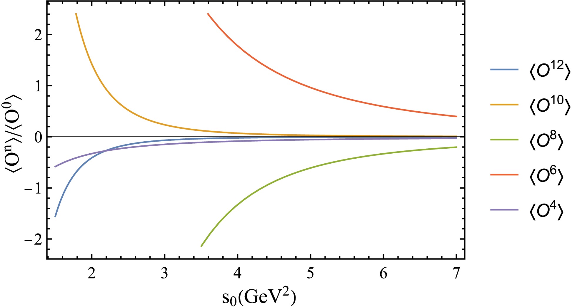
Figure 2. (color online) Ratio of condensate terms
$ \langle O^n\rangle $ to the perturbative term$ \langle O^0\rangle $ for$ \eta_1^{\mu} $ , at$ \tau=0.3\; {\rm{GeV}}^{-2} $ .Using the ratio of moments in Eq. (22), we extract the mass of the lowest resonance by
$ m=\sqrt{{\cal{R}}^0(\tau,s_0)} $ , which depends on the Borel parameter τ and the continuum threshold$ s_0 $ . Since the Borel parameter τ is auxiliary, the extracted mass should exhibit a stable plateau with respect to τ. We determine the mass using stability criteria [34]: the mass is extracted from the extremum of the$ m(\tau) $ curve or its plateau region1 . The general procedure is to first determine an approximate value of$ s_0 $ such that a plateau appears in the$ m(\tau) $ curve. Subsequently, the range of τ corresponding to this plateau is identified as the working region. Finally, the mass of the resonance state is determined by the value of m at the plateau. It is worth noting that the moment$ {\cal{M}}^0 $ corresponds to the spectral density and thus is always positive. If a negative value appears, it indicates that the QCD sum rules analysis breaks down, and the corresponding mass is non-physical. In Fig. 3, we list the$ {\cal{M}}^0 \sim s_0 $ and$ m \sim s_0 $ curves for the tensor current$ J_2^{\mu\nu} $ . In the left figure, the region$ s_0\lesssim 4.5\,\text{GeV}^2 $ is non-physical, so the corresponding mass$ \lesssim 1.5\,\text{GeV} $ in the right figure is not credible; the true mass should be$ \gtrsim2.3\,\text{GeV} $ . In the subsequent analysis, we discuss within the physical interval where$ {\cal{M}}^0 $ is positive.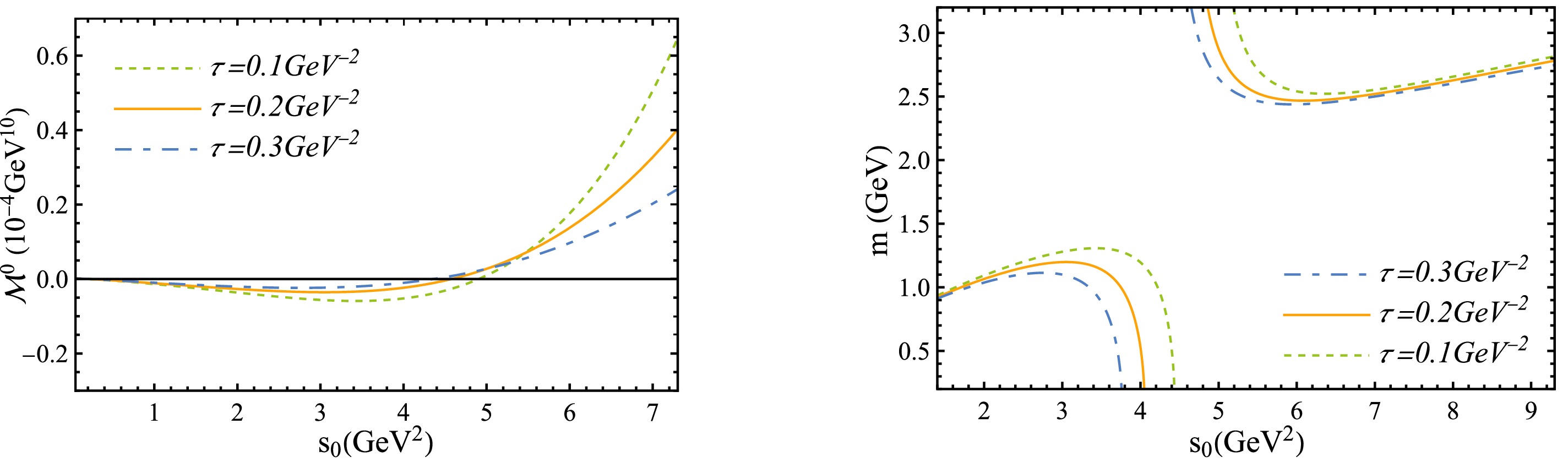
Figure 3. (color online) NLO results for the moment
$ {\cal{M}}^0 $ and mass m versus the$ s_0 $ for the current$ J_2^{\mu\nu} $ Fig. 4 shows that, for
$ J^{\mu\nu}_2 $ , the NLO perturbative correction is roughly 30% of the LO contribution and thus cannot be neglected. For$ \eta^\mu_2 $ , the NLO perturbative correction is even larger than the LO term, reaching about 130% of the LO contribution. Furthermore, in Fig. 5, the left side shows the estimated mass of the operator current$ J^{\mu\nu}_2 $ when expanded to LO, and the right side shows the estimated mass after adding the NLO perturbation correction. Including the NLO correction significantly affects the mass determination. In particular, the mass curve is lowered by roughly$ 0.2\,\text{GeV} $ and becomes flatter, which leads to improved stability.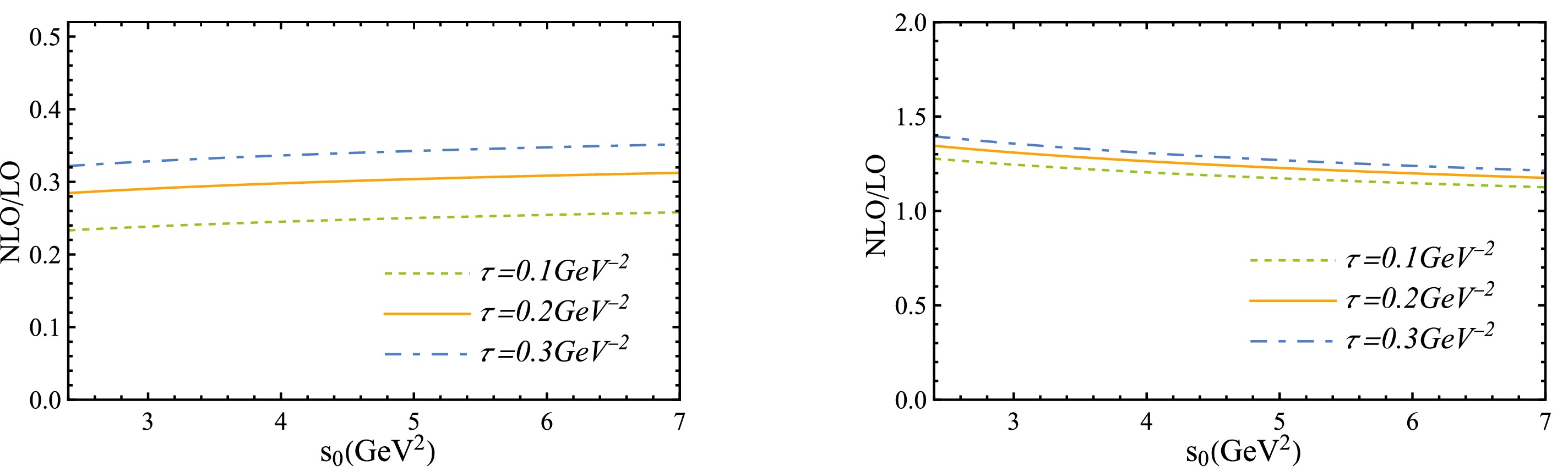
Figure 4. (color online) Ratio of NLO contribution to LO contribution in moment
$ {\cal{M}}^0 $ for the currents$ J_2^{\mu\nu} $ (left) and$ \eta_2^\mu $ (right).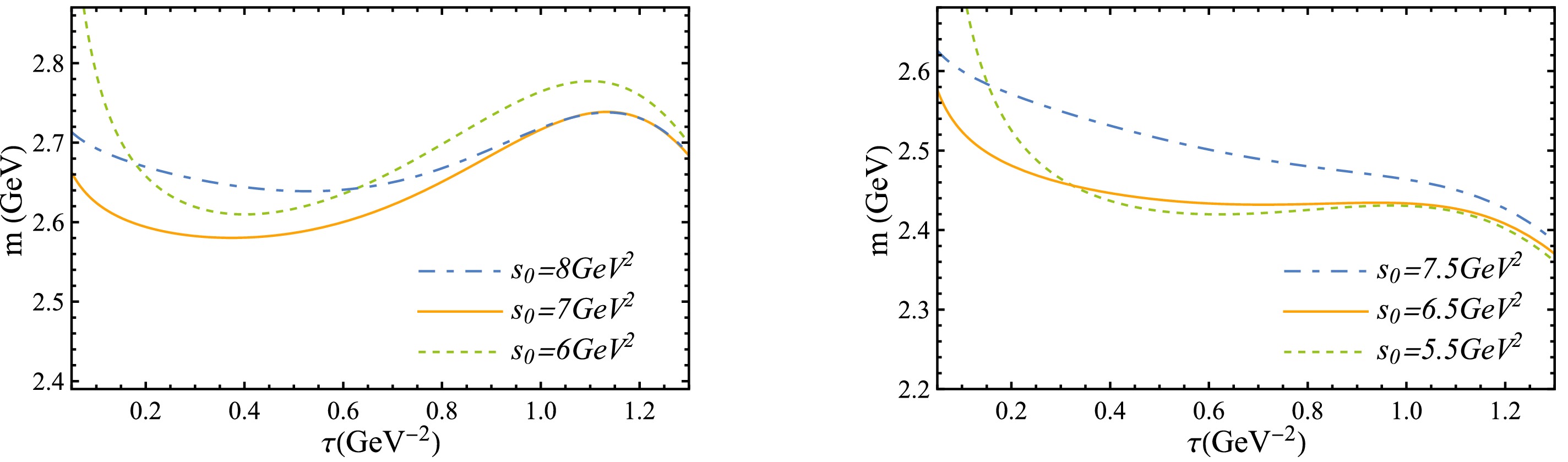
Figure 5. (color online) Mass predictions for the current
$ J_2^{\mu\nu} $ at LO (left) and NLO (right) levels.In Appendix A.1, we present the curves of the resonance mass m as a function of the Borel parameter τ for all currents, with
$ s_0 $ fixed at various values. Based on the stability criterion, we select three$ s_0 $ values that yield the flattest curves in each figure. The corresponding optimal mass estimates and$ s_0 $ values are listed in Table 1. The masses for the compact tetraquark currents$ \eta_1^\mu \sim \eta_4^\mu $ (with u and d quarks) are$ 2.05\,\text{GeV} $ ,$ 1.88\,\text{GeV} $ ,$ 1.70\,\text{GeV} $ , and$ 1.99\,\text{GeV} $ . For$ \eta_5^\mu\sim\eta_8^\mu $ (with u and s quarks), the corresponding masses are$ 2.36\,\text{GeV} $ ,$ 2.06\,\text{GeV} $ ,$ 2.26\,\text{GeV} $ , and$ 2.34\,\text{GeV} $ . For the molecular currents, we obtain$ 1.71\,\text{GeV} $ for$ J_1^\mu $ and$ 2.44\,\text{GeV} $ for$ J_2^{\mu\nu} $ . In previous LO studies [24], the currents$ \eta_1^\mu \sim \eta_4^\mu $ yield lowest resonance masses around$ 1.6 $ –$ 1.7\,\text{GeV} $ and are considered to couple to the$ \pi_1(1600) $ . However, after NLO corrections, the lowest resonance masses increase, moving away from the peak position of the$ \pi_1(1600) $ . In comparison with previous LO QCD sum rules studies, our mass predictions are shifted by$ 0.1 \sim 0.3\,\text{GeV} $ for each current, as shown in Appendix A.4. These corrections are primarily attributed to the NLO contributions, as well as the updated QCD parameters, the use of a more precise running coupling, and renormalization group improvements.$ \eta_1 $ $ \eta_2 $ $ \eta_3 $ $ \eta_4 $ $ \eta_5 $ m $ 2.05\pm0.05 $ $ 1.88\pm0.06 $ $ 1.70\pm0.06 $ $ 1.99\pm0.04 $ $ 2.36\pm0.06 $ $ s_0 $ $ 5.1\pm0.3 $ $ 4.3\pm0.3 $ $ 3.5\pm0.3 $ $ 4.8\pm0.2 $ $ 6.5\pm0.4 $ Table 1. Resonance masses corresponding to operator currents
Our corrected results yield no
$ 1^{-+} $ resonance mass corresponding to tetraquark currents around or below$ 1.4\,\text{GeV} $ . Consequently, the interpretation of the$ \pi_1(1400) $ as a tetraquark or a hybrid-tetraquark mixture candidate is effectively excluded. Recent studies suggest that previous analyses of$ \pi_1(1400) $ experimental data may be flawed, and a single resonance peak centered at$ 1.6\,\text{GeV} $ is sufficient to fit all experimental data [17]. Therefore, we concluded that the$ \pi_1(1400) $ may not exist and its signal is merely an artifact of the$ \pi_1(1600) $ . Particle Data Group (PDG) has included the$ \pi_1(1400) $ data in the$ \pi_1(1600) $ entry. Our calculations provide further theoretical support for this perspective within the QCD sum rules framework. In addition, our results show the tetraquark mass is above$ 1.7\,\text{GeV} $ , which is heavier than previous estimates and is difficult to reconcile with the$ \pi_1(1600) $ . This casts doubt on$ \pi_1(1600) $ being a tetraquark, and our results prefer the non-tetraquark interpretation. However, we found multiple resonance states around$ 2.0\,\text{GeV} $ that match well with the$ \pi_1(2015) $ , confirming its potential as a tetraquark candidate. -
We performed a next-to-leading-order QCD sum rules analysis of the
$ 1^{-+} $ light tetraquark states. We find that NLO corrections are essential for mass predictions and help to improve the stability. Sometimes the significant NLO corrections pose a challenge to the convergence, which might be clarified by further NNLO calculations. Nevertheless, it is evident that the LO result alone is far from sufficient. The obtained states are all heavier than$ 1.7\,\text{GeV} $ , and most of them lie at or above$ 2.0\,\text{GeV} $ . These values are$ 0.1 $ –$ 0.3\,\text{GeV} $ higher than those in previous studies, implying that the tetraquark states should be heavier than previously anticipated. Our results exclude the possibility of$ \pi_1(1400) $ as a tetraquark or a hybrid-tetraquark mixture. This implies that the particle may not exist, in agreement with recent experimental data. In contrast, we obtained multiple$ 1^{-+} $ states around$ 2.0\,\text{GeV} $ that match well with the$ \pi_1(2015) $ . This reinforces our view that$ \pi_1(2015) $ is an excellent tetraquark candidate. -
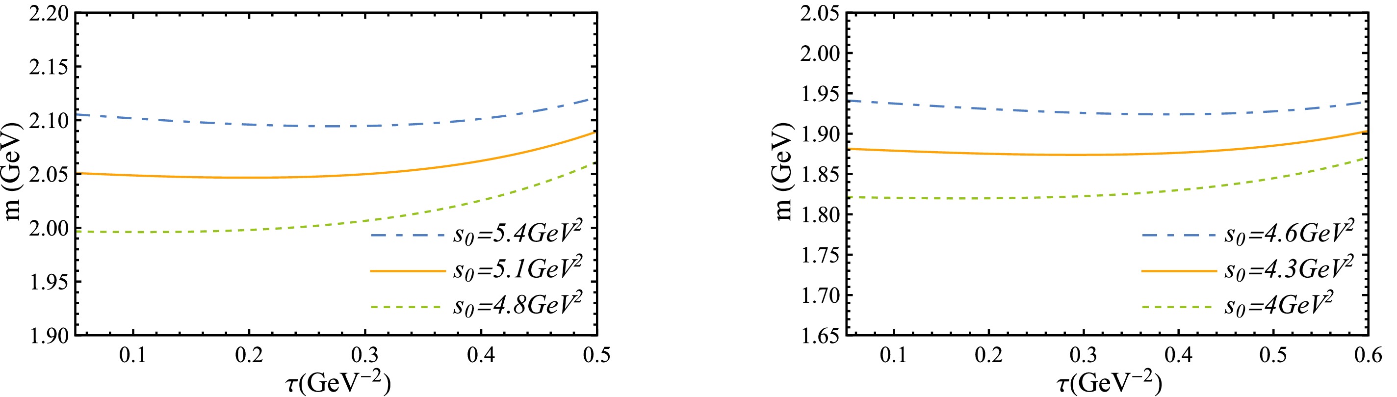
Figure A1. (color online) Mass predictions for the current
$ \eta_1^\mu $ (left) and$ \eta_2^\mu $ (right).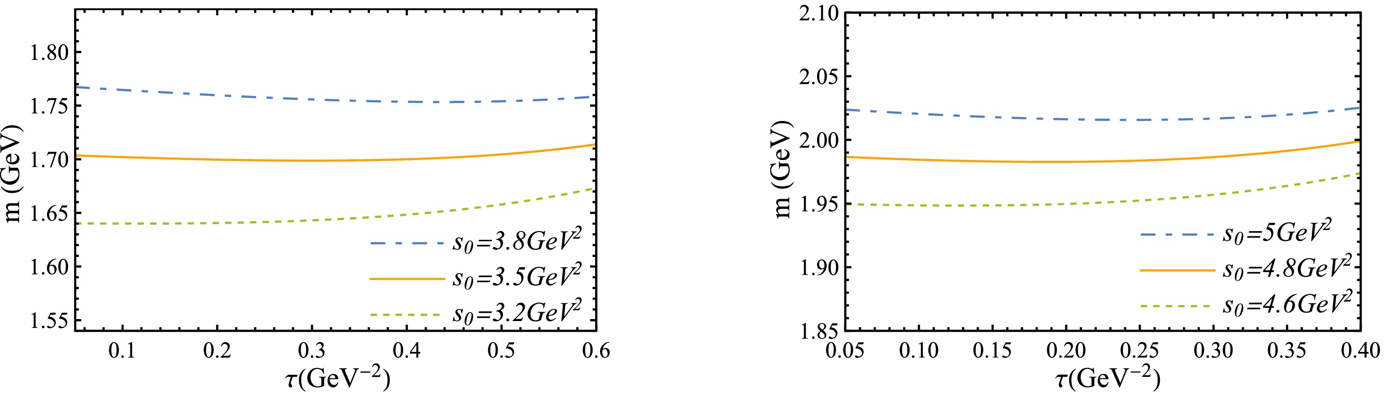
Figure A2. (color online) Mass predictions for the current
$ \eta_3^\mu $ (left) and$ \eta_4^\mu $ (right).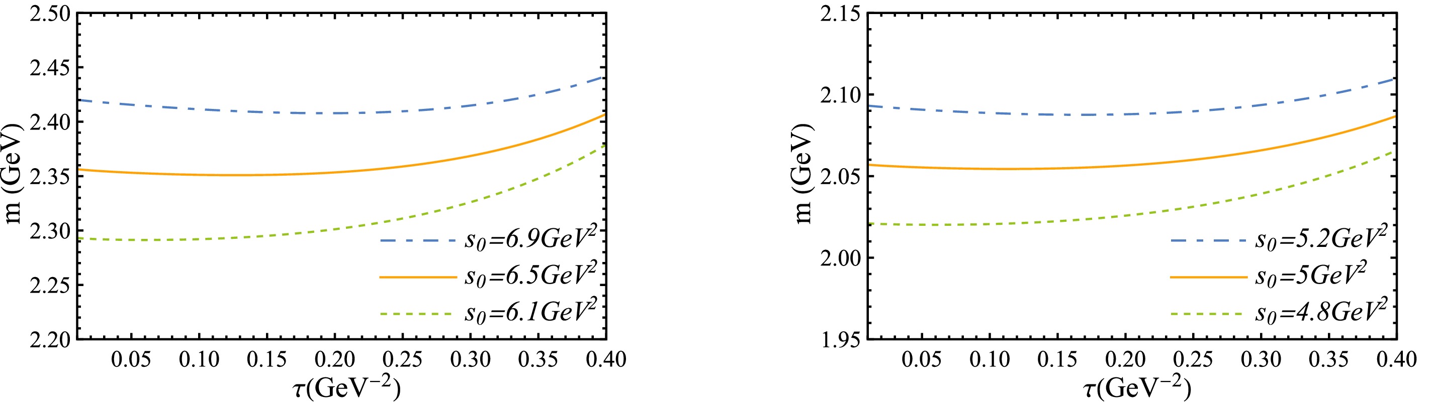
Figure A3. (color online) Mass predictions for the current
$ \eta_5^\mu $ (left) and$ \eta_6^\mu $ (right).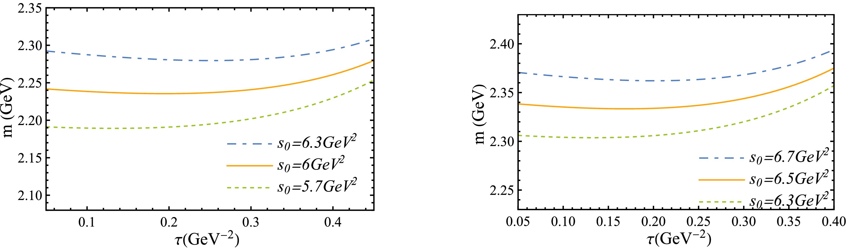
Figure A4. (color online) Mass predictions for the current
$ \eta_7^\mu $ (left) and$ \eta_8^\mu $ (right).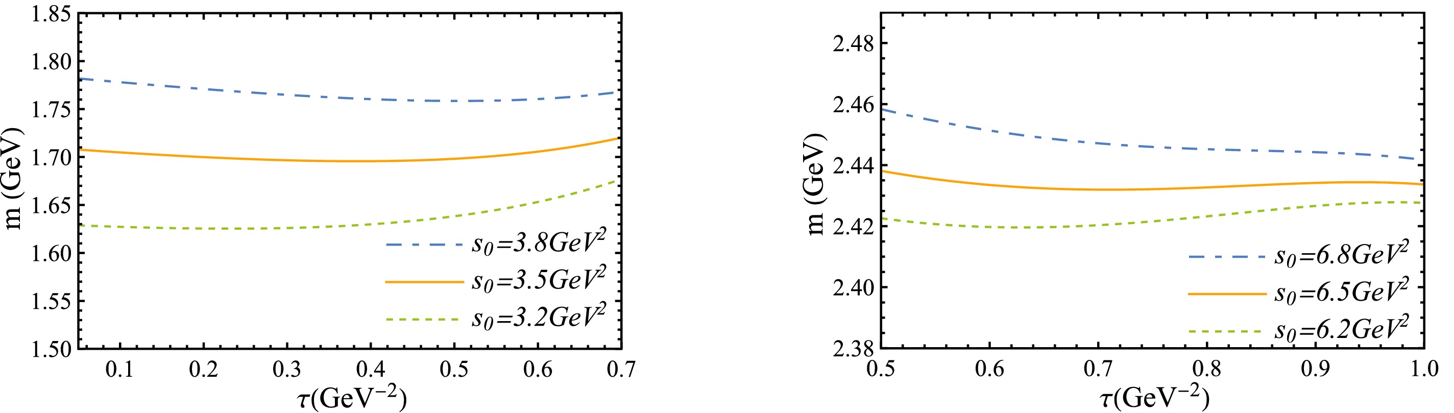
Figure A5. (color online) Mass predictions for the current
$ J_1^{\mu} $ (left) and$ J_2^{\mu\nu} $ (right). -
Renormalized operator current
$ J_2^{\mu\nu} $ :$ \begin{aligned}[b] \left(\epsilon^{\mu\nu\rho\sigma}\,\bar{u}\gamma^5\gamma_\rho d\, \bar{d}\gamma_\sigma u\right)_r=\;&\epsilon^{\mu\nu\rho\sigma}\,\bigg[\left(Z_2^{-2}+\frac{5C_F}{8\pi^2\varepsilon}g^2\right)\bar{u}\gamma_\rho\gamma^5 d\, \bar{d}\gamma_\sigma u-\frac{g^2}{8\pi^2\varepsilon}\bar{u}\gamma^5\gamma_\rho T^n d\, \bar{d}\gamma_\sigma\gamma^5 T^n u\\ &-\frac{i}{48\pi^2\varepsilon}\epsilon_{\rho\sigma\beta\eta}\left(\bar{u}D_\alpha G^{\alpha\beta}\gamma^\eta u - \bar{d}D_\alpha G^{\alpha\beta}\gamma^\eta d\right)\bigg] \end{aligned} $
(A1) For
$ \eta_2^\mu $ and$ \eta_4^\mu $ , their renormalization can be obtained through linear combinations of the following renormalization currents:$ \begin{aligned}[b] \left(u_a^T C\sigma^{\mu\nu}\gamma^5 d_b \, \bar{u}_a\gamma_\nu\gamma^5C\bar{d}^T_b\right)_r=\;&\left(Z_2^{-2} - \frac{4C_A^2-7}{32\pi^2\varepsilon C_A}g^2\right)u_a^T C\sigma^{\mu\nu}\gamma^5 d_b \, \bar{u}_a\gamma_\nu\gamma^5C\bar{d}^T_b-\frac{3g^2}{32\pi^2\varepsilon} u_a^T C\sigma^{\mu\nu}\gamma^5 d_b \, \bar{u}_b\gamma_\nu\gamma^5C\bar{d}^T_a\\ &-\frac{3iC_Ag^2}{32\pi^2\varepsilon}u_a^T C d_b \, \bar{u}_a\gamma^\mu C\bar{d}^T_b + \frac{3ig^2}{32\pi^2\varepsilon}u_a^T C d_b \, \bar{u}_b\gamma^\mu C\bar{d}^T_a \end{aligned} $
(A2) $ \begin{aligned}[b] \left(u_a^T C\sigma^{\mu\nu}\gamma^5 d_b \,\bar{u}_b\gamma_\nu\gamma^5C\bar{d}^T_a\right)_r=\;&\left(Z_2^{-2} - \frac{4C_A^2-7}{32\pi^2\varepsilon C_A}g^2\right)u_a^T C\sigma^{\mu\nu}\gamma^5 d_b \,\bar{u}_b\gamma_\nu\gamma^5C\bar{d}^T_a-\frac{3g^2}{32\pi^2\varepsilon} u_a^T C\sigma^{\mu\nu}\gamma^5 d_b \, \bar{u}_a\gamma_\nu\gamma^5C\bar{d}^T_b\\ &+\frac{3iC_Ag^2}{32\pi^2\varepsilon}u_a^T C d_b \, \bar{u}_b\gamma^\mu C\bar{d}^T_a - \frac{3ig^2}{32\pi^2\varepsilon}u_a^T C d_b \, \bar{u}_a\gamma^\mu C\bar{d}^T_b -\frac{1}{48\pi^2\varepsilon}\left(\bar{u}D^\alpha G_{\alpha\beta}\sigma^{\beta\mu}u - \bar{d}D^\alpha G_{\alpha\beta}\sigma^{\beta\mu}d\right)\\ &-\frac{i}{16\pi^2\varepsilon}\left(\bar{u}D_\alpha G^{\alpha\mu}u - \bar{d}D_\alpha G^{\alpha\mu}d\right) \end{aligned} $
(A3) By replacing the d quark with an s quark, the renormalization of operator currents
$ \eta_6^\mu $ and$ \eta_8^\mu $ can be obtained. -
$ \begin{aligned}[b] \Pi^V_{\eta_1}=\;&q^8\left[ \left(-\frac{79 g_s^2}{2654208 \pi ^8}-\frac{1}{18432 \pi ^6}\right) \log \left(-\frac{q^2}{\mu ^2}\right)-\frac{5 g_s^2 }{1327104 \pi ^8}\log ^2\left(-\frac{q^2}{\mu ^2}\right)\right] +q^4\frac{ g_s^2 }{18432 \pi ^6}\log \left(-\frac{q^2}{\mu ^2}\right) \langle GG \rangle\\&-q^2\frac{ 1}{18 \pi ^2}\log \left(-\frac{q^2}{\mu ^2}\right) \langle \bar{q}q \rangle ^2+\frac{1}{12 \pi ^2}\log \left(-\frac{q^2}{\mu ^2}\right) \langle \bar{q}q \rangle \langle \bar{q}Gq \rangle +\frac{1}{q^2}\left(\frac{5 g_s^2 }{864 \pi ^2}\langle GG \rangle \langle \bar{q}q \rangle ^2-\frac{1}{48 \pi ^2}\langle \bar{q}Gq \rangle ^2\right)\\ &+\frac{1}{q^4}\left(-\frac{g_s^2}{576 \pi ^2} \langle GG \rangle \langle \bar{q}q \rangle \langle \bar{q}Gq \rangle -\frac{32}{81} g_s^2 \langle \bar{q}q \rangle ^4\right) \end{aligned} $
$ \begin{aligned}[b] \Pi^V_{\eta_2}=\;& q^8\left[\frac{65 g_s^2 }{1769472 \pi ^8}\log ^2\left(-\frac{q^2}{\mu ^2}\right)+\left(-\frac{297929 g_s^2}{557383680 \pi ^8}-\frac{1}{6144 \pi ^6}\right) \log \left(-\frac{q^2}{\mu ^2}\right)\right]-q^4 \frac{11 g_s }{18432 \pi ^6}\log \left(-\frac{q^2}{\mu ^2}\right) \langle GG \rangle \\&-q^2 \frac{1}{6 \pi ^2}\log \left(-\frac{q^2}{\mu ^2}\right) \langle \bar{q}q \rangle ^2+\frac{1}{4 \pi ^2}\log \left(-\frac{q^2}{\mu ^2}\right) \langle \bar{q}q \rangle \langle \bar{q}Gq \rangle +\frac{1}{q^2}\left(-\frac{5 g_s^2 }{864 \pi ^2}\langle GG \rangle \langle \bar{q}q \rangle ^2-\frac{1}{16 \pi ^2}\langle \bar{q}Gq \rangle ^2\right)\\ &+\frac{1}{q^4}\left(\frac{g_s^2 }{576 \pi ^2}\langle GG \rangle \langle \bar{q}q \rangle \langle \bar{q}Gq \rangle -\frac{32 g_s^2}{27} \langle \bar{q}q \rangle ^4\right) \end{aligned} $
$ \begin{aligned}[b] \Pi^V_{\eta_3}=\;&q^8\left[\frac{5 g_s^2 }{884736 \pi ^8}\log ^2\left(-\frac{q^2}{\mu ^2}\right)+q^8 \left(-\frac{3503 g_s^2}{39813120 \pi ^8}-\frac{1}{36864 \pi ^6}\right) \log \left(-\frac{q^2}{\mu ^2}\right)\right]-q^4 \frac{g_s^2 }{18432 \pi ^6}\log \left(-\frac{q^2}{\mu ^2}\right) \langle GG \rangle \\&-q^2 \frac{1}{36 \pi ^2} \log \left(-\frac{q^2}{\mu ^2}\right) \langle \bar{q}q \rangle ^2+\frac{1}{24 \pi ^2}\log \left(-\frac{q^2}{\mu ^2}\right) \langle \bar{q}q \rangle \langle \bar{q}Gq \rangle +\frac{1}{q^2}\left(-\frac{5 g_s^2 }{864 \pi ^2}\langle GG \rangle \langle \bar{q}q \rangle ^2-\frac{1}{96 \pi ^2}\langle \bar{q}Gq \rangle ^2\right)\\ &+\frac{1}{q^4}\left(\frac{g_s^2 }{576 \pi ^2}\langle GG \rangle \langle \bar{q}q \rangle \langle \bar{q}Gq \rangle -\frac{16}{81} g_s^2 \langle \bar{q}q \rangle ^4\right) \end{aligned} $
$ \begin{aligned}[b] \Pi^V_{\eta_4}=\;& q^8\left[\frac{5 g_s^2 }{1769472 \pi ^8}\log ^2\left(-\frac{q^2}{\mu ^2}\right)+ \left(-\frac{26021 g_s^2}{557383680 \pi ^8}-\frac{1}{12288 \pi ^6}\right) \log \left(-\frac{q^2}{\mu ^2}\right)\right]-q^4\frac{ g_s^2 }{18432 \pi ^6}\log \left(-\frac{q^2}{\mu ^2}\right) \langle GG \rangle \\&-q^2\frac{1}{12 \pi ^2} \log \left(-\frac{q^2}{\mu ^2}\right) \langle \bar{q}q \rangle ^2+\frac{1}{8 \pi ^2}\log \left(-\frac{q^2}{\mu ^2}\right) \langle \bar{q}q \rangle \langle \bar{q}Gq \rangle +\frac{1}{q^2}\left(\frac{5 g_s^2 }{864 \pi ^2}\langle GG \rangle \langle \bar{q}q \rangle ^2-\frac{1}{32 \pi ^2}\langle \bar{q}Gq \rangle ^2\right)\\ &+\frac{1}{q^4}\left(-\frac{g_s^2 }{576 \pi ^2}\langle GG \rangle \langle \bar{q}q \rangle \langle \bar{q}Gq \rangle-\frac{16}{27} g_s^2 \langle \bar{q}q \rangle ^4\right) \end{aligned} $
$ \begin{aligned}[b] \Pi^V_{\eta_5}=\;&q^8 \left[\left(-\frac{2243 g_s^2}{79626240 \pi ^8}-\frac{1}{18432 \pi ^6}\right) \log \left(-\frac{q^2}{\mu ^2}\right)-\frac{7 g_s^2 }{1769472 \pi ^8}\log ^2\left(-\frac{q^2}{\mu ^2}\right)\right]+q^6\frac{17 m_s^2 }{7680 \pi ^6}\log \left(-\frac{q^2}{\mu ^2}\right)+q^4 \log \left(-\frac{q^2}{\mu ^2}\right) \\ &\times\left(-\frac{m_s \langle \bar{s}s\text{}\rangle }{48 \pi ^4}+\frac{m_s \langle \bar{q}q \rangle }{96 \pi ^4}+\frac{g_s^2 \langle GG \rangle }{18432 \pi ^6}\right)+q^2 \log \left(-\frac{q^2}{\mu ^2}\right) \left(\frac{m_s \langle \bar{s}\text{G}s\text{}\rangle }{96 \pi ^4}-\frac{\langle \bar{q}q \rangle \langle \bar{s}s\text{}\rangle }{9 \pi ^2}+\frac{\langle \bar{s}s\text{}\rangle ^2}{36 \pi ^2}-\frac{m_s \langle \bar{q}Gq \rangle }{48 \pi ^4}+\frac{\langle \bar{q}q \rangle ^2}{36 \pi ^2}-\frac{g_s^2 m_s^2 \langle GG \rangle }{4608 \pi ^6}\right)\\ &+\log \left(-\frac{q^2}{\mu ^2}\right) \left(\frac{\langle \bar{q}q \rangle \langle \bar{s}\text{G}s\text{}\rangle }{12 \pi ^2}-\frac{\langle \bar{s}s\text{}\rangle \langle \bar{s}\text{G}s\text{}\rangle }{24 \pi ^2}+\frac{\langle \bar{s}s\text{}\rangle \langle \bar{q}Gq \rangle }{12 \pi ^2}+\frac{m_s^2 \langle \bar{q}q \rangle \langle \bar{s}s\text{}\rangle }{2 \pi ^2}-\frac{m_s^2 \langle \bar{s}s\text{}\rangle ^2}{24 \pi ^2}-\frac{g_s^2 m_s \langle GG \rangle \langle \bar{q}q \rangle }{256 \pi ^4}-\frac{\langle \bar{q}q \rangle \langle \bar{q}Gq \rangle }{24 \pi ^2}+\frac{m_s^2 \langle \bar{q}q \rangle ^2}{6 \pi ^2}\right)\\ &+\frac{1}{q^2}\left(-\frac{\langle \bar{q}Gq \rangle \langle \bar{s}\text{G}s\text{}\rangle }{24 \pi ^2}-\frac{m_s^2 \langle \bar{q}q \rangle \langle \bar{s}\text{G}s\text{}\rangle }{6 \pi ^2}\right.\left.+\frac{\langle \bar{s}\text{G}s\text{}\rangle ^2}{96 \pi ^2}\right.\left.+\frac{5 g_s^2 \langle GG \rangle \langle \bar{q}q \rangle \langle \bar{s}s\text{}\rangle }{864 \pi ^2}-\frac{m_s^2 \langle \bar{s}s\text{}\rangle \langle \bar{q}Gq \rangle }{4 \pi ^2}-\frac{4}{9} m_s \langle \bar{q}q \rangle \langle \bar{s}s\text{}\rangle ^2-\frac{2}{3} m_s \langle \bar{q}q \rangle ^2 \langle \bar{s}s\text{}\rangle\right.\\ &\left. +\frac{5 g_s^2 m_s \langle GG \rangle \langle \bar{q}Gq \rangle }{4608 \pi ^4}+\frac{\langle \bar{q}Gq \rangle ^2}{96 \pi ^2}\right)+\frac{1}{q^4}\left(-\frac{g_s^2 \langle GG \rangle \langle \bar{q}q \rangle \langle \bar{s}\text{G}s\text{}\rangle }{1152 \pi ^2}-\frac{m_s^2 \langle \bar{q}Gq \rangle \langle \bar{s}\text{G}s\text{}\rangle }{24 \pi ^2}\right.+\frac{2}{9} m_s \langle \bar{q}q \rangle ^2 \langle \bar{s}\text{G}s\text{}\rangle -\frac{1}{9} m_s \langle \bar{q}q \rangle \langle \bar{s}s\text{}\rangle \langle \bar{s}\text{G}s\text{}\rangle \\ &-\frac{g_s^2 \langle GG \rangle \langle \bar{s}s\text{}\rangle \langle \bar{q}Gq \rangle }{1152 \pi ^2}-\frac{32}{81} g_s^2 \langle \bar{q}q \rangle ^2 \langle \bar{s}s\text{}\rangle ^2-\frac{1}{9} m_s \langle \bar{s}s\text{}\rangle ^2 \langle \bar{q}Gq \rangle +\frac{5}{9} m_s \langle \bar{q}q \rangle \langle \bar{s}s\text{}\rangle \langle \bar{q}Gq \rangle +\frac{m_s^2 \langle \bar{q}Gq \rangle ^2}{24 \pi ^2}\Bigg) \end{aligned} $
$ \begin{aligned}[b] \Pi^V_{\eta_6}=\;&q^8\left[ \frac{65 g_s^2 }{1769472 \pi ^8}\log ^2\left(-\frac{q^2}{\mu ^2}\right)+ \left(-\frac{297929 g_s^2}{557383680 \pi ^8}-\frac{1}{6144 \pi ^6}\right) \log \left(-\frac{q^2}{\mu ^2}\right)\right]+ q^6\frac{17 m_s^2 }{2560 \pi ^6}\log \left(-\frac{q^2}{\mu ^2}\right)+q^4 \log \left(-\frac{q^2}{\mu ^2}\right)\\&\times \left(-\frac{m_s \langle \bar{s}s\text{}\rangle }{16 \pi ^4}+\frac{m_s \langle \bar{q}q \rangle }{32 \pi ^4}-\frac{11 g_s^2 \langle GG \rangle }{18432 \pi ^6}\right)+q^2 \log \left(-\frac{q^2}{\mu ^2}\right) \left(\frac{m_s \langle \bar{s}\text{G}s\text{}\rangle }{32 \pi ^4}-\frac{\langle \bar{q}q \rangle \langle \bar{s}s\text{}\rangle }{3 \pi ^2}+\frac{\langle \bar{s}s\text{}\rangle ^2}{12 \pi ^2}-\frac{m_s \langle \bar{q}Gq \rangle }{16 \pi ^4}+\frac{\langle \bar{q}q \rangle ^2}{12 \pi ^2} + \frac{109 g_s^2 m_s^2 \langle GG \rangle }{18432 \pi ^6} \right)\\ &+\log \left(-\frac{q^2}{\mu ^2}\right) \Bigg(\frac{\langle \bar{q}q \rangle \langle \bar{s}\text{G}s\text{}\rangle }{4 \pi ^2}-\frac{\langle \bar{s}s\text{}\rangle \langle \bar{s}\text{G}s\text{}\rangle }{8 \pi ^2}-\frac{5 g_s^2 m_s \langle GG \rangle \langle \bar{s}s\text{}\rangle }{256 \pi ^4}+\frac{\langle \bar{s}s\text{}\rangle \langle \bar{q}Gq \rangle }{4 \pi ^2}+\frac{3 m_s^2 \langle \bar{q}q \rangle \langle \bar{s}s\text{}\rangle }{2 \pi ^2}-\frac{m_s^2 \langle \bar{s}s\text{}\rangle ^2}{8 \pi ^2}+\frac{3 g_s^2 m_s \langle GG \rangle \langle \bar{q}q \rangle }{128 \pi ^4}\\&-\frac{\langle \bar{q}q \rangle \langle \bar{q}Gq \rangle }{8 \pi ^2}+\frac{m_s^2 \langle \bar{q}q \rangle ^2}{2 \pi ^2}\Bigg)+\frac{1}{q^2}\Bigg(\frac{25 g_s^2 m_s \langle GG \rangle \langle \bar{s}\text{G}s\text{}\rangle }{4608 \pi ^4}-\frac{\langle \bar{q}Gq \rangle \langle \bar{s}\text{G}s\text{}\rangle }{8 \pi ^2}-\frac{m_s^2 \langle \bar{q}q \rangle \langle \bar{s}\text{G}s\text{}\rangle }{2 \pi ^2}+\frac{\langle \bar{s}\text{G}s\text{}\rangle ^2}{32 \pi ^2}-\frac{5 g_s^2 \langle GG \rangle \langle \bar{q}q \rangle \langle \bar{s}s\text{}\rangle }{144 \pi ^2}\\ &+\frac{25 g_s^2 \langle GG \rangle \langle \bar{s}s\text{}\rangle ^2}{1728 \pi ^2}-\frac{3 m_s^2 \langle \bar{s}s\text{}\rangle \langle \bar{q}Gq \rangle }{4 \pi ^2}-\frac{4}{3} m_s \langle \bar{q}q \rangle \langle \bar{s}s\text{}\rangle ^2-2 m_s \langle \bar{q}q \rangle ^2 \langle \bar{s}s\text{}\rangle -\frac{5 g_s^2 m_s \langle GG \rangle \langle \bar{q}Gq \rangle }{768 \pi ^4}+\frac{25 g_s^2 \langle GG \rangle \langle \bar{q}q \rangle ^2}{1728 \pi ^2}+\frac{\langle \bar{q}Gq \rangle ^2}{32 \pi ^2}\Bigg)\\&+\frac{1}{q^4}\Bigg(\frac{g_s^2 \langle GG \rangle \langle \bar{q}q \rangle \langle \bar{s}\text{G}s\text{}\rangle }{192 \pi ^2}-\frac{5 g_s^2 \langle GG \rangle \langle \bar{s}s\text{}\rangle \langle \bar{s}\text{G}s\text{}\rangle }{1152 \pi ^2}-\frac{m_s^2 \langle \bar{q}Gq \rangle \langle \bar{s}\text{G}s\text{}\rangle }{8 \pi ^2}+\frac{2}{3} m_s \langle \bar{q}q \rangle ^2 \langle \bar{s}\text{G}s\text{}\rangle -\frac{1}{3} m_s \langle \bar{q}q \rangle \langle \bar{s}s\text{}\rangle \langle \bar{s}\text{G}s\text{}\rangle\\& -\frac{5 g_s^2 m_s^2 \langle GG \rangle \langle \bar{s}s\text{}\rangle ^2}{1152 \pi ^2}+\frac{g_s^2 \langle GG \rangle \langle \bar{s}s\text{}\rangle \langle \bar{q}Gq \rangle }{192 \pi ^2}-\frac{32}{27} g_s^2 \langle \bar{q}q \rangle ^2 \langle \bar{s}s\text{}\rangle ^2-\frac{1}{3} m_s \langle \bar{s}s\text{}\rangle ^2 \langle \bar{q}Gq \rangle +\frac{5}{3} m_s \langle \bar{q}q \rangle \langle \bar{s}s\text{}\rangle \langle \bar{q}Gq \rangle \\ &-\frac{5 g_s^2 \langle GG \rangle \langle \bar{q}q \rangle \langle \bar{q}Gq \rangle }{1152 \pi ^2}+\frac{m_s^2 \langle \bar{q}Gq \rangle ^2}{8 \pi ^2}\Bigg)\end{aligned} $
$ \begin{aligned}[b] \Pi^V_{\eta_7}=\;& q^8\left[\frac{5 g_s^2 }{1769472 \pi ^8}\log ^2\Bigg(-\frac{q^2}{\mu ^2}\Bigg)+ \Bigg(-\frac{3503 g_s^2}{79626240 \pi ^8}-\frac{1}{36864 \pi ^6}\Bigg) \log \Bigg(-\frac{q^2}{\mu ^2}\Bigg)\right]+q^6 \frac{17 m_s^2 }{15360 \pi ^6}\log \Bigg(-\frac{q^2}{\mu ^2}\Bigg)+q^4 \log \Bigg(-\frac{q^2}{\mu ^2}\Bigg)\\ &\times \Bigg(-\frac{m_s \langle \bar{s}s\text{}\rangle }{96 \pi ^4}+\frac{m_s \langle \bar{q}q \rangle }{192 \pi ^4}-\frac{g_s^2 \langle GG \rangle }{18432 \pi ^6}\Bigg) +q^2 \log \Bigg(-\frac{q^2}{\mu ^2}\Bigg) \Bigg(\frac{m_s \langle \bar{s}\text{G}s\text{}\rangle }{192 \pi ^4}-\frac{\langle \bar{q}q \rangle \langle \bar{s}s\text{}\rangle }{18 \pi ^2}+\frac{\langle \bar{s}s\text{}\rangle ^2}{72 \pi ^2}-\frac{m_s \langle \bar{q}Gq \rangle }{96 \pi ^4}+\frac{\langle \bar{q}q \rangle ^2}{72 \pi ^2}+\frac{g_s^2 m_s^2 \langle GG \rangle }{4608 \pi ^6}\Bigg)\\ &+\log \Bigg(-\frac{q^2}{\mu ^2}\Bigg) \Bigg(\frac{\langle \bar{q}q \rangle \langle \bar{s}\text{G}s\text{}\rangle }{24 \pi ^2}-\frac{\langle \bar{s}s\text{}\rangle \langle \bar{s}\text{G}s\text{}\rangle }{48 \pi ^2}+\frac{\langle \bar{s}s\text{}\rangle \langle \bar{q}Gq \rangle }{24 \pi ^2}+\frac{m_s^2 \langle \bar{q}q \rangle \langle \bar{s}s\text{}\rangle }{4 \pi ^2}-\frac{m_s^2 \langle \bar{s}s\text{}\rangle ^2}{48 \pi ^2}+\frac{g_s^2 m_s \langle GG \rangle \langle \bar{q}q \rangle }{256 \pi ^4}-\frac{\langle \bar{q}q \rangle \langle \bar{q}Gq \rangle }{48 \pi ^2}+\frac{m_s^2 \langle \bar{q}q \rangle ^2}{12 \pi ^2}\Bigg)\\ &+\frac{1}{q^2}\Bigg(-\frac{\langle \bar{q}Gq \rangle \langle \bar{s}\text{G}s\text{}\rangle }{48 \pi ^2}-\frac{m_s^2 \langle \bar{q}q \rangle \langle \bar{s}\text{G}s\text{}\rangle }{12 \pi ^2}+\frac{\langle \bar{s}\text{G}s\text{}\rangle ^2}{192 \pi ^2}+\frac{5 g_s^2 \langle GG \rangle \langle \bar{q}q \rangle \langle \bar{s}s\text{}\rangle }{864 \pi ^2}-\frac{m_s^2 \langle \bar{s}s\text{}\rangle \langle \bar{q}Gq \rangle }{8 \pi ^2}-\frac{2}{9} m_s \langle \bar{q}q \rangle \langle \bar{s}s\text{}\rangle ^2-\frac{1}{3} m_s \langle \bar{q}q \rangle ^2 \langle \bar{s}s\text{}\rangle\\ & -\frac{5 g_s^2 m_s \langle GG \rangle \langle \bar{q}Gq \rangle }{4608 \pi ^4}+\frac{\langle \bar{q}Gq \rangle ^2}{192 \pi ^2}\Bigg)+\frac{1}{q^4}\Bigg(-\frac{m_s^2 \langle \bar{q}Gq \rangle \langle \bar{s}\text{G}s\text{}\rangle }{48 \pi ^2}+\frac{1}{9} m_s \langle \bar{q}q \rangle ^2 \langle \bar{s}\text{G}s\text{}\rangle -\frac{1}{18} m_s \langle \bar{q}q \rangle \langle \bar{s}s\text{}\rangle \langle \bar{s}\text{G}s\text{}\rangle \\ &+\frac{g_s^2 \langle GG \rangle \langle \bar{s}s\text{}\rangle \langle \bar{q}Gq \rangle }{1152 \pi ^2}-\frac{16}{81} g_s^2 \langle \bar{q}q \rangle ^2 \langle \bar{s}s\text{}\rangle ^2-\frac{1}{18} m_s \langle \bar{s}s\text{}\rangle ^2 \langle \bar{q}Gq \rangle +\frac{5}{18} m_s \langle \bar{q}q \rangle \langle \bar{s}s\text{}\rangle \langle \bar{q}Gq \rangle +\frac{g_s^2 \langle GG \rangle \langle \bar{q}q \rangle \langle \bar{q}Gq \rangle }{1152 \pi ^2}+\frac{m_s^2 \langle \bar{q}Gq \rangle ^2}{48 \pi ^2}\Bigg) \end{aligned} $
$ \begin{aligned}[b] \Pi^V_{\eta_8}=\;&q^8 \left[\frac{5 g_s^2 }{1769472 \pi ^8}\log ^2\Bigg(-\frac{q^2}{\mu ^2}\Bigg)+ \Bigg(-\frac{26021 g_s^2}{557383680 \pi ^8}-\frac{1}{12288 \pi ^6}\Bigg) \log \Bigg(-\frac{q^2}{\mu ^2}\Bigg)\right]+ q^6\frac{17 m_s^2 }{5120 \pi ^6}\log \Bigg(-\frac{q^2}{\mu ^2}\Bigg)+q^4 \log \Bigg(-\frac{q^2}{\mu ^2}\Bigg) \\ &\times\Bigg(-\frac{m_s \langle \bar{s}s\text{}\rangle }{32 \pi ^4}+\frac{m_s \langle \bar{q}q \rangle }{64 \pi ^4}-\frac{g_s^2 \langle GG \rangle }{18432 \pi ^6}\Bigg)+q^2 \log \Bigg(-\frac{q^2}{\mu ^2}\Bigg) \Bigg(\frac{m_s \langle \bar{s}\text{G}s\text{}\rangle }{64 \pi ^4}-\frac{\langle \bar{q}q \rangle \langle \bar{s}s\text{}\rangle }{6 \pi ^2}+\frac{\langle \bar{s}s\text{}\rangle ^2}{24 \pi ^2}-\frac{m_s \langle \bar{q}Gq \rangle }{32 \pi ^4}+\frac{\langle \bar{q}q \rangle ^2}{24 \pi ^2}+\frac{17 g_s^2 m_s^2 \langle GG \rangle }{18432 \pi ^6}\Bigg)\\ &+\log \Bigg(-\frac{q^2}{\mu ^2}\Bigg) \Bigg(\frac{\langle \bar{q}q \rangle \langle \bar{s}\text{G}s\text{}\rangle }{8 \pi ^2}-\frac{\langle \bar{s}s\text{}\rangle \langle \bar{s}\text{G}s\text{}\rangle }{16 \pi ^2}-\frac{g_s^2 m_s \langle GG \rangle \langle \bar{s}s\text{}\rangle }{256 \pi ^4}+\frac{\langle \bar{s}s\text{}\rangle \langle \bar{q}Gq \rangle }{8 \pi ^2}+\frac{3 m_s^2 \langle \bar{q}q \rangle \langle \bar{s}s\text{}\rangle }{4 \pi ^2}-\frac{m_s^2 \langle \bar{s}s\text{}\rangle ^2}{16 \pi ^2}-\frac{\langle \bar{q}q \rangle \langle \bar{q}Gq \rangle }{16 \pi ^2}+\frac{m_s^2 \langle \bar{q}q \rangle ^2}{4 \pi ^2}\Bigg)\\ &+\frac{1}{q^2}\Bigg(\frac{5 g_s^2 m_s \langle GG \rangle \langle \bar{s}\text{G}s\text{}\rangle }{4608 \pi ^4}-\frac{\langle \bar{q}Gq \rangle \langle \bar{s}\text{G}s\text{}\rangle }{16 \pi ^2}-\frac{m_s^2 \langle \bar{q}q \rangle \langle \bar{s}\text{G}s\text{}\rangle }{4 \pi ^2}+\frac{\langle \bar{s}\text{G}s\text{}\rangle ^2}{64 \pi ^2}+\frac{5 g_s^2 \langle GG \rangle \langle \bar{s}s\text{}\rangle ^2}{1728 \pi ^2}-\frac{3 m_s^2 \langle \bar{s}s\text{}\rangle \langle \bar{q}Gq \rangle }{8 \pi ^2}-\frac{2}{3} m_s \langle \bar{q}q \rangle \langle \bar{s}s\text{}\rangle ^2\\ &-m_s \langle \bar{q}q \rangle ^2 \langle \bar{s}s\text{}\rangle +\frac{5 g_s^2 \langle GG \rangle \langle \bar{q}q \rangle ^2}{1728 \pi ^2}+\frac{\langle \bar{q}Gq \rangle ^2}{64 \pi ^2}\Bigg)+\frac{1}{q^4}\Bigg(-\frac{g_s^2 \langle GG \rangle \langle \bar{s}s\text{}\rangle \langle \bar{s}\text{G}s\text{}\rangle }{1152 \pi ^2}-\frac{m_s^2 \langle \bar{q}Gq \rangle \langle \bar{s}\text{G}s\text{}\rangle }{16 \pi ^2}+\frac{1}{3} m_s \langle \bar{q}q \rangle ^2 \langle \bar{s}\text{G}s\text{}\rangle \\ &-\frac{1}{6} m_s \langle \bar{q}q \rangle \langle \bar{s}s\text{}\rangle \langle \bar{s}\text{G}s\text{}\rangle -\frac{g_s^2 m_s^2 \langle GG \rangle \langle \bar{s}s\text{}\rangle ^2}{1152 \pi ^2}-\frac{16}{27} g_s^2 \langle \bar{q}q \rangle ^2 \langle \bar{s}s\text{}\rangle ^2-\frac{1}{6} m_s \langle \bar{s}s\text{}\rangle ^2 \langle \bar{q}Gq \rangle +\frac{5}{6} m_s \langle \bar{q}q \rangle \langle \bar{s}s\text{}\rangle \langle \bar{q}Gq \rangle \\ &-\frac{g_s^2 \langle GG \rangle \langle \bar{q}q \rangle \langle \bar{q}Gq \rangle }{1152 \pi ^2}+\frac{m_s^2 \langle \bar{q}Gq \rangle ^2}{16 \pi ^2}\Bigg) \end{aligned} $
$ \begin{aligned}[b] \Pi^V_{J_1}=\;& q^8 \left[\frac{25 g_s^2 }{14155776 \pi ^8}\log ^2\left(-\frac{q^2}{\mu ^2}\right)+ \left(-\frac{41221 g_s^2}{1114767360 \pi ^8}-\frac{11}{1179648 \pi ^6}\right) \log \left(-\frac{q^2}{\mu ^2}\right)\right]-q^4\frac{ g_s^2 }{32768 \pi ^6}\log \left(-\frac{q^2}{\mu ^2}\right) \langle GG \rangle \\ &+q^2 \frac{1}{128 \pi ^2}\log \left(-\frac{q^2}{\mu ^2}\right) \langle \bar{q}q\text{}\rangle ^2-\frac{3 }{256 \pi ^2}\log \left(-\frac{q^2}{\mu ^2}\right) \langle \bar{q}q\text{}\rangle \langle \bar{q}\text{G}q\text{}\rangle +\frac{1}{q^2}\left(\frac{3 }{1024 \pi ^2}\langle \bar{q}\text{G}q\text{}\rangle ^2+\frac{5 g_s^2}{1536 \pi ^2} \langle GG \rangle \langle \bar{q}q\text{}\rangle ^2\right)\\ &+\frac{1}{q^4}\frac{g_s^2 }{3072 \pi ^2 }\langle GG \rangle \langle \bar{q}q\text{}\rangle \langle \bar{q}\text{G}q\text{}\rangle \end{aligned} $
$ \begin{aligned}[b] \Pi^V_{J_2}=\;&q^8 \left[\left(-\frac{77 g_s^2}{2764800 \pi ^8}-\frac{1}{30720 \pi ^6}\right) \log \left(-\frac{q^2}{\mu ^2}\right)-\frac{g_s^2 }{829440 \pi ^8}\log ^2\left(-\frac{q^2}{\mu ^2}\right)\right]+q^4\frac{ g_s^2 }{3072 \pi ^6}\log \left(-\frac{q^2}{\mu ^2}\right) \langle GG \rangle\\ &+q^2 \left[ \left(-\frac{5 \gamma g_s^2 }{216 \pi ^4}-\frac{5 g_s^2 }{1296 \pi ^4}\right)\log \left(-\frac{q^2}{\mu ^2}\right)-\frac{5 g_s^2 }{216 \pi ^4}\log ^2\left(-\frac{q^2}{\mu ^2}\right) \right]\langle \bar{q}q \rangle ^2\\ &+\frac{1}{48 \pi ^2}\log \left(-\frac{q^2}{\mu ^2}\right) \langle \bar{q}q \rangle \langle \bar{q}Gq \rangle +\frac{1}{q^2}\left(-\frac{g_s^2 }{864 \pi ^2}\langle GG \rangle \langle \bar{q}q \rangle ^2-\frac{1}{192 \pi ^2}\langle \bar{q}Gq \rangle ^2\right)+\frac{1}{q^4}\frac{g_s^2 }{1728 \pi ^2 }\langle GG \rangle \langle \bar{q}q \rangle \langle \bar{q}Gq \rangle \end{aligned} $
-
The figure displays the comparison of the masses determined at NLO and LO. For
$ j_1^\mu $ and$ j_2^{\mu\nu} $ , the previous study also considered the zero mode contribution, therefore they are not compared here.
NLO QCD sum rules analysis of 1−+ tetraquark states
- Received Date: 2026-01-14
- Available Online: 2026-06-01
Abstract: We performed a next-to-leading-order (NLO) QCD sum rules analysis of the $1^{-+}$ light tetraquark states. By investigating various compact and molecular tetraquark currents, we extracted the mass spectra of the corresponding states, all of which lie above $1.7\,\text{GeV}$. We find multiple $1^{-+}$ states around $2.0\,\text{GeV}$ that match well with $\pi_{1}(2015)$, which makes us confident that $\pi_{1}(2015)$ is an excellent tetraquark candidate. In contrast, our calculations exclude the possibility that the $\pi_{1}(1400)$ is a tetraquark or hybrid-tetraquark mixture. This suggests that it may not exist, which is consistent with recent experimental results.


 DownLoad: