


 Abstract
 HTML
HTML Reference
 Related
 PDF
PDF


-
Ultrarelativistic heavy-ion collisions conducted at the relativistic heavy ion collider (RHIC) and large hadron collider (LHC) generate a novel state of matter referred to as the quark gluon plasma (QGP) [1, 2]. Investigating particles with high momentum is an essential method for clarifying the characteristics of QGP. These high-energy particles are produced by high-energy partons, which can be accurately calculated from perturbative quantum chromodynamics (pQCD) [3−6], rendering these hard probes highly effective for examining the properties of the medium. An essential feature of the medium-parton interaction is the phenomenon of energy loss in high energy nucleus-nucleus collisions, resulting in a suppressed hadron cross-section at high transverse momentum (
$ p_T $ ) relative to what is anticipated by a direct scaling of the cross-section in proton-proton collisions. This effect, termed jet quenching [7−11], is most effectively analyzed using the nuclear modification factor$ R_{AA} $ .$ R_{AA} $ is defined as the ratio of the particle spectrum in heavy-ion collisions to the product of proton-proton cross-section and nucleus-nucleus thickness overlapping function. This deviation from unity indicates nuclear medium effects.A commonly applied approach to calculate energy loss in QGP relies on the premise of weakly coupled scenarios between high-energy partons and the QGP. Within this scenario, high-energy partons traverse the medium along the light cone, losing energy via medium-induced gluon emission as a consequence of multiple collisions with the medium. This weakly coupled approach has been remarkably effective in describing the suppression of
$ R_{AA} $ as observed in nuclear collisions. However, in many of these models, elastic energy losses are perturbatively calculated and receive large contributions from soft momentum$ q\sim g_s T $ exchange with the medium, where$ g_s $ represents the QCD coupling. This is difficult to reconcile with the experimental discovery that the QGP produced in heavy-ion collisions is strongly coupled [12, 13]. The phenomenological coupling is so large that$ g_s T $ is almost comparable to the thermal kinetic energy. Therefore, this weak coupling approach may have certain limitations when dealing with strongly coupled QGP. Consequently, it is unclear if jet quenching can be understood from a non-perturbative or strongly coupled perspective. In this paper, we adopt a strongly coupled approach, assuming strong coupling between the medium and the parton; meanwhile, we introduce dependence on the background magnetic field and chemical potential and investigate jet quenching phenomena using gauge/gravity duality [14, 15].Gauge/gravity dualities present a broad collection of concepts asserting that gauge field theories in four-dimensional flat space are dual to gravity theories in curved space with an additional dimension. The anti-de sitter/conformal field theory (
$ \mathrm{AdS/CFT} $ ) correspondence [16−19] is a specific instance of gauge/gravity dualities. Since its introduction in the late 1990s, it has emerged as one of the most intensively researched areas in theoretical high-energy physics. The$ \mathrm{AdS/CFT} $ correspondence confirms that there is a certain relationship between the$ \mathrm{AdS}_{5}\times S^{5} $ space-time type$ \mathrm{IIB} $ string theory and$ {\cal{N}} $ = 4 supersymmetric Yang-Mills ($ \mathrm{SYM} $ ) gauge field theory in the (3+1)-dimensional Minkowski space-time. While$ {\cal{N}} $ = 4$ \mathrm{SYM} $ at zero temperature exhibits distinct differences from$ \mathrm{QCD} $ in various aspects, it can provide insights into certain qualitative characteristics of$ \mathrm{QCD} $ under the strongly coupled regime at finite temperature. Within the AdS/CFT correspondence, the features of the medium are embedded in the background metric of the associated string theory (e.g., the$ \mathrm{AdS}_{5} $ metric for$ {\cal{N}} $ = 4$ \mathrm{SYM} $ ), while the traits of diverse dynamic processes occurring within the medium are manifested through the behavior of classical strings in this background. According to the strong and weak correspondences in the$ \mathrm{AdS/CFT} $ , the strong coupling problem faced by four-dimensional CFT can be solved by the corresponding weak coupling method of the superstring theory. Thus far, researchers exploited the$ \mathrm{AdS/CFT} $ to explore various properties of QGP. For example, jet quenching parameters [20−23], ratio of shear viscosity to entropy density [24], phase transition [25−32], heavy quark potential [33−36], heavy quark energy loss [37−40], and light quark energy loss [41−46].This paper focuses on the effects of the constant magnetic field and chemical potential on holographic jet energy loss in high-energy nucleus-nucleus collisions at the RHIC/LHC. Recent studies have indicated that extremely high magnetic fields may be generated with magnitudes on the order of
$ eB\sim 70m_{\pi}^{2} $ in the initial stages of noncentral ultrarelativistic heavy ion collisions at LHC energies [47−50]. The generated magnetic field decreases rapidly; however, it remains influential in the initial stage of$ \mathrm{QGP} $ formation [47, 51]. This strong magnetic field affects the QCD phase transition [52−54], plasma evolution, and charge dynamics in strongly interacting matter [55−57]. The effect of a finite baryon chemical potential is small at LHC energy; however, it can be influential at various RHIC energies [58]. Both magnetic and chemical potentials can alter the properties of the partonic degrees of freedom of the QGP; therefore, it is interesting to study the corresponding response of jet quenching. Recent work has separately studied the effects of magnetic fields and chemical potential on parton energy loss [59, 60]. In this paper, we simultaneously analyze the effects of the magnetic field and chemical potential, revealing their strong correlations in impacting parton energy loss. Finally, using Bayesian inference, we discuss the phenomenological sensitivity of jet quenching observables to the magnetic field and chemical potential. In this study, we calculate the energy loss$ \mathrm{d}E/\mathrm{d}x $ and subsequently employ a Bayesian analysis approach. This enables us to not only investigate the effect of the magnetic field on jet quenching effects but also infer the range distribution of the magnetic field across different collision centralities at both RHIC and LHC energies.The remainder of this paper is organized as follows: In Sec. II, we review the next-to-leading order (NLO) pQCD parton model. A holographic model of the energy loss incorporating magnetic fields and chemical potentials is introduced in Sec. III. In Sec. IV, we determine the coupling constant in the model. In Sec. V, we describe the holographic jet energy loss in the background of a magnetic field and chemical potential. In Sec. VI, we show details of the Bayesian analysis, and in Sec. VII, we discuss the results. Finally, we present a summary and an outlook in Sec. VIII.
-
We provide a brief overview of the
$ \mathrm{pQCD} $ computations related to the NLO cross-sections for producing single inclusive hadrons at high transverse momentum$ p_{T} $ in$ p+p $ and$ A+A $ collisions, utilizing the concept of collinear factorization. -
We provide a brief overview of the
$ \mathrm{pQCD} $ computations related to the NLO cross-sections for producing single inclusive hadrons at high transverse momentum$ p_{T} $ in$ p+p $ and$ A+A $ collisions, utilizing the concept of collinear factorization. -
We provide a brief overview of the
$ \mathrm{pQCD} $ computations related to the NLO cross-sections for producing single inclusive hadrons at high transverse momentum$ p_{T} $ in$ p+p $ and$ A+A $ collisions, utilizing the concept of collinear factorization. -
The invariant cross-section for producing a single hadron with high transverse momentum in high-energy collisions can be factorized within the parton model. This factorization involves the convolution of collinear parton distribution functions (PDFs), hard scattering cross-sections, and fragmentation functions (FFs) [61]. The differential cross-section as a function of the hadron with transverse momentum
$ p_{T} $ and rapidity$ y_{h} $ is [62]$ \begin{aligned}[b]\frac{{\mathrm{{d}}}\sigma_{pp}^h}{\mathrm{d}y_h\mathrm{d}^2p_T}=\; & \sum\limits_{abcd}^{ }\int_{ }^{ }\mathrm{d}x_a\mathrm{d}x_bf_{a/p}(x_a,\mu^2)f_{b/p}(x_b,\mu^2) \\ & \times\frac{1}{\pi}\frac{\mathrm{d}\sigma_{ab\rightarrow cd}}{\mathrm{d}\hat{t}}\frac{D_c^h(z_c,\mu^2)}{z_c}+{\cal{O}}(\alpha_s^3).\end{aligned} $
(1) where
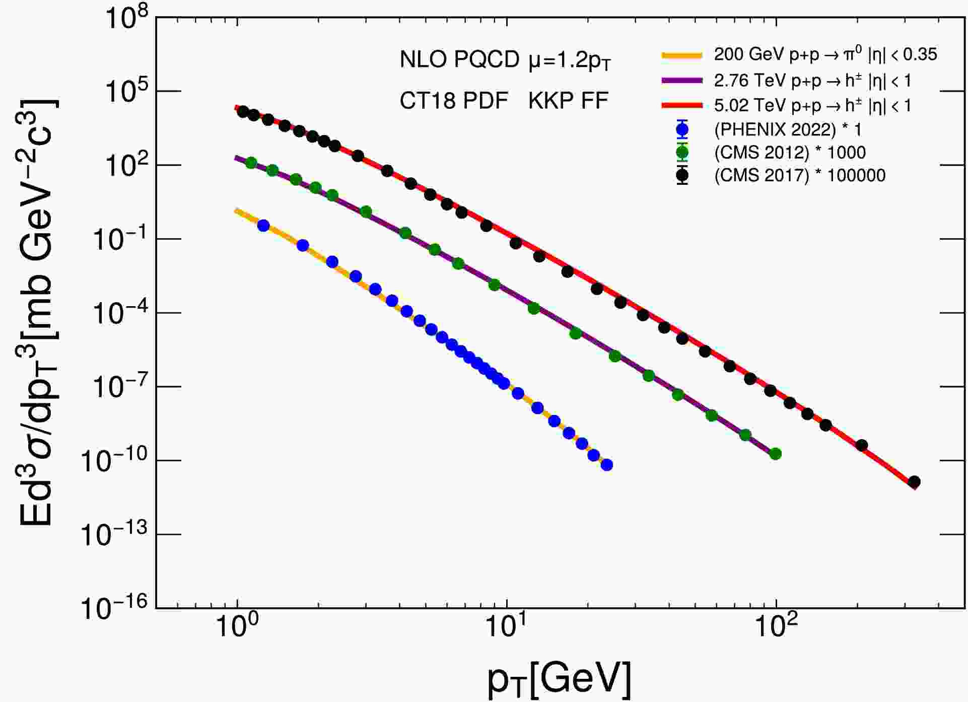
$ f_{a/p}(x_{a},\mu^{2}) $ and$ f_{b/p}(x_{b},\mu^{2}) $ represent the parton distribution functions obtained from$ \mathrm{CT18} $ [63] parametrization, while$ D_{c}^{h}(z_{c},\mu^{2}) $ represents the fragmentation function of the Kniehl-Kramer-Potter parametrization in vacuum from Ref. [64]. The LO partonic cross-section for the$ 2\rightarrow2 $ process$ ab\rightarrow cd $ is denoted by$ \mathrm{d}\sigma_{ab\rightarrow cd} $ . The NLO correction at$ {\cal{O}}(\alpha_{s}^{3}) $ contains virtual corrections to the$ 2\rightarrow2 $ cross-sections and$ 2\rightarrow3 $ tree-level cross-sections. We consider the renormalization scale of$ \mu=1.2\;p_{T}^{h} $ at RHIC and LHC to describe hadron production in vacuum.Figure 1 shows the NLO pQCD result on the hadron production cross-section in
$ p+p $ collisions compared with experimental data [65−67]. These numerical results confirm that the NLO pQCD parton model present a good description of the experimental data of single-hadron production at large$ p_{T} $ in$ p+p $ collision. -
The invariant cross-section for producing a single hadron with high transverse momentum in high-energy collisions can be factorized within the parton model. This factorization involves the convolution of collinear parton distribution functions (PDFs), hard scattering cross-sections, and fragmentation functions (FFs) [61]. The differential cross-section as a function of the hadron with transverse momentum
$ p_{T} $ and rapidity$ y_{h} $ is [62]$ \begin{aligned}[b]\frac{{\mathrm{{d}}}\sigma_{pp}^h}{\mathrm{d}y_h\mathrm{d}^2p_T}=\; & \sum\limits_{abcd}^{ }\int_{ }^{ }\mathrm{d}x_a\mathrm{d}x_bf_{a/p}(x_a,\mu^2)f_{b/p}(x_b,\mu^2) \\ & \times\frac{1}{\pi}\frac{\mathrm{d}\sigma_{ab\rightarrow cd}}{\mathrm{d}\hat{t}}\frac{D_c^h(z_c,\mu^2)}{z_c}+{\cal{O}}(\alpha_s^3).\end{aligned} $
(1) where
$ f_{a/p}(x_{a},\mu^{2}) $ and$ f_{b/p}(x_{b},\mu^{2}) $ represent the parton distribution functions obtained from$ \mathrm{CT18} $ [63] parametrization, while$ D_{c}^{h}(z_{c},\mu^{2}) $ represents the fragmentation function of the Kniehl-Kramer-Potter parametrization in vacuum from Ref. [64]. The LO partonic cross-section for the$ 2\rightarrow2 $ process$ ab\rightarrow cd $ is denoted by$ \mathrm{d}\sigma_{ab\rightarrow cd} $ . The NLO correction at$ {\cal{O}}(\alpha_{s}^{3}) $ contains virtual corrections to the$ 2\rightarrow2 $ cross-sections and$ 2\rightarrow3 $ tree-level cross-sections. We consider the renormalization scale of$ \mu=1.2\;p_{T}^{h} $ at RHIC and LHC to describe hadron production in vacuum.Figure 1 shows the NLO pQCD result on the hadron production cross-section in
$ p+p $ collisions compared with experimental data [65−67]. These numerical results confirm that the NLO pQCD parton model present a good description of the experimental data of single-hadron production at large$ p_{T} $ in$ p+p $ collision. -
In nucleus-nucleus collisions with a fixed impact parameter
$ \boldsymbol{b} $ , the single-inclusive hadron production spectra at high transverse momentum$ p_{T} $ can be expressed as (analogous to Eq. 1) [68−70]$ \begin{aligned}[b]\frac{\mathrm{d}N_{AB}^h(b)}{\mathrm{d}yd^2p_T}=\; & \sum\limits_{abcd}^{ }\int_{ }^{ }\mathrm{d}x_a\mathrm{d}x_bd^2rt_A(\boldsymbol{r})t_B(\boldsymbol{r}+\boldsymbol{b}) \\ & \times f_{a/A}(x_a,\mu^2,\boldsymbol{r})f_{b/B}(x_b,\mu^2,\boldsymbol{r}+\boldsymbol{b}) \\ & \times\frac{1}{\pi}\frac{\mathrm{d}\sigma_{ab\rightarrow cd}}{\mathrm{d}\hat{t}}\frac{D_c^h(z_c,\mu^2,\bigtriangleup E_c)}{z_c}+{\cal{O}}(\alpha_s^3).\end{aligned} $
(2) where
$ t_{A}(\boldsymbol{r}) $ and$ t_{B}(\boldsymbol{r}+\boldsymbol{b}) $ represent the projectile and target nuclear thickness functions normalized as$ \int_{ }^{ }\mathrm{d}^2rt_A(\boldsymbol{r})=A $ , with A denoting the mass number of the nucleus. We use the Woods-Saxon form for the nuclear density distribution.$ f_{a/A}(x_{a},\mu^{2},\boldsymbol{r}) $ represents the nuclear modified PDF [71−74] given by$ \begin{aligned}[b] f_{a/A}(x_{a},\mu^{2},\boldsymbol{r}) =\;&S_{a/A}(x_{a},\mu^{2},\boldsymbol{r})\bigg[\frac{Z}{A}f_{a/p}(x_{a},\mu^{2})\\ &+\bigg(1-\frac{Z}{A}f_{a/n}(x_{a},\mu^{2}\bigg)\bigg] , \end{aligned} $
(3) where Z represents the proton number of the nucleus.
$ S_{a/A}(x_{a},\mu^{2},\boldsymbol{r}) $ indicates the nuclear shadowing factor and modification of the nuclear PDF as compared to the simple isospin average using the PDF of a free proton$ f_{a/p}(x_{a},\mu^{2}) $ . The shadowing factor$ S_{a/A}(x_{a},\mu^{2},\boldsymbol{r}) $ takes the form [75−77]$ S_{a/A}(x_{a},\mu^{2},\boldsymbol{r}) =1+A\frac{t_{A}(\boldsymbol{r})\big[S_{a/A}(x_{a},\mu^{2})-1\big]}{\int d^{2}r[t_{A}(\boldsymbol{r})]} , $
(4) and we use the
$ \mathrm{EPPS21} $ parametrization for$ S_{a/A}(x_{a},\mu^{2}) $ [78]. Finally,$ D_{h/c}(z_{c},\mu^{2},\Delta E_{c}) $ represents the medium-modified fragmentation function given by [70, 79−82]$ D_{h/c}(z_{c},\mu^{2},\Delta E_{c}) =\frac{z_{c}^{\prime}}{z_{c}}D_{h/c}(z_{c}^{\prime},\mu^{2}) , $
(5) where
$ \Delta E_{c} $ represents the energy loss of parton c. Variable$ z_{c}=p_{T}/p_{Tc} $ represents the vacuum fragmentation momentum fraction of a hadron from parton c, while$ z_{c}^{\prime}=p_{T}/(p_{Tc}-\Delta E_{c}) $ corresponds to the in-medium case, where parton loses energy$ \Delta E_{c} $ prior to fragmentation. The calculation of$ \Delta E_{c} $ will be given in the next section from the holographic model. -
Based on the calculations in both
$ p+p $ and$ A+A $ collisions, the nuclear modification factor for single-inclusive hadron production in heavy-ion collisions can be computed following the approach in [83].$ R_{AA}(p_T)=\frac{\dfrac{\mathrm{d}N_{AA}}{\mathrm{d}y\mathrm{d}^2p_T}}{T_{AB}(\boldsymbol{b})\dfrac{\mathrm{d}\sigma_{pp}}{\mathrm{d}y\mathrm{d}^2p_T}}, $
(6) where
$ T_{AA}(\boldsymbol{b})=\int d^{2}\boldsymbol{r}t_{A}(\boldsymbol{r})t_{A}(\boldsymbol{r}+\boldsymbol{b}) $ defines the nuclear overlap function, which quantifies the geometric overlap of the two colliding nuclei at specific impact parameter$ \boldsymbol{b} $ for specific centrality. -
We introduce a holographic model with a magnetic field and chemical potential. Within the
$ \mathrm{AdS/CFT} $ correspondence, introducing a magnetic field and chemical potential into$ {\cal{N}} $ = 4$ \mathrm{SYM} $ can be achieved by endowing the black hole in the holographic dimension with charge. The resulting spacetime geometry is described by an AdS-RN black hole, whose dynamics are governed by [60, 84]$ I=\frac{1}{2\kappa^2}\int_{ }^{ }\mathrm{d}^5x\sqrt{-g}\left({\cal{R}}+\frac{12}{L^2}-\frac{L^2}{g_F^2}F_{\mu\nu}F^{\mu\nu}\right), $
(7) In this context,
$ \kappa_{4}^{2}=8\pi G $ , where G represents the gravitational constant and$ {\cal{R}} $ represents the Ricci scalar. Parameter L indicates the radius of the$ \mathrm{AdS} $ space, which, for simplicity, is normalized to unity ($ L=1 $ ) in the subsequent analysis. The effective dimensionless gauge coupling constant is denoted by$ g_{F} $ . The value of$ g_{F} $ is set to 1 [84]. Field strength tensor$ F_{\mu\nu} $ is expressed as$ F_{\mu\nu}=\partial_{\mu}A_{\nu}-\partial_{\nu}A_{\mu} $ , with$ A_{\mu } $ being the$ U(1) $ gauge field. The five-dimensional solution to the equations of motion derived from Eq. (7) is given by$ \mathrm{d}s^{2}=\frac{1}{z^{2}}\bigg(-f(z)\mathrm{d}t^{2}+\mathrm{d}\boldsymbol{x}^{2}+\frac{\mathrm{d}z^{2}}{f(z)}\bigg) , $
(8) with
$ f(z)=1-(1+Q^{2})\bigg(\frac{z}{z_{h}}\bigg)^{4}+Q^{2}\bigg(\frac{z}{z_{h}}\bigg)^{6} , $
(9) where
$ Q^{2}=\mu^{2}_{B}z_{h}^{2}+B^{2}z_{h}^{4} $ [85−87] is the charge of the black hole, and$ \mu_B $ and B represent the baryon chemical potential and background magnetic field, respectively. Eq. (9) is an approximate solution of Eq. (7). However, the specific form$ Q^{2}=\mu^{2}_{B}z_{h}^{2}+B^{2}z_{h}^{4} $ adopted in our computational framework constitutes an assumption introduced for$ Q^{2} $ to incorporate both magnetic field and chemical potential effects [85, 86]. This treatment in our work conducts a preliminary exploration of the feasibility of introducing a magnetic field and chemical potential through$ Q^{2} $ . Based on this assumption, setting both the magnetic field and chemical potential to zero enables the energy loss formulation to revert to the form presented in Ref. [41]; this characterizes energy loss in the absence of magnetic and chemical potential effects. As a pioneering study that applies holographic energy loss to investigate jet quenching phenomena, Ref. [41] serves as an important benchmark in this field. The chemical potential is associated with charge density [87]. Both the charge density and magnetic field originate from the same$ U(1) $ current, and therefore, the chemical potential and magnetic field can be consequently described within the same$ U(1) $ symmetry framework. t represents the time coordinate,$ \boldsymbol{x} $ represents the$ \mathrm{CFT} $ space coordinates on the boundary, and z represents the$ \mathrm{AdS} $ space coordinate. In addition,$ z=z_h $ represents the horizon near the boundary of the black hole, as shown in Fig. 2.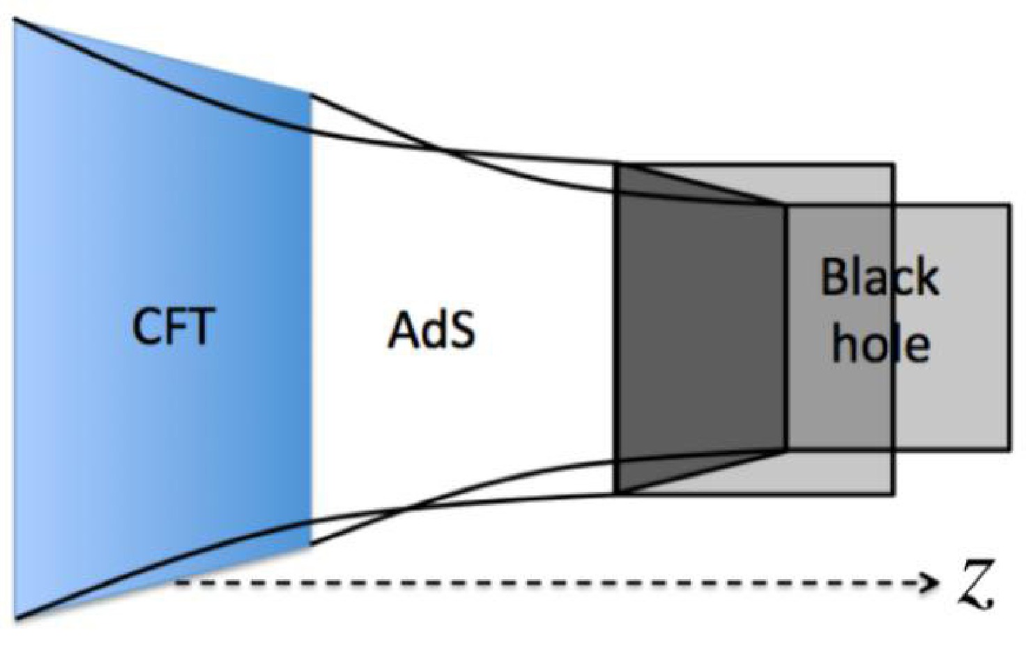
Figure 2. (color online) Illustration of the
$ \mathrm{AdS/CFT} $ correspondence. z represents the bulk coordinate.We use the Hawking formula of the black hole
$ T(z_{h},\mu_{B},B)=\frac{1}{\pi z_{h}}\left(1-\frac{Q^{2}}{2}\right). $
(10) For a given set of T,
$ \mu_{B} $ , and B, Eq. (10) yields four roots for$ z_{h} $ . However, the physically acceptable solution is the only one of these roots that is real and positive. Therefore, we only consider the branch with$ z_{h}>0 $ .In our calculations,
$ Q^{2} $ is defined as$ Q^{2} = \mu_{B}^{2}z_{h}^{2} + B^{2}z_{h}^{4} $ , which incorporates contributions from the magnetic field and chemical potential. As shown in Eq. (10),$ Q^{2} $ exhibits explicit temperature dependence. The energy loss calculation is temperature dependent; therefore, the temperature is provided by the CLVisc hydrodynamic framework [88, 89]. Our model effectively introduces the effect of the magnetic field and chemical potential on energy loss through their temperature-dependent coupling via$ Q^{2} $ . -
We apply the methodology presented in Refs. [41, 42] to investigate the effect of a magnetic field and chemical potential on the energy loss of light quarks using finite endpoint momentum shooting strings. In this approach, a specific classical string motion is considered, wherein the endpoint of the string starts near the horizon and moves towards the boundary while carrying certain energy and momentum. As the string rises, this energy and momentum gradually dissipate into the remaining part. Hence, this motion is called a finite-endpoint-momentum shooting string.
The AdS space-time metric Eq. (8) can be rewritten in the form (here,
$ \mathrm{d}x $ represents$ \mathrm{d}\boldsymbol{x} $ in Eq. (8))$ \mathrm{d}s^{2} =G_{tt}(z)\mathrm{d}t^{2}+G_{xx}(z)\mathrm{d}x^{2}+G_{zz}(z)\mathrm{d}z^{2}, $
(11) where
$ G_{tt}(z)=-\frac{1}{z^2}f(z),\; G_{xx}(z)=\frac{1}{z^2},\; G_{zz}(z)=-\frac{1}{z^2}\frac{1}{f(z)}. $
(12) The following derivation can be extended to a wider class of metrics beyond the present case; however, Eq. (11) captures many interested scenarios. The metric does not exhibit explicit dependence on t or x, and the quantity defined below remains conserved along geodesic paths (adopting the notation convention from [42]).
$ R=\frac{G_{tt}(z)\mathrm{d}t}{G_{xx}(z)\mathrm{d}x}, $
(13) Then,
$ \mathrm{d}t^{2}=\bigg(\frac{RG_{xx}(z)\mathrm{d}x}{G_{tt}(z)}\bigg)^{2}. $
(14) The finite momentum endpoints follow R-parametrized null geodesics with
$ \mathrm{d}s^{2}=0 $ .$ G_{tt}(z)\mathrm{d}t^{2}+G_{xx}(z)\mathrm{d}x^{2}+G_{zz}(z)\mathrm{d}z^{2}=0 . $
(15) Substituting Eq. (14) into Eq. (15), we have
$ \mathrm{d}x^{2}\bigg(\frac{R^{2}G_{xx}(z)}{G_{tt}(z)}+G_{xx}(z)\bigg)+G_{zz}(z)\mathrm{d}z^{2}=0, $
(16) which solves to
$ \begin{aligned}[b] \bigg(\frac{\mathrm{d}x}{\mathrm{d}z}\bigg)^{2} =\;&-\frac{G_{tt}(z)G_{zz}(z)}{G_{xx}(z)\big[G_{tt}(z)+G_{xx}(z)R^{2}\big]}\\ =\;&-\frac{-\dfrac{L^{2}}{z^{2}}f(z)\dfrac{L^{2}}{z^{2}}\dfrac{1}{f(z)}}{\dfrac{L^{2}}{z^{2}}\Bigg(-\dfrac{L^{2}}{z^{2}}f(z)+\dfrac{L^{2}}{z^{2}}R^{2}\Bigg)}\\ =\;&\frac{1}{R^{2}-f(z)} . \end{aligned}$
(17) The geodesic cannot extend beyond (minimum)
$ z=z_{*} $ , where the denominator of Eq. (17) vanishes;$ z_{*} $ is a very small value in the coordinates of the$ \mathrm{AdS} $ space. This value can be connected to R if the geometry indicated by Eq. (11) permits null geodesics such that$ G_{tt}(z_{*})=-G_{xx}(z_{*})R^{2}, $
(18) which yields
$ R^{2}=-\frac{G_{tt}(z_{*})}{G_{xx}(z_{*})}=f(z_{*}). $
(19) According to Eq. (17), we obtain
$ \frac{\mathrm{d}x}{\mathrm{d}z}=\frac{1}{\sqrt{R^2-f(z)}}=\frac{1}{\sqrt{f(z_*)-f(z)}}. $
(20) Integrating from z to
$ z_h $ , we obtain the relationship between x and z as$ x=\int_z^{z_h}\frac{\mathrm{d}z}{\sqrt{\dfrac{z^4}{z_h^4}(1+\mu_B^2z_h^2+B^2z_h^4)-\dfrac{z^6}{z_h^6}(\mu_B^2z_h^2+B^2z_h^4)}}. $
(21) Because the components of the metric in Eq. (11) are not explicitly dependent on t, a straightforward formula in Ref. [42] can be used to determine the flow of energy from the terminus to the majority of the string.
$ \dot{p}_{t}=-\frac{1}{2\pi\alpha^{\prime}}G_{tt}(z)\dot{t}, $
(22) where
$ \alpha^{\prime} $ is related to the string tension. This equation implies that the energy drain from a finite-momentum endpoint is caused by string world-sheet currents, which does not indicate its finite momentum besides its existence via the altered boundary conditions [42]. Substituting Eq. (13) into Eq. (22), we get$ \frac{\mathrm{d}E}{\mathrm{d}x}=\frac{|R|}{2\pi\alpha 'G_{xx}(z)} . $
(23) In the small
$ z_{*} $ limit for asymptotically AdS geometries, it is common to consider$ z_{*}=0 $ ($ |R|=1 $ ) [41, 42], where$ z=z_{*}=0 $ represents the boundary of the$ \mathrm{AdS} $ space, and it is simplified further to obtain$ \frac{\mathrm{d}E}{\mathrm{d}x}=-\frac{\sqrt{\lambda}}{2\pi}\frac{1}{z^2}. $
(24) where
$ \sqrt{\lambda}=L^{2}/\alpha^{\prime} $ and λ represents the 't Hooft coupling constant.Although methods for calculating energy loss in [41, 42] have been improved by subsequent research [90, 91], we are the first to incorporate the chemical potential and magnetic field into the energy loss based on the methods described in Refs. [41, 42].
-
Before applying this formula to phenomenology, we make general discussion on the T,
$ \mu_B $ , and B dependence of the energy loss per unit path length. We can rescale all variables using temperature as natural units and define$ \begin{aligned}[b]& \tilde{x} = xT, \, \tilde{z} = zT, \, \tilde{z}_h = z_h T, \\&\tilde{E} = E/T,\, \tilde{\mu}_B = \mu_B/T, \, \tilde{B} = B/T^2 . \end{aligned}$
(25) In terms of the rescaled variables, we can rewrite the equation as
$ Q^2 = \tilde{\mu}_B^2 \tilde{z}_h^2 + \tilde{B}^2 \tilde{z}_h^4, \quad \tilde{z}_h = \frac{2-Q^2}{2\pi}, $
(26) $ \tilde{x} = \frac{\tilde{z}_h}{1+Q^2}\left(\sqrt{\left(1+Q^2\right)\frac{\tilde{z}_h^2}{\tilde{z}^2}-Q^2}-1\right), $
(27) $ \frac{1}{\sqrt{\lambda}}\frac{{\rm d} \tilde{E}}{{\rm d}\tilde{x}} = -\frac{1}{2\pi} \frac{1}{\tilde{z}^2(\tilde{x}, Q^2)}. $
(28) With the first two equations, one can solve for the physical solution mentioned eariler
$ \tilde{z}_h = \tilde{z}_h(\tilde{\mu}_B, \tilde{B}) \gt 0 $ . Next, we remark that all information on the external energy scales (B and$ \mu_B $ ) only enters the energy loss rate via a unique combination$ Q^2 = \tilde{\mu}_B^2 \tilde{z}_h^2(\tilde{\mu}_B, \tilde{B}) + \tilde{B}^2 \tilde{z}_h^4(\tilde{\mu}_B, \tilde{B}) $ . Figure 3 shows the iso-$ Q^2 $ lines as functions of$ \tilde{\mu}_B $ and$ \tilde{B} $ . For a given$ Q^2 $ ,$ \tilde{\mu}_B $ and$ \tilde{B} $ are anti-correlated. This implies that there is degeneracy in the parameter space, i.e., knowing only the energy loss rate cannot uniquely determine a set of$ (\tilde{\mu}_B, \tilde{B}) $ . This observation will be reflected in our final results in Sec. VII. In Fig. 4, we plot the scaled energy loss rate as functions of$ Q^2 $ and the scaled path length in the upper and lower panels, respectively. The energy loss rate increases slightly with$ Q^2 $ .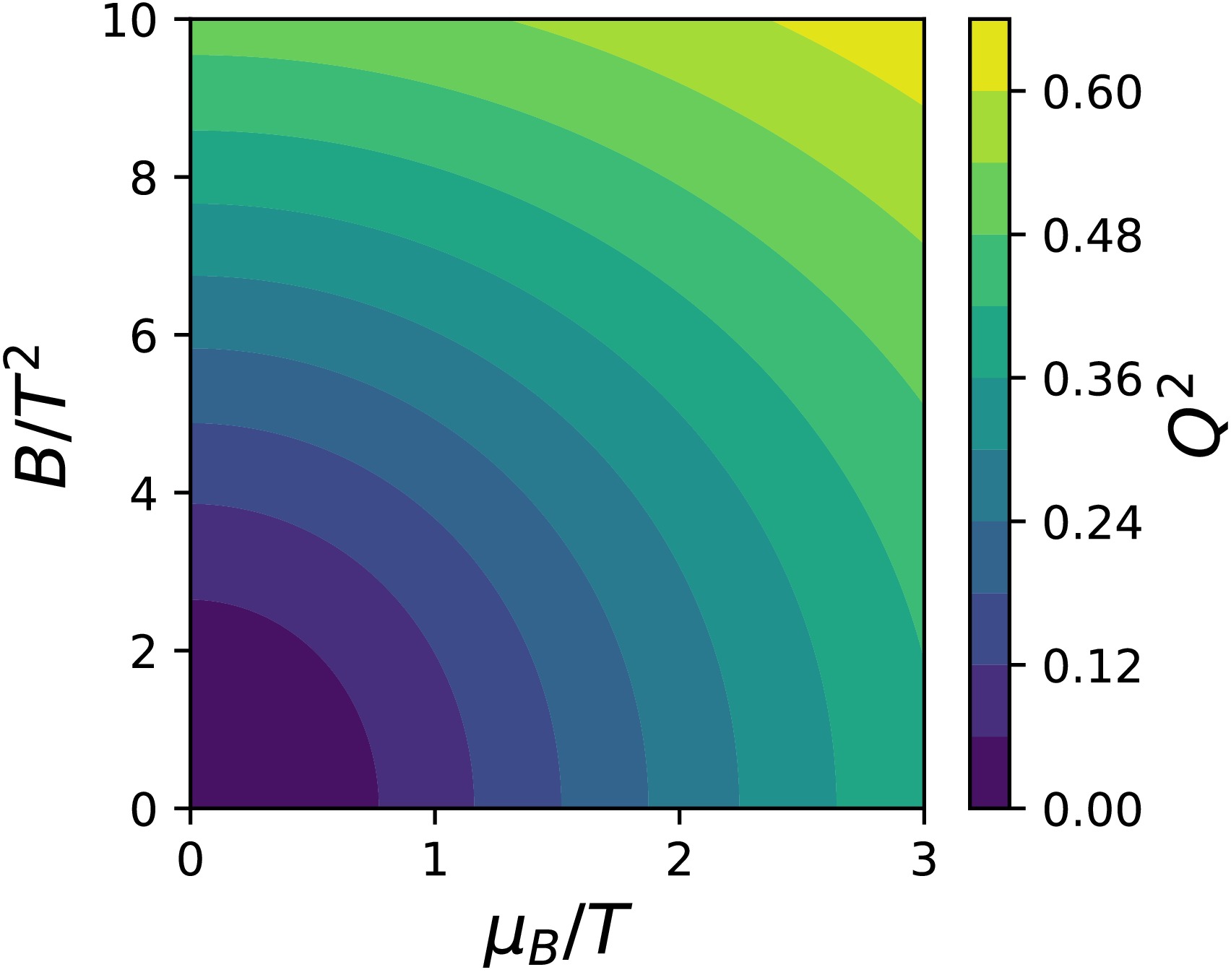
Figure 3. (color online) Squared effective charge
$ Q^2 $ as a function of the scaled baryon chemical potential and scaled magnetic field.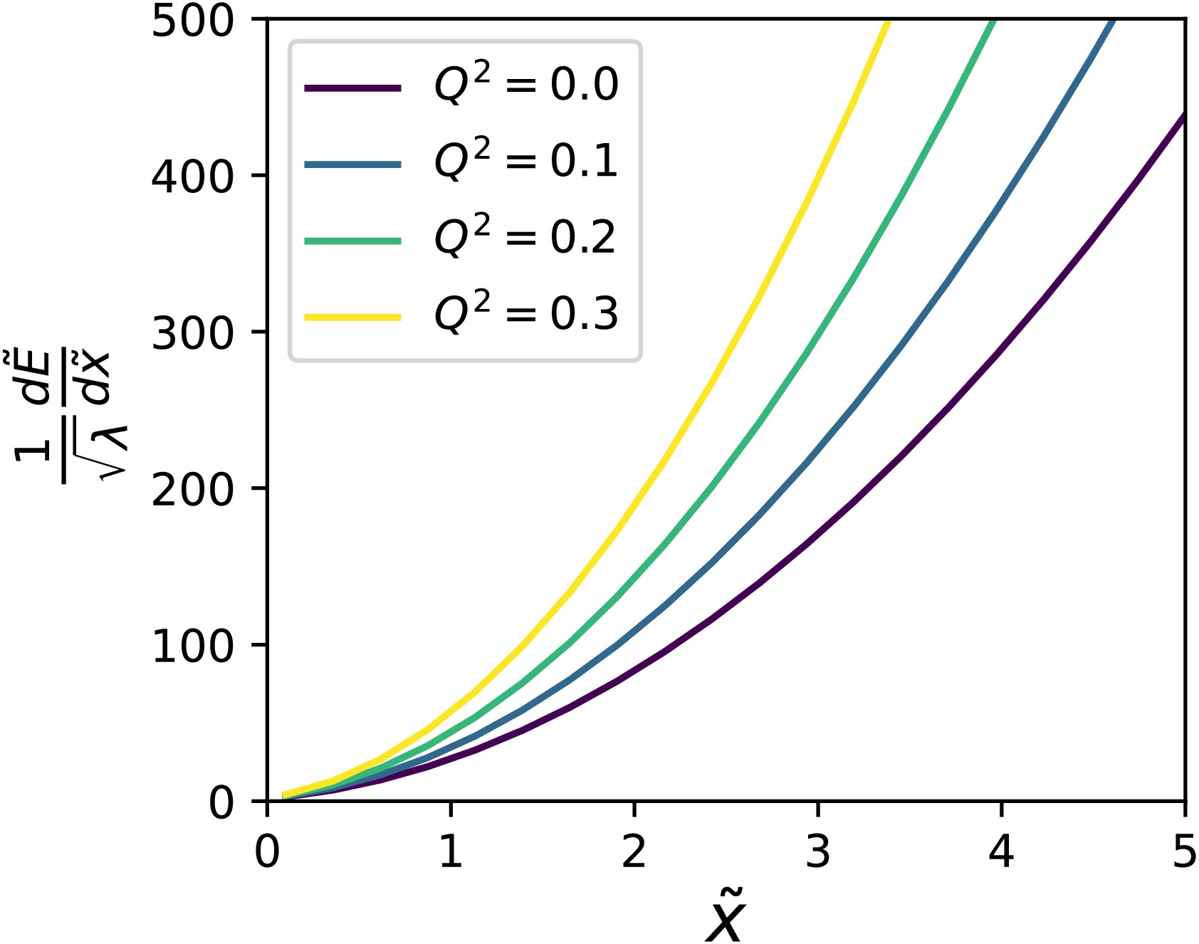
Figure 4. (color online) Rescaled energy loss as functions of the rescaled path length
$ \tilde{x} $ and external scale parameter$ Q^2 $ .If all external scale vanish
$ Q^2=0 $ , then the energy loss rate goes back to the formula used in Refs. [41, 42]$ \left.\frac{1}{\sqrt{\lambda}}\frac{{\rm d} \tilde{E}}{{\rm d}\tilde{x}}\right|_{\tilde{\mu}_B=0, \tilde{B}=0} = -\frac{\pi}{2} \left(\frac{1+\tilde{x}}{\tilde{z}_h(0,0)}\right)^2. $
(29) with
$ \tilde{z}_h(0,0)=1/\pi $ .In Fig. 5, we add the energy scales using different temperatures and perform unit conversion. Here, we measure energy loss rates in GeV/fm, path length in fm, temperature and chemical potential in GeV, and magnetic fields in
$ m_\pi^2 $ (setting the unit charge to one). In the upper panel of Fig. 5, we show the relationship between instantaneous energy loss rate$ \mathrm{d}E/\mathrm{d}x $ and distance x at different temperatures under the zero magnetic field and zero chemical potential. The results confirm that$ \mathrm{d}E/\mathrm{d}x $ increases with the temperature and path length. From Eq. (29), one can deduce that the limiting behavior at large$ \tilde{x}=xT $ is$ \mathrm{d}E/\mathrm{d}x\propto x^2T^4 $ , which is very different from those given by the perturbative calculations of collisional energy loss$ \mathrm{d}E_{\rm{c}oll}/\mathrm{d}x\propto g_s^4T^2 $ . In the lower panel of Fig. 5, we investigate the effects of the magnetic field and chemical potential on energy loss at a fixed temperature ($ T=0.2\;\mathrm{GeV} $ ). The calculations confirm that both the magnetic field and chemical potential enhance$ \mathrm{d}E/\mathrm{d}x $ , suggesting that they may be relevant for phenomenology at lower beam energies.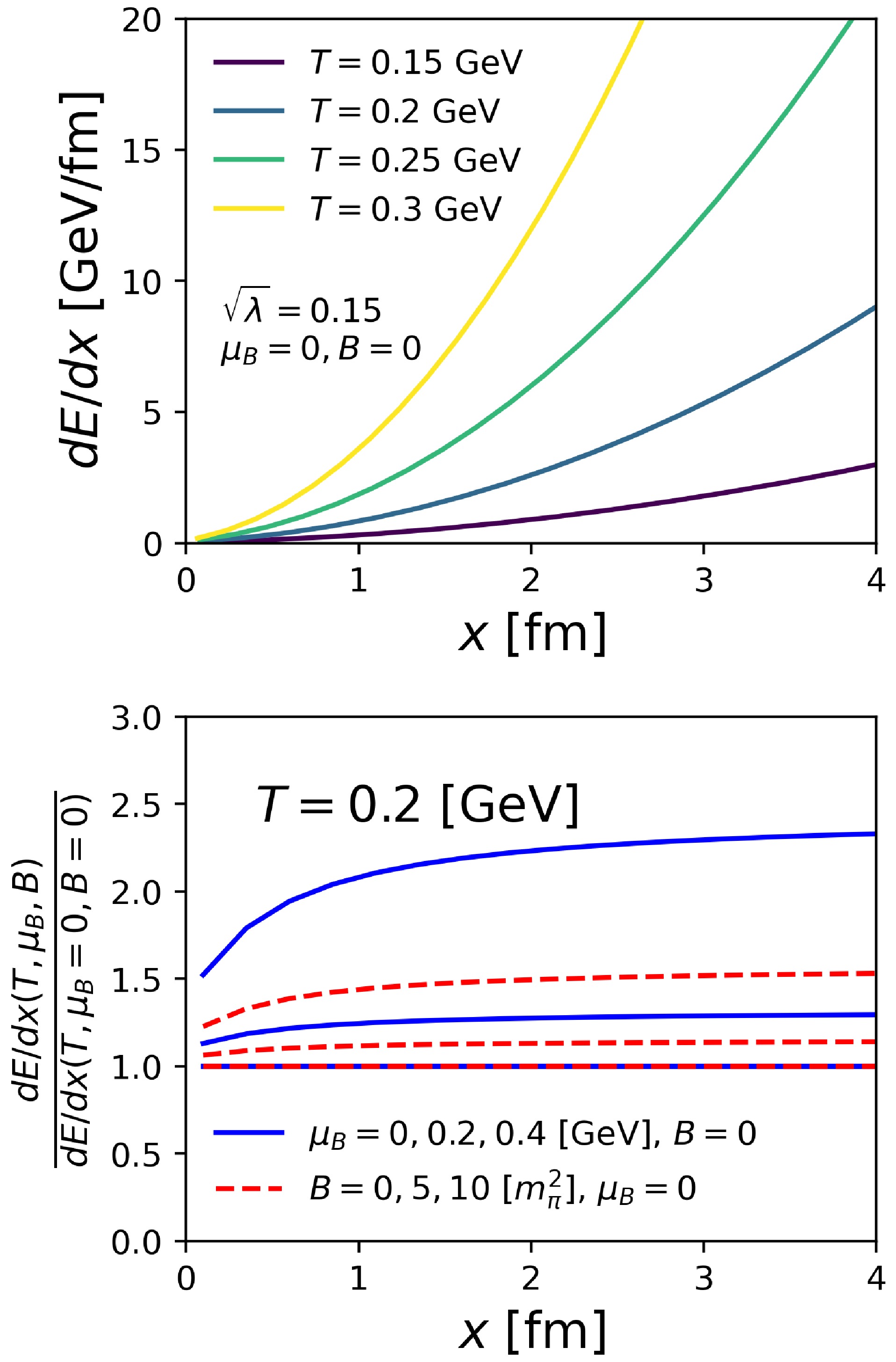
Figure 5. (color online) Upper panel: Physical energy loss per unit path length at different temperatures with the magnetic field and baryon chemical potential set to zero and
$ \sqrt{\lambda}=0.15 $ , respectively. Lower panel: Effects of the magnetic field and baryon chemical potential on energy loss at a fixed temperature of$ T = 0.2 $ GeV. -
We first set the magnetic field and chemical potential to zero, considering only the effect of λ on energy loss. The profile of temperature T is obtained from the ClVisc simulation of viscous relativistic hydrodynamics [88, 89]. We assume that λ is unchanged in a given center-of-mass energy. Under this assumption, λ can be considered an average value, recorded as
$ \langle\lambda\rangle $ . Then, we calculated the nuclear modification factor$ R_{AA} $ for central collisions in Au+Au at 200 GeV and Pb+Pb at 2.76 TeV and 5.02 TeV. Further, we use the$ \chi^{2}/d.o.f $ fitting of the calculated results against experimental data to extract the optimal value of$ \langle\lambda\rangle $ . The definition of$ \chi^{2}/d.o.f $ is$ \chi^{2}/d.o.f=\sum\limits_{i=1}^{N}\bigg[ \frac{(V^{\rm th}-V^{\rm exp})^{2}}{\sum\nolimits_{t}\sigma_{t}^{2}}\bigg]_{i}\bigg/N ,$
(30) where
$ V^{\mathrm{th}} $ represents the results obtained from theoretical calculations,$ V\mathrm{^{exp}} $ represents the experimental results,$ \sum\limits_{t}\sigma_{t}^{2} $ represents the sum of the squares of the different errors in the experimental data, and N represents the degree of freedom, which indicates the number of experimental data points. A smaller value of$ \chi^{2}/d.o.f $ indicates better agreement between the theoretical calculations and experimental data, while a larger value indicates worse agreement. The results confirm that the temperature of QGP rises with an increase in collision energy; thus,$ \langle\lambda\rangle $ decreases accordingly, as shown in Fig. 6. In our study, we incorporate a magnetic field and chemical potential within the AdS/CFT duality framework as a model for investigating the jet quenching effect. Although the final numerical value of λ is very small, we focus on examining the dependence of jet quenching on the magnetic field and chemical potential within the model framework. The apparent inconsistency suggests that jet quenching may not be entirely governed by strong-coupling dynamics but could also involve perturbative processes such as radiation. The primary objective of our study is to utilize this model for exploring the dependence of energy loss on the magnetic field and chemical potential.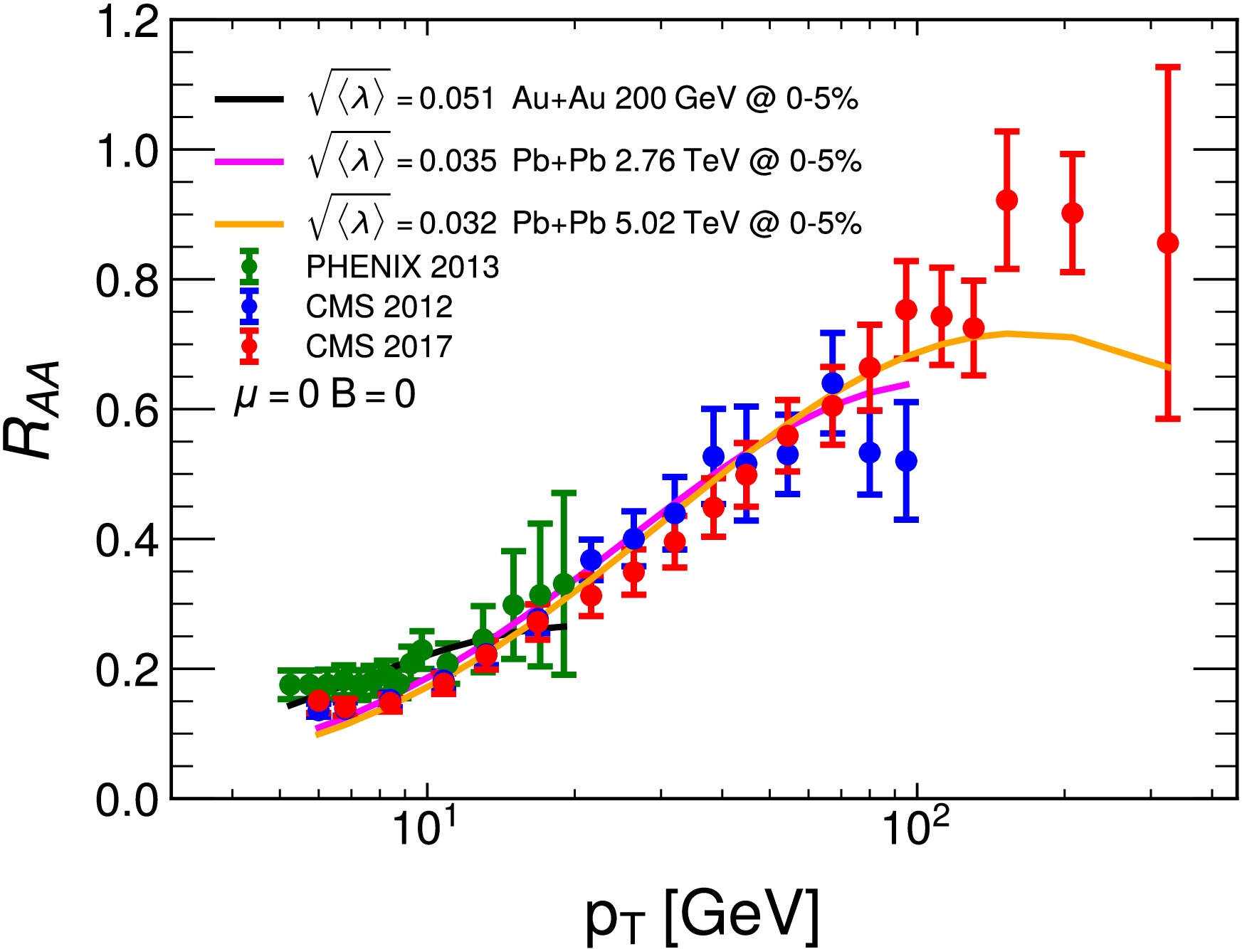
In Ref. [93], the results showed that
$ \hat{q}/T^{3} $ decreases with local temperature T for a jet propagating through the QGP medium, as indicated in the upper panel of Fig. 7. This result is consistent with the trend of the mass-center energy dependence of$ \langle\lambda\rangle $ calculated above in Fig. 6, as shown in the lower panel of Fig. 7, where$ \sqrt{\langle\lambda\rangle} $ decreases with increasing center-of-mass energy. Considering the medium temperature increases with the collision energy, we assume that the temperature dependence of$ \sqrt{\langle\lambda\rangle} $ is proportional to the temperature dependence of$ \hat{q}/T^{3} $ ; therefore, in the later part of the paper, we adopt the temperature-dependent 't Hooft coupling$ \lambda(T) $ .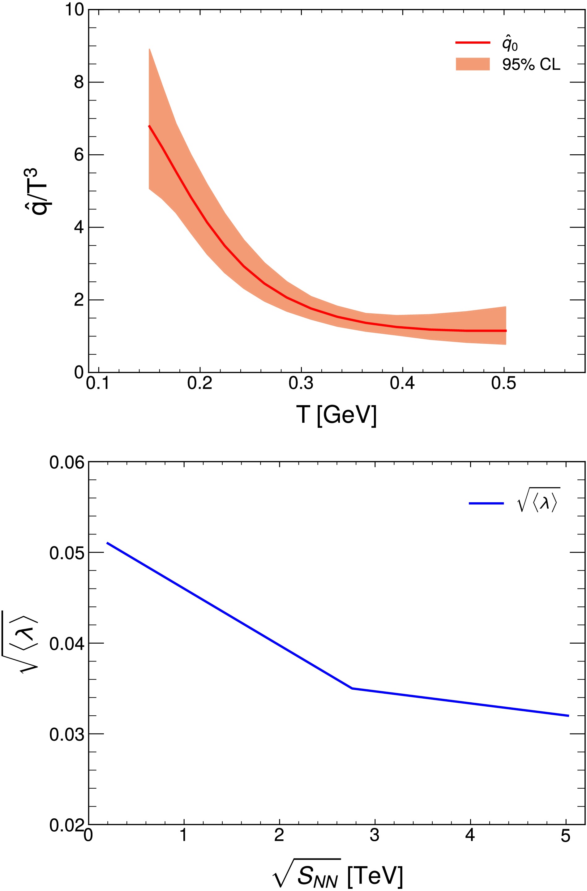
Figure 7. (color online) Upper panel: Dependence of
$ \hat{q}/T^{3} $ on temperature [93]. Lower panel: Dependence of$ \sqrt{\langle\lambda\rangle} $ on the center-of-mass energy.In a hot
$ {\cal{N}}=4 $ SYM theory, a relationship between$ \hat{q}/T^{3} $ and$ \sqrt{\lambda} $ is obtained [20] as$ \hat{q}_{\mathrm{SYM}}\sim\sqrt{\lambda}T^{3}. $
(31) Therefore, we will parametrize the temperature dependence of the 't Hooft coupling by relating it to the temperature dependence of
$ \hat{q}/T^{3} $ .$ \lambda(T)=\big(\hat{q}/T^{3}\big)\big/c, $
(32) where
$ \hat{q}/T^{3} $ as a function of T is given by Ref. [93], and c represents a tunable constant to be fixed by experiments. Therefore, Eq. ($ 32 $ ) is the temperature-dependent$ \lambda(T) $ . To determine c, we consider that, for central nucleus-nucleus collisions at LHC energies such as central Pb+Pb collisions at 2.76 or 5.02 TeV, the effect of the magnetic field and chemical potential are both negligible, i.e.,$ B \to 0 $ and$ \mu_{B} \to 0 $ [58]. With the jet energy loss obtained by substituting Eq. ($ 32 $ ) in Eq. ($ 24 $ ), we calculate the nuclear modification factor$ R_{AA} $ for the central Pb+Pb collisions at 2.76 TeV (according to Ref. [93]. The calculation results for Pb+Pb 2.76 TeV match the experimental data best, and we utilize the result from the$ \hat{q}_{0} $ line in the upper panel of Fig. 7. Then, we performed a$ \chi^{2}/d.o.f $ fitting of the calculated results against the experimental data for extracting the best-fitting constant c. Figure 8 shows the values of$ \chi^{2}/d.o.f $ corresponding to the different values of constant c. Figure 8 shows that, when c = 105, the agreement with the experimental data is the best. Therefore, in the following calculations, the value of constant c in Eq. ($ 32 $ ) is fixed at 105.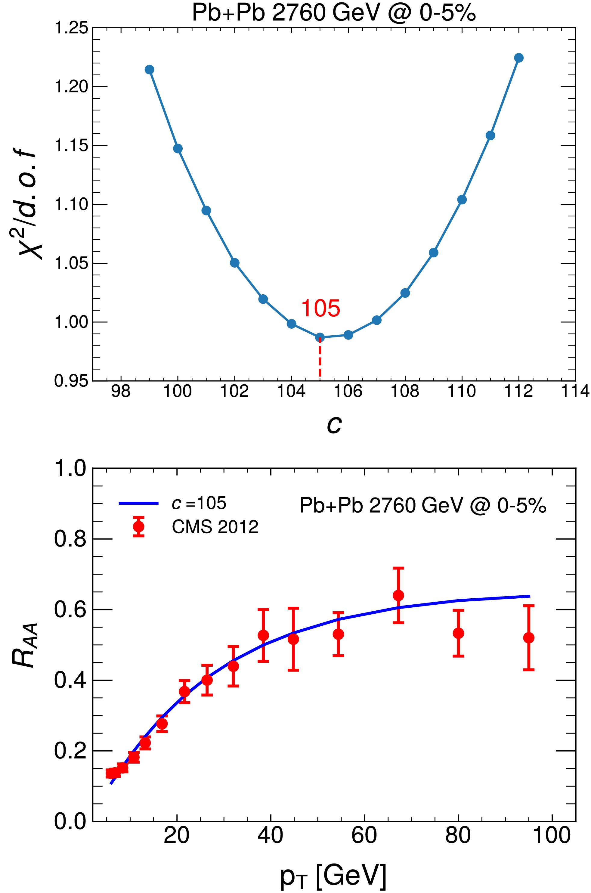
Figure 8. (color online) Upper panel:
$ \chi^{2}/d.o.f $ fitting for the proportionality coefficient c with the nuclear modification in 0−5% Pb+Pb collisions at$ \sqrt{s_{NN}}=2.76 $ TeV. Lower panel: Comparison between the nuclear modification factor$ R_{AA} $ calculated with the best-fitting value$ c=105 $ and the data [66]. -
Using this temperature-dependent coupling, we illustrate the effect of
$ \mu_{B} $ and B in the total energy loss. We calculate the energy loss as a function of τ for a quark jet that is initially produced at the center of the QGP ($ x=y=z=0 $ ) and propagates in the transverse direction ($ \eta = 0 $ ) along direction$ \phi = 0 $ through the QGP. The energy loss at τ is the integral of the energy loss rate from$ \tau_0 $ to τ,$ \Delta E(\tau)=\int_{\tau_0}^{\tau}\mathrm{d}x\mathrm{d}E/\mathrm{d}x $ . Figure 9 shows the average energy loss dependent on the magnetic field and the chemical potential in 10%−20% Au+Au collisions at$ \sqrt{s_{NN}}=200 $ GeV and 10%−30% Pb+Pb collisions at$ \sqrt{s_{NN}}=2.76, 5.02 $ TeV, respectively.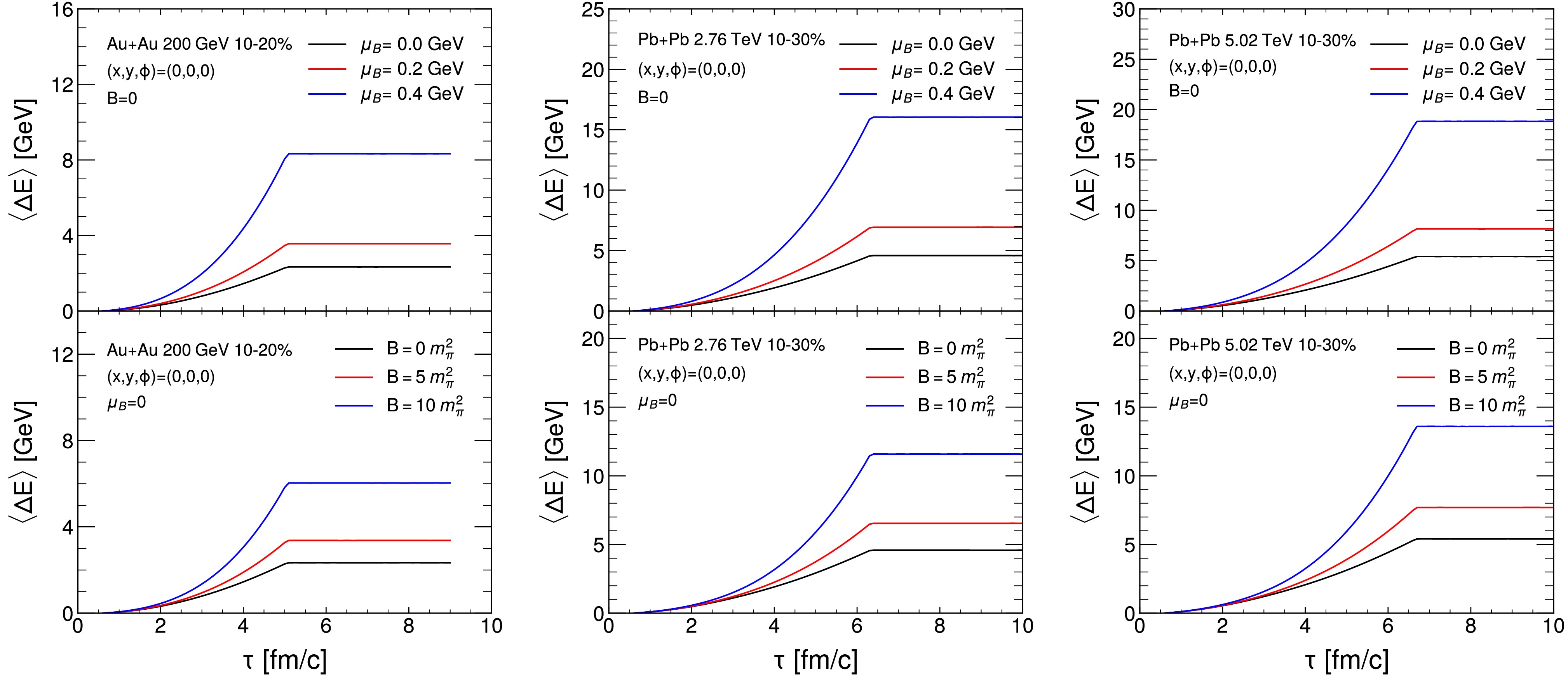
Figure 9. (color online) Average energy loss dependent on the magnetic field and chemical potential in 10%−20% Au+Au collisions at
$ \sqrt{s_{NN}}=200 $ GeV and 10%−30% Pb+Pb collisions at$ \sqrt{s_{NN}}=2.76, 5.02 $ TeV, respectively. Upper panels: Effect of the chemical potential on the average energy loss of jet. Lower panels: Effect of the magnetic field on the average energy loss of the jet.In principle, the time evolution of the magnetic field and baryon chemical potential should be obtained from a dynamical model, e.g., magneto-hydrodynamic equations with conserved charge and the corresponding equation of state. However, these tools are not yet sophisticated for the jet quenching study. Therefore, in this study, we considered a very simplistic approach to treat B and
$ \mu_B $ as background fields and parametrized their time dependence in two extreme cases.$ \text{Scenario I}: \quad \mu_B = \text{const}, \quad B= \text{const}. $
(33) $ \text{Scenario II}: \quad \frac{\mu_B}{T} = \text{const}, \quad \frac{B}{T^2}= \text{const}. $
(34) The
$ \mu_B/T $ trajectories of the two cases are illustrated in the phase diagram shown in Fig. 10. Although these are clearly not the physical case, we hope by tuning the constants in each scenario that it can mimic the physical trajectory from hydrodynamic simulations with a finite baryon chemical potential. For the magnetic field, scenario II parametrizes a field that decays over time. In Fig. 9, we plot the energy loss with fields turned on in the first scenario. In the upper panel, we set B to 0, and$ \mu_{B} $ takes the values from 0 to 0.4 GeV. Similarly, we set$ \mu_{B} $ to 0 in the bottom panel, and B takes the values from 0 to 10$ m_{\pi}^2 $ . The energy loss increases monotonically with$ \mu_{B} $ and B, which is consistent with Refs. [44, 59, 60].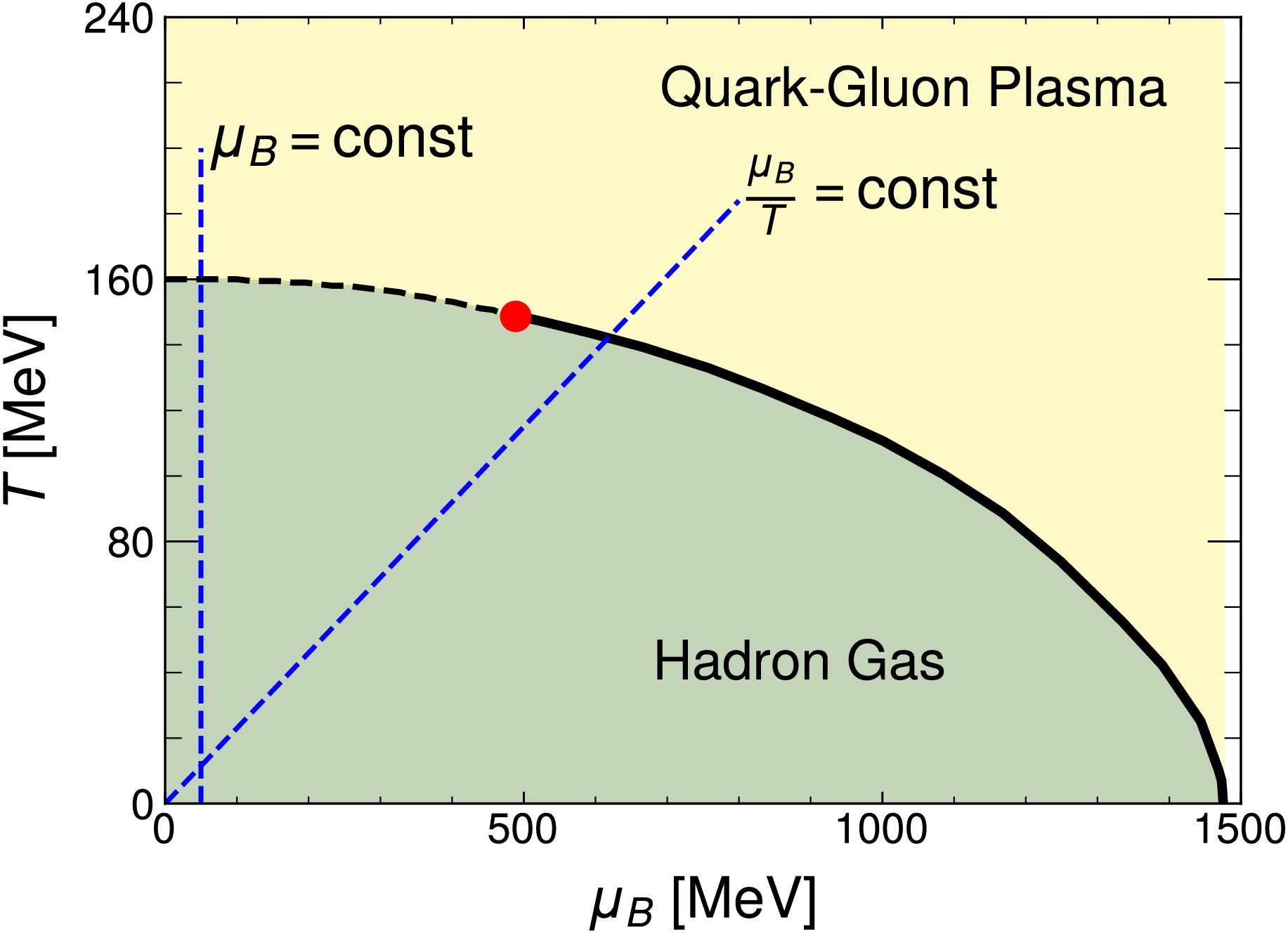
Figure 10. (color online) Trajectory of a jet in the phase diagram under the conditions of constant
$ \mu_{B} $ and constant$ \mu_{B}/T $ . -
The method of Bayesian inference for the model parameters has achieved significant success in the field of relativistic heavy-ion collisions [94−96]. For example, the shear viscosity
$ \eta/s $ of the QGP medium [97, 98], jet transport coefficient$ \hat{q} $ [62, 93, 99], and analysis of the jet energy loss [100, 101]. In this study, we utilize the Bayesian inference method to constrain the magnetic field and chemical potential in the energy loss functions of partons traversing the QGP medium, obtaining the variation in the magnetic field and chemical potential in heavy-ion collisions. The Bayesian analysis process is illustrated in Fig. 11.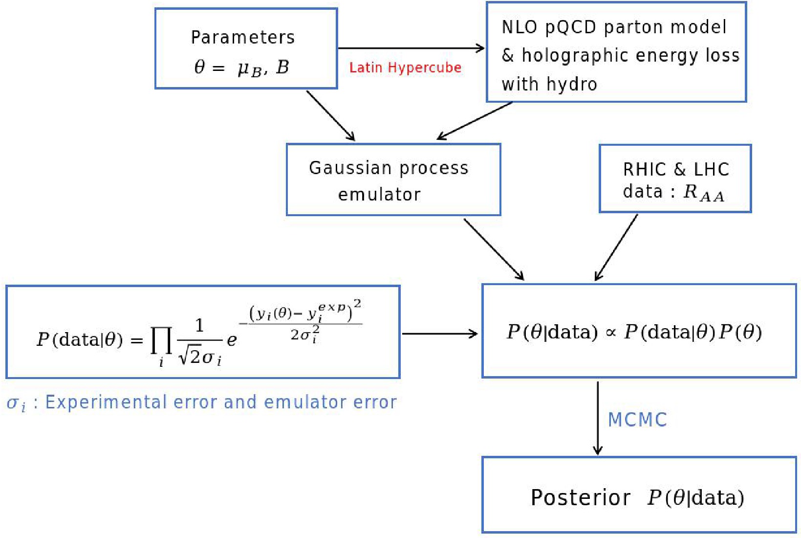
Figure 11. (color online) Flowchart of the Bayesian analysis.
The set of parameters is denoted by θ. Based on Bayes' theorem,
$ \mathit{P}(\theta| \mathrm{data})=\frac{\mathit{P}(\mathrm{data}|\theta)\mathit{P}(\theta)}{P(\mathrm{data})} .$
(35) $ \mathit{P}(\theta| \mathrm{data}) $ represents the posterior distribution, which is the conditional probability of parameters given the observed data.$ \mathit{P}(\theta) $ represents the prior distribution, which reflects our initial assumptions or knowledge about the parameters.$ \mathit{P}(\mathrm{data} |\theta) $ refers to the likelihood or probability of observing the data based on specific assumed parameter values. In our work,$ \boldsymbol{\theta}=(\mu_{B}, B) $ is a two-dimensional vector and$ \mathit{P}(\mathrm{data}|\theta) $ is assumed to follow a Gaussian distribution.$ \mathit{P}(\mathrm{data}|\theta)=\frac{1}{(2\pi)^{N/2}|\Sigma|^{1/2}}\mathrm{e}^{-\frac{1}{2}[\boldsymbol{y}(\theta)-\boldsymbol{y}^{\text{exp}}]^T\Sigma^{-1}[\boldsymbol{y}(\theta)-\boldsymbol{y}^{\text{exp}}]} .$
(36) Here,
$ \boldsymbol{y}^{\text{exp}} $ represents the vectorized$ R_{AA} $ experimental data. Further,$ \boldsymbol{y}(\theta) $ represents the theoretical$ R_{AA} $ values computed across various centralities at both RHIC and LHC, including Au+Au collisions at$ \sqrt{s_{NN}} = 200\ \mathrm{GeV} $ (10%−20%, 20%−30%, and 40%−50% centralities) and Pb+Pb collisions at$ \sqrt{s_{NN}} = 2.76\ \mathrm{TeV} $ and$ 5.02\ \mathrm{TeV} $ (10%−30%, 30%−50%, and 50%−70% centralities). This model evaluation is surrogated by a Gaussian emulator [102, 103] trained using 300 sets of input parameters with full-model calculations. Σ represents the covariance matrix that have included both experimental uncertainty and Gaussian emulator uncertainty. The experimental uncertainties include both systematic and statistical errors.In our following calculations, we set two cases of constant magnetic field and chemical potential, as shown in Fig. 10. We assume that both the magnetic field and chemical potential remain constant throughout the entire heavy-ion collision process. We also assume that dimensionless observables remain constant during the collision process, which are the ratio of the magnetic field over temperature T squared and ratio of the chemical potential over temperature T. Given the complexity of the jet behavior as it moves through the medium in heavy-ion collisions. Further, a self-consistent theoretical framework that can describe the coupled evolution of magnetic fields, chemical potential, and QGP medium remains underdeveloped. Conducting such comprehensive dynamic coupling simulations would be computationally prohibitive. Therefore, our approach employs two simplified scenario assumptions to preliminarily investigate the effects of magnetic fields and chemical potential on jet quenching, as well as their behaviors across different collision energies and centrality classes. Starting from the prior, we set a uniform prior distribution
$ \mu_{B}\in $ (0, 0.3)$ \mathrm{GeV} $ and$ B\in $ (0, 15)$ m_{\pi}^{2} $ in the first assumption, and$ \mu_{B}/T\in $ (0, 3) and$ B/T^{2}\in $ (0, 10) in the second assumption. Within this prior range, we use Latin hypercube sampling to obtain 300 design points. These 300 sets of parameters were input into the$ \mathrm{NLO} $ $ \mathrm{pQCD} $ parton model for calculating the nuclear modification factor$ R_{AA} $ for hadrons in different-centrality Au+Au collisions at 200 GeV and in different-centrality Pb+Pb collisions at 2.76 or 5.02 TeV. Subsequently, we trained these 300 design points and their corresponding model outputs into a Gaussian emulator for use in subsequent Bayesian inference.We use Markov chain Monte Carlo (MCMC) [104, 105] for Bayesian calibration. MCMC is based on the Metropolis-Hastings (M-H) algorithm for sampling posterior probabilities. This algorithm generates samples by performing a random walk in the parameter space and accepting or rejecting each step based on posterior probability to extract the probability distribution of parameter space θ. In our MCMC sampling, we utilized 60 walkers and performed a total of 20000 sampling steps. The first 10000 steps were discarded as burn-in, while the remaining 10000 steps were used to obtain a well-converged posterior distribution.
-
Based on the Bayesian inference framework, we extract the distributions of magnetic field and chemical potential from the nuclear modification factor
$ R_{AA} $ of the data [66, 67, 92] for hadron production across different-centrality collision systems and different collision energies. These data are for 10%−20%, 20%−30%, and 40%−50% Au+Au collisions at$ \sqrt{s_{NN}}=200 $ GeV, and 10%−30%, 30%−50%, and 50%−70% Pb+Pb collisions at$ \sqrt{s_{NN}}=2.76 $ or 5.02 TeV, respectively. We begin with the constant magnetic field and chemical potential, and then with the scaled magnetic field and chemical potential.As shown in Fig. 12, the Bayesian inference of the magnetic field and chemical potential (diagonal panels) and their correlations (off-diagonal panels) in different-centrality A+A collisions at 0.2, 2.76, and 5.02 TeV. These figures present the posterior probability distributions of the magnetic field and chemical potential obtained by fitting experimental data for nuclear modification factors. The diagonal panels show marginal distributions of the magnetic field and chemical potential (Red dashed line indicates the position of the median) with 95% confidence levels (CL), whereas the off-diagonal panels display their joint distributions. The left column corresponds to
$ \sqrt{s_{NN}} $ = 200 GeV with centralities of 10%−20%, 20%−30%, and 40%−50% in Au-Au collisions; the middle column corresponds to$ \sqrt{s_{NN}} $ = 2.76 TeV with centralities of 10%−30%, 30%−50%, and 50%−70% in Pb-Pb collisions; and the right column corresponds to$ \sqrt{s_{NN}} $ = 5.02 TeV with the same centralities in the Pb-Pb collisions.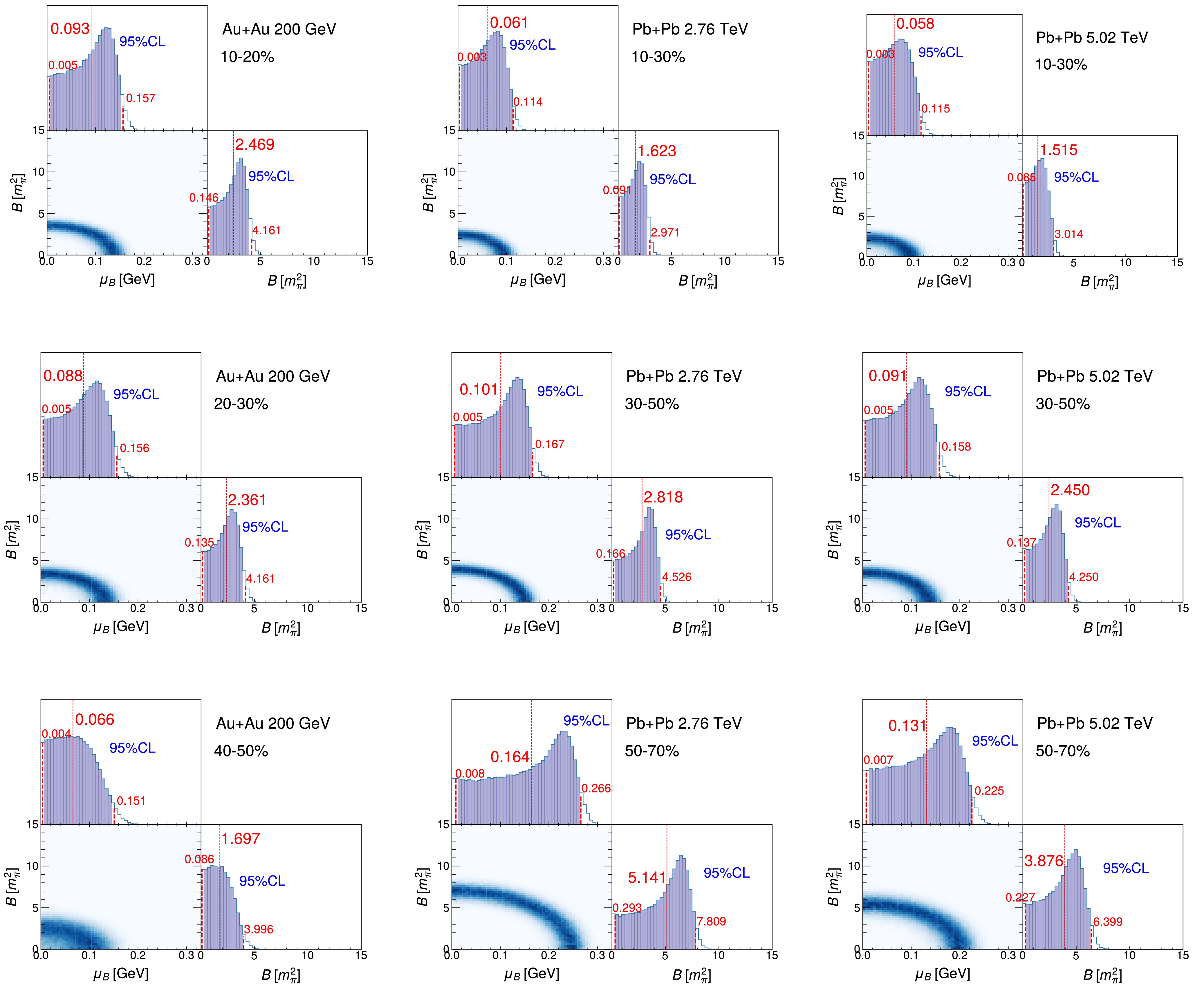
Figure 12. (color online) Bayesian inference of the magnetic field and chemical potential (diagonal panels) and their correlations (off-diagonal panels). Left column: For 10%−20%, 20%−30%, and 40%−50% Au+Au collisions at
$ \sqrt{s_{NN}} $ = 200 GeV. Center column: For 10%−30%, 30%−50%, and 50%−70% Pb+Pb collisions at$ \sqrt{s_{NN}} $ = 2.76 TeV. Right column: For 10%−30%, 30%−50%, and 50%−70% Pb+Pb collisions at$ \sqrt{s_{NN}} $ = 5.02 TeV. The data are from PHENIX and CMS on the charged-hadron$ R_{AA} $ [66, 67, 92].The results indicate good alignment between the parameters of the magnetic field and chemical potential with experimental data. A distinct negative correlation is observable between the magnetic field and chemical potential. This correlation stems from the fact that both parameters augment jet energy loss in the same direction, which indicates that an increase in one can be counterbalanced by a decrease in the other to uphold consistency. Further investigation shows that, at a constant collision centrality, the chemical potential diminishes as the collision energy escalates, which is in accordance with the findings in Ref. [58]. Given the negative correlation between the chemical potential and magnetic field, the magnetic field diminishes with an increase in collision energy, aligning with the conclusion of Ref. [47]. At a fixed collision energy, both the magnetic field and chemical potential intensify as the collision geometry becomes more eccentric (i.e., centrality rises).
$ \mu_{B} $ and B obtained under the constant assumption represent an overall effect. However, the magnetic field strength decays rapidly at the early stage, and then, it decays inversely proportional to the time once the QGP is formed and responds to the electromagnetic field [47]. Thus, one can assume that$ \mu_{B} $ and B follow the same pattern of time evolution as T. Figure 13 shows the scaled magnetic fields ($ B/T^2 $ ) and scaled chemical potentials ($ \mu_{B}/T $ ). The calculation methodology is similar to that in Fig. 12. The results indicate that, at the same collision centrality, the scaled magnetic field and scaled chemical potential decrease with an increase in the collision energy. Conversely, at the same collision energy, both the scaled magnetic field and scaled chemical potential exhibit a rising trend as the degree of collision eccentricity rises (i.e., as centrality increases). These findings provide further insights into the systematic behavior of the magnetic field and chemical potential in high-energy nuclear collisions. In Au+Au collisions, the experimental ranges of the ratio of chemical freeze-out temperature to baryon chemical potential are provided for the centralities of 10%−20%, 20%−30% and 40%−60%. The red rectangular shaded region represents results obtained using the GCEY method, while the blue rectangular shaded region represents results obtained using the GCER method. Both methods are sourced from Ref. [106]. Since the experimental literature does not provide data for 40%−50% centrality, we use the experimental results for 40%−60% centrality as an approximation and compare them with our calculated results for 40%−50% centrality. However, in Pb+Pb collisions at LHC, the ratio of chemical freeze-out temperature to baryon chemical potential approaches zero [107], as indicated by the red rectangular shaded region.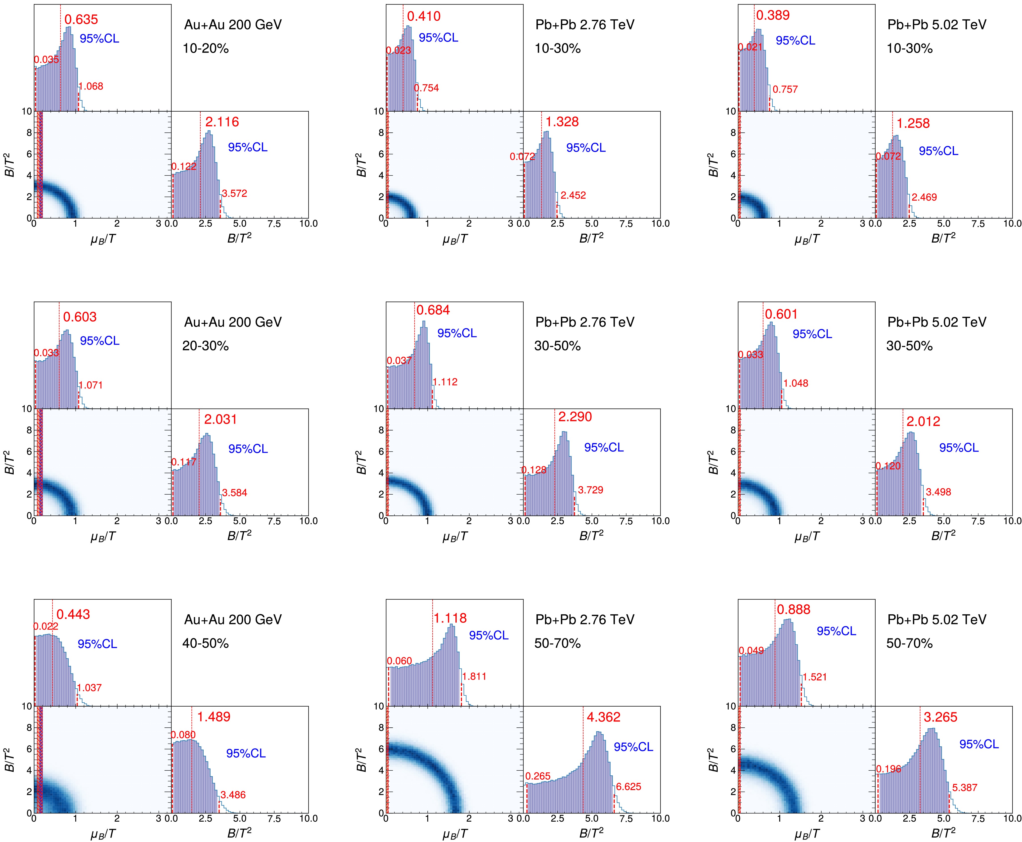
Figure 13. (color online) The posterior distributions of the scaled magnetic field and scaled chemical potential (diagonal panels) and their correlations (off-diagonal panels). Left column: 10%−20%, 20%−30%, and 40%−50% Au+Au collisions at
$ \sqrt{s_{NN}} $ = 200 GeV. Center column: 10%−30%, 30%−50%, and 50%−70% Pb+Pb collisions at$ \sqrt{s_{NN}} $ = 2.76 TeV. Right column: 10%−30%, 30%−50%, and 50%−70% Pb+Pb collisions at$ \sqrt{s_{NN}} $ = 5.02 TeV. Wth experimental data sourced from PHENIX and CMS on the$ R_{AA} $ of charged light hadrons [66, 67, 92]. In Au+Au collisions, the red and blue rectangular shaded regions correspond to the experimental ranges of the chemical freeze-out temperature to baryon chemical potential ratio for the 10%−20%, 20%−30%, and 40%−60% centrality, respectively [106]. Since experimental data are not available for the 40%−50% centrality, we compare our 40%−50% centrality results with the experimental results from the 40-60% centrality in our calculations. In Pb+Pb collisions at LHC, the ratio of chemical freeze-out temperature to baryon chemical potential approaches nearly zero [107], as indicated by the red rectangular shaded region.Using the above extraction values for the magnetic field, chemical potential, scaled magnetic field, and scaled chemical potential, we present the prior and posterior nuclear modification factors
$ R_{AA} $ in the Appendix, compared with data in different-centrality A+A collisions at 0.2, 2.76, and 5.02 TeV, respectively. Our posterior results fit the data well. -
In relativistic heavy-ion collisions, the jet quenching effect is an important phenomenon that provides a unique experimental window for studying the microscopic properties and dynamical behavior of the QGP. Jet quenching describes the energy loss of high energy jets as they traverse the QGP, which can be attributed to strong interactions with the medium. This effect can be indirectly observed through the experimentally measured transverse momentum nuclear modification factor
$ R_{AA} $ . However, the specific effect of the magnetic field and chemical potential in the QGP medium on the jet energy loss has not yet been thoroughly investigated. Inspired by this scientific question, we derived a jet energy loss formula incorporating the effects of the magnetic field and chemical potential based on the AdS/CFT correspondence, which describes the energy attenuation of partons moving through the QGP medium. We employed Bayesian inference to systematically compare the theoretical predictions with the experimentally measured$ R_{AA} $ data to validate the applicability of the theoretical model and reveal the effect of the magnetic field and chemical potential on jet quenching. Using this approach, we simultaneously extracted, for the first time, the distributions of the magnetic field and chemical potential in the QGP under different collision energies and centrality.Our findings reveal the following key patterns: (i) Enhancement of jet energy loss by the magnetic field and chemical potential: The presence of the magnetic field and chemical potential significantly enhances the jet energy loss effect, which indicates that these properties of the QGP medium play a crucial role in the strong interactions between partons and the medium. (ii) Impact of collision centrality: As the collisions tend to become more eccentric, the strengths of the magnetic field and chemical potential increase significantly. This reflects the more pronounced local charge asymmetry generated in the collisions. (iii) Impact of collision energy: With increasing collision energy, both the magnetic field and chemical potential exhibit a decreasing trend. This phenomenon may be related to the expansiveness of the QGP and changes in initial conditions at higher energies. (iv) Theoretical calculations show that magnetic field and chemical potential affects the energy loss in a highly correlated manner: Extracting only the energy loss rate cannot provide a unique sensitivy to only one of the two effects. Within the current theoretical framework, the physical mechanism by which magnetic fields enhance energy loss can be attributed to two aspects. Magnetic fields reduce the viscosity of the QGP medium [59], intensifying strong interactions among partons and leading to greater energy loss. Magnetic fields may lower the critical temperature of the QCD phase transition [57], extending the temperature range over which the medium remains in a strongly coupled state, further amplifying energy dissipation.
These research findings not only enrich our theoretical understanding of the effects of the magnetic field and chemical potential on jet energy loss but also provide a new direction for experimentally exploring the physical properties of the QGP using
$ R_{AA} $ data. -
We extend our gratitude to Prof. Defu Hou and Dr. Zhou-Run Zhu for the assistance and valuable suggestions provided.
-
We extend our gratitude to Prof. Defu Hou and Dr. Zhou-Run Zhu for the assistance and valuable suggestions provided.
-
We extend our gratitude to Prof. Defu Hou and Dr. Zhou-Run Zhu for the assistance and valuable suggestions provided.
-
The calculation procedure for the nuclear modification factor
$ R_{AA} $ is as follows: We employ the CLVisc hydrodynamic framework [88, 89] to provide the temperature parameter T for the holographic energy loss model, which fully describes the thermodynamic evolution of the medium in heavy-ion collisions. By integrating the holographic energy loss model with CLVisc, we construct a systematic energy loss table that records the total energy loss accumulated by partons as they traverse the QGP medium from various initial positions and directions. This energy loss table is then incorporated into Eq. (2) of the main text to compute the final-state inclusive hadron yield in nucleus-nucleus collisions. For the inclusive hadron production cross-section in proton-proton collisions, we calculated it using Eq. (1) of the main text, with the results shown in Fig. 1. Finally, following the definition of$ R_{AA} $ in Eq. (6), we divide the nucleus-nucleus collision yield by the proton-proton collision cross-section to obtain the numerical value of$ R_{AA} $ .Figure A1 (based on the first assumption) and Fig. A2 (based on the second assumption) present the calculated nuclear modification factor
$ R_{AA} $ in comparison with the experimental data. These two figures illustrate the computational results of the model under different assumptions. In these figures, the top panels show the prior results, reflecting the initial predictive capability of the model without fully utilizing experimental information. The bottom panels display the posterior results obtained through Bayesian inference. The posterior results achieve significantly better agreement with the experimental data, demonstrating the optimization of the model after incorporating experimental inputs. This not only validates the feasibility of the modeling method but also enhances its capability and reliability in describing the actual physical processes. These findings are of great significance for gaining deeper insights into related phenomena.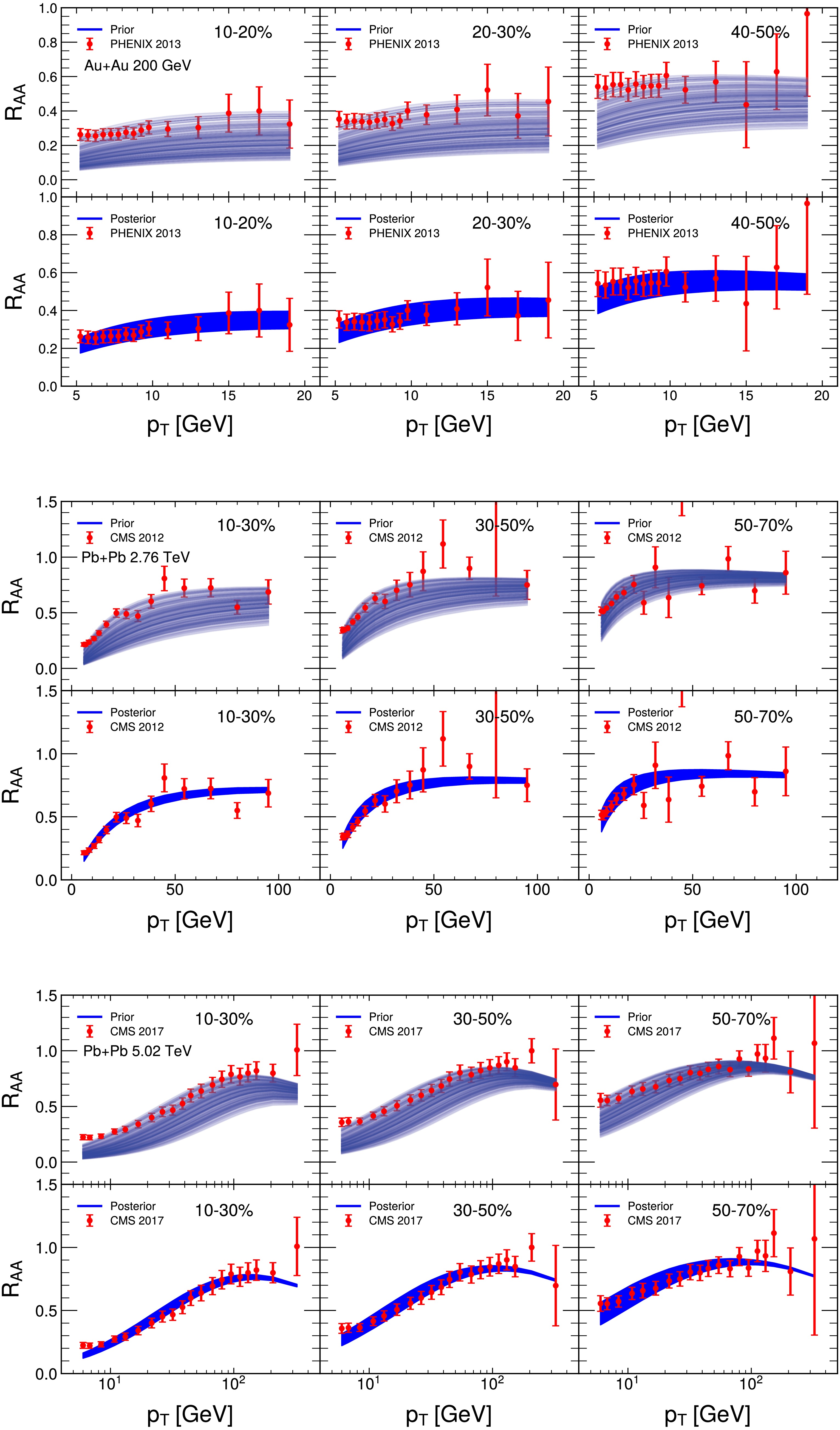
Figure A1. (color online) Calibration of the NLO pQCD model calculations against the
$ R_{AA} $ data of charged light hadrons from PHENIX and CMS [66, 67, 92]. Upper line: 10%−20%, 20%−30%, and 40%−50% Au+Au collisions at$ \sqrt{s_{NN}} $ = 200 GeV. Center line: 10%−30%, 30%−50%, and 50%−70% Pb+Pb collisions at$ \sqrt{s_{NN}} $ = 2.76 TeV. Lower line: 10%−30%, 30%−50%, and 50%−70% Pb+Pb collisions at$ \sqrt{s_{NN}} $ = 5.02 TeV. The upper panel shows the calculations performed using the prior distributions of the magnetic field and chemical potential, while the lower panel displays the posterior distributions after calibration.
Figure A2. (color online) Calibration of the NLO pQCD model calculations against the
$ R_{AA} $ data of charged light hadrons from PHENIX and CMS [66, 67, 92]. Upper line : 10%−20%, 20%−30%, and 40%−50% Au+Au collisions at$ \sqrt{s_{NN}} $ = 200 GeV. Center line: 10%−30%, 30%−50%, and 50%−70% Pb+Pb collisions at$ \sqrt{s_{NN}} $ = 2.76 TeV. Lower line: 10%−30%, 30%−50%, and 50%−70% Pb+Pb collisions at$ \sqrt{s_{NN}} $ = 5.02 TeV. The upper panel shows the calculations performed using the prior distributions of the scaled magnetic field and scaled chemical potential, while the lower panel displays the posterior distributions after Bayes inference. -
The calculation procedure for the nuclear modification factor
$ R_{AA} $ is as follows: We employ the CLVisc hydrodynamic framework [88, 89] to provide the temperature parameter T for the holographic energy loss model, which fully describes the thermodynamic evolution of the medium in heavy-ion collisions. By integrating the holographic energy loss model with CLVisc, we construct a systematic energy loss table that records the total energy loss accumulated by partons as they traverse the QGP medium from various initial positions and directions. This energy loss table is then incorporated into Eq. (2) of the main text to compute the final-state inclusive hadron yield in nucleus-nucleus collisions. For the inclusive hadron production cross-section in proton-proton collisions, we calculated it using Eq. (1) of the main text, with the results shown in Fig. 1. Finally, following the definition of$ R_{AA} $ in Eq. (6), we divide the nucleus-nucleus collision yield by the proton-proton collision cross-section to obtain the numerical value of$ R_{AA} $ .Figure A1 (based on the first assumption) and Fig. A2 (based on the second assumption) present the calculated nuclear modification factor
$ R_{AA} $ in comparison with the experimental data. These two figures illustrate the computational results of the model under different assumptions. In these figures, the top panels show the prior results, reflecting the initial predictive capability of the model without fully utilizing experimental information. The bottom panels display the posterior results obtained through Bayesian inference. The posterior results achieve significantly better agreement with the experimental data, demonstrating the optimization of the model after incorporating experimental inputs. This not only validates the feasibility of the modeling method but also enhances its capability and reliability in describing the actual physical processes. These findings are of great significance for gaining deeper insights into related phenomena.
Figure A1. (color online) Calibration of the NLO pQCD model calculations against the
$ R_{AA} $ data of charged light hadrons from PHENIX and CMS [66, 67, 92]. Upper line: 10%−20%, 20%−30%, and 40%−50% Au+Au collisions at$ \sqrt{s_{NN}} $ = 200 GeV. Center line: 10%−30%, 30%−50%, and 50%−70% Pb+Pb collisions at$ \sqrt{s_{NN}} $ = 2.76 TeV. Lower line: 10%−30%, 30%−50%, and 50%−70% Pb+Pb collisions at$ \sqrt{s_{NN}} $ = 5.02 TeV. The upper panel shows the calculations performed using the prior distributions of the magnetic field and chemical potential, while the lower panel displays the posterior distributions after calibration.
Figure A2. (color online) Calibration of the NLO pQCD model calculations against the
$ R_{AA} $ data of charged light hadrons from PHENIX and CMS [66, 67, 92]. Upper line : 10%−20%, 20%−30%, and 40%−50% Au+Au collisions at$ \sqrt{s_{NN}} $ = 200 GeV. Center line: 10%−30%, 30%−50%, and 50%−70% Pb+Pb collisions at$ \sqrt{s_{NN}} $ = 2.76 TeV. Lower line: 10%−30%, 30%−50%, and 50%−70% Pb+Pb collisions at$ \sqrt{s_{NN}} $ = 5.02 TeV. The upper panel shows the calculations performed using the prior distributions of the scaled magnetic field and scaled chemical potential, while the lower panel displays the posterior distributions after Bayes inference.
Bayesian inference of the magnetic field and chemical potential on holographic jet quenching in heavy-ion collisions
- Received Date: 2025-09-29
- Available Online: 2026-04-15
Abstract: Jet quenching is studied in a background magnetic field and finite baryon chemical potential. The production of energetic partons is calculated using the next-to-leading order (NLO) perturbative Quantum Chromodynamics (pQCD) parton model, whereas the parton energy loss formula is obtained from the AdS/CFT correspondence incorporating the magnetic field and baryon chemical potential effects. Using Bayesian inference, we systemically compare theoretical calculations with experimental data for the nuclear modification factor $ R_{AA}$ of large transverse momentum hadrons in different centralities of nucleus-nucleus collisions at 0.2, 2.76, and 5.02 TeV, respectively. The holographic calculation leads to a strong negative correlation between the magnetic field and chemical potential for a fixed amount of energy loss. This degeneracy can be observed after model calibration. Finally, we discussed the sensitivity of jet quenching phenomena to the external magnetic field and background baryon chemical potential.


 DownLoad: