Gravitational waves and dark matter with Witten effect

The successful discovery of gravitational waves has inaugurated a new era in gravitational wave astronomy and provided a novel approach to explore new physics beyond the Standard Model (SM) [1]. Many significant phenomena in the early universe, such as the electroweak phase (EW) transition and sphaleron, remain challenging to probe directly owing to their occurrence at extremely high energy scales. However, detecting gravitational wave signals associated with these events offers a promising avenue to deepen the understanding of these phenomena. Moreover, considerable research efforts [2−5] have focused on leveraging gravitational wave observatories, such as LIGO [6] and ET [7], to probe gravitational wave signals originating from the Peccei-Quinn (PQ) phase transition, offering a novel pathway for axion detection. Recently, pulsar timing arrays (PTAs) [8−13] reported a potential detection of a low-frequency stochastic gravitational wave background, sparking considerable interest in exploring its origin, with nanohertz phase-transition gravitational waves (GWs) [14−24] becoming a focal point of study.

The axion [25, 26] was proposed as one of the most promising solutions to the long-standing strong CP problem in particle physics. As a pseudo-Nambu-Goldstone boson in the PQ symmetry breaking, the axion dynamically cancels the CP phase, providing an elegant solution to the strong CP problem. Moreover, the mass imparted to the axion by the QCD instanton effects [27−29] makes it a compelling candidate for cold dark matter (DM) through the misalignment mechanism [30]. Within this framework, the cosmological abundance of the axion is governed by its mass (or its decay constant $ f_a $, which is closely related to the axion mass and PQ symmetry breaking scale) and the initial misalignment of the axion field, typically expressed as $ \theta_{\rm mis} $. Non-perturbative QCD effects are not the only source of axion mass. Refs. [31−34] have demonstrated that the Witten effect can contribute mass to the axion and significantly influence its dynamics.

The detection of magnetic monopoles has long been a central focus in physics and astronomy. Recently, Refs. [35−38] (see Ref. [39] for a recent review) have proposed novel detection methods or experimental constraints for magnetic monopoles. In addition, the potential role of monopoles as topological DM has been extensively explored in Refs. [40−52]. Furthermore, Refs. [53−55] suggest that the ’t Hooft-Polyakov monopole [56, 57] originates from the dark sector, which could significantly contribute to the observed relic density. Additionally, the decay of topological defects, such as cosmic string and domain walls, can generate axions, affecting their cosmological abundance. Moreover, Ref. [46] demonstrates that when considering the coupling between monopoles and QCD axions, the Witten effect on the axion abundance becomes non-negligible, particularly before the QCD phase transition. Ref. [34] shows the key role of the interaction between axions and monopoles in alleviating the three-way tension in the pre-inflationary QCD axion DM scenario. Moreover, spontaneous breaking of the discrete subgroup $ Z(N) $ of the $ U(1)_{PQ} $ symmetry leads to the formation of topological defects known as domain walls [58]. However, the presence of these domain walls can significantly affect the evolution of the universe, a phenomenon referred to as the domain wall problem [59, 60]. To address this problem, it is generally necessary for the domain walls to collapse before they "overclose" the universe [61−63]. This process also involves GW radiation, and detecting these stochastic GW background signals can establish significant constraints on axion models.

Given the rich phenomenology associated with the $ S U(2)_d $ dark sector, a substantial body of literature has already explored the cosmological phase transition [18, 64−66], DM [18, 66−74], and hidden monopole [44, 53, 54]. In this paper, we focus on the hidden monopoles generated by the collisions of vacuum bubbles during a first-order phase transition and the impact of the interaction between hidden monopoles and axions on the axion mass and relic density. We also estimate the stochastic GW background produced by dark phase transition and domain wall.

This paper is organized as follows. In Sec. II, we briefly summarize the dark $ S U(2)_d $model and finite temperature effective potential. The Witten effect is discussed in Sec. III and the relic density of both monopoles and axions is explored in Sec. IV. Sec. V discusses GWs from the dark phase transition and the domain wall collapse. A summary is provided in Sec. VI.

The Lagrangian of the dark gauge $ S U(2)_d $ symmetry triplet scalar with the PQ symmetry complex scalar is expressed as

where $ \varphi $ is a complex singlet scalar of the global $ U(1)_{PQ} $ symmetry, $ \phi_a $ is a dark $ S U(2)_d $ triplet scalar, $ \lambda $ is the PQ coupling constant, the $ T^2 $ term is the leading finite-temperature correction related to the PQ phase transition, and $ \lambda_{\varphi\phi} $ is the coupling between $ \varphi $ and $ \phi_a $. Therein, the field strength of the $ S U(2)_d $ field $ A_\mu $ is $ F_{\mu\nu}^a = \partial_\mu A_\nu^a - \partial_\nu A_\mu^a + g_d \epsilon^{abc} A_\mu^b A_\nu^c $ and the kinetic term is $ D_\mu \phi_a = \partial_\mu \phi_a + g_d \epsilon^{abc} A_\mu^b \phi_c $, with $ g_d $ being the gauge coupling and $ \phi_a (a= 1,2,3) $ being the adjoint scalars. As the universe expands, $ \varphi $ acquires a non-zero vacuum expectation value (VEV) leading to spontaneous breaking of the PQ symmetry, which implies that $ \langle \varphi \rangle = v_\varphi $. Subsequently, the dark $S U(2)_d$ symmetry spontaneously breaks, with the triplet acquiring a non-zero VEV $ \langle\phi_3\rangle = v_\phi $, as described in Refs. [75, 76]. After symmetry breaking of $S U(2)_d \to U(1)_d$, there are two massive charged gauge bosons $ W^\prime_{\pm} $ with $ m_{W^\prime} = g_d v_\phi $, one massless gauge boson $ \gamma^\prime $, and one massive scalar $ \phi $ with $ m_{\phi}^2 = -2 \lambda_{\varphi \phi} v_\varphi^2 + 3 \lambda_\phi v_\phi^2 $. In addition, the hidden ’t Hooft-Polyakov monopole [56] may be formed.

In this study, we explore the breaking of dark $S U(2)_d$ symmetry at different phase transition temperature scales (sub-EeV and sub-GeV levels), which are determined by the VEV of PQ symmetry $ v_{\varphi} $ and coupling $ \lambda_{\varphi \phi} $. For simplicity in the discussion, we fixed the parameter $ v_\varphi $ to $ 10^{10} $ GeV in this study. The nature of the dark sector requires its coupling with the visible sector to be extremely weak. In this study, we set the coupling constant between $ \phi_a $ and $ \varphi $ such that $ \lambda_{\varphi \phi} \ll 1 $. To study the phase transition of dark $S U(2)_d$ symmetry, we use the standard approach by employing the thermal one-loop effective potential [77]:

$ V_{\text {tree}}(\phi_3) $ and $ V_\text{CW}(\phi_3) $ are the tree-level potential and 1-loop Coleman-Weinberg potential, respectively, with $ V_\text{c.t}(\phi_3) $ introduced to keep the zero temperature vacuum from shifting. The finite temperature correction is described by the term $ V^T_1(\phi_3,T) $ and the daisy correction term $ V^{\rm daisy}_1 (\phi_3,T) $. The specific form of each thermal correction can be found in Appendix A.

The characteristic temperatures of the phase transition distinguish the different stages of this process, which is crucial to understand the dynamics of the transition. The critical temperature $ T_c $ is the temperature at which the system exhibits two degenerate vacuum states in co-existence. Bubble nucleation occurs at $ T_n $, where, on average, one bubble is nucleated within one unit horizon volume. At percolation temperature $ T_p $, the probability of finding a point remaining in the false vacuum is $ 70\% $. The time this occurs can be approximately considered as the completion of the phase transition. The three characteristic temperatures can be determined accordingly using the definitions of the characteristics outlined above. The bubble nucleation rate $ \Gamma $ is defined by [78] $\Gamma \sim T^4 {\rm e}^{-S_3/T} \left(S_3/{2 \pi T}\right)^4$. The definition of the action of the bubble solution $ S_3 $ is given by

where $ \phi(r) = \phi_3 $ is the ''bounce solution'' acquired from the equations of motion

with boundary conditions

In this study, we used the FindBounce [79] package to calculate the ''bounce solution.'' The probability of a point remaining in the false vacuum is defined as [80−82]

where $ v_w $ is the velocity of the bubble wall.

By simultaneously varying $ v_\varphi $ and $ \lambda_{\varphi \phi} $ while keeping the product $ \lambda_{\varphi \phi} (T^2 + 3v_\varphi^2) $ constant, the feasible parameters of the phase transition can be matched to scenarios with different values of the axion decay constant $ f_a $. We obtained the viable parameter points for the first-order phase transition from numerical calculations, as shown in Fig. 1, where the points in the left (middle, right) figure represent the phase transition occurring around the temperature $ T_p \sim \mathcal{O}(10^{-1}) $ GeV ($ T_p \sim \mathcal{O}(10^{8}) $ GeV, $ T_p \sim \mathcal{O}(10^{11}) $ GeV). As shown in Fig. 1, the viable parameter space for phase transitions is primarily concentrated in the region where $ g_d $ is relatively large and $ \lambda_\phi $ is small. For the sub-GeV scenario, smaller self-coupling constants $ \lambda_\phi < 0.2 $ are favored. In both sub-GeV and sub-EeV scenarios, the percolation temperature $ T_p $ increases with $ g_d $. However, in the sub-ZeV case, the percolation temperature $ T_p $ exhibits little dependence on $ g_d $.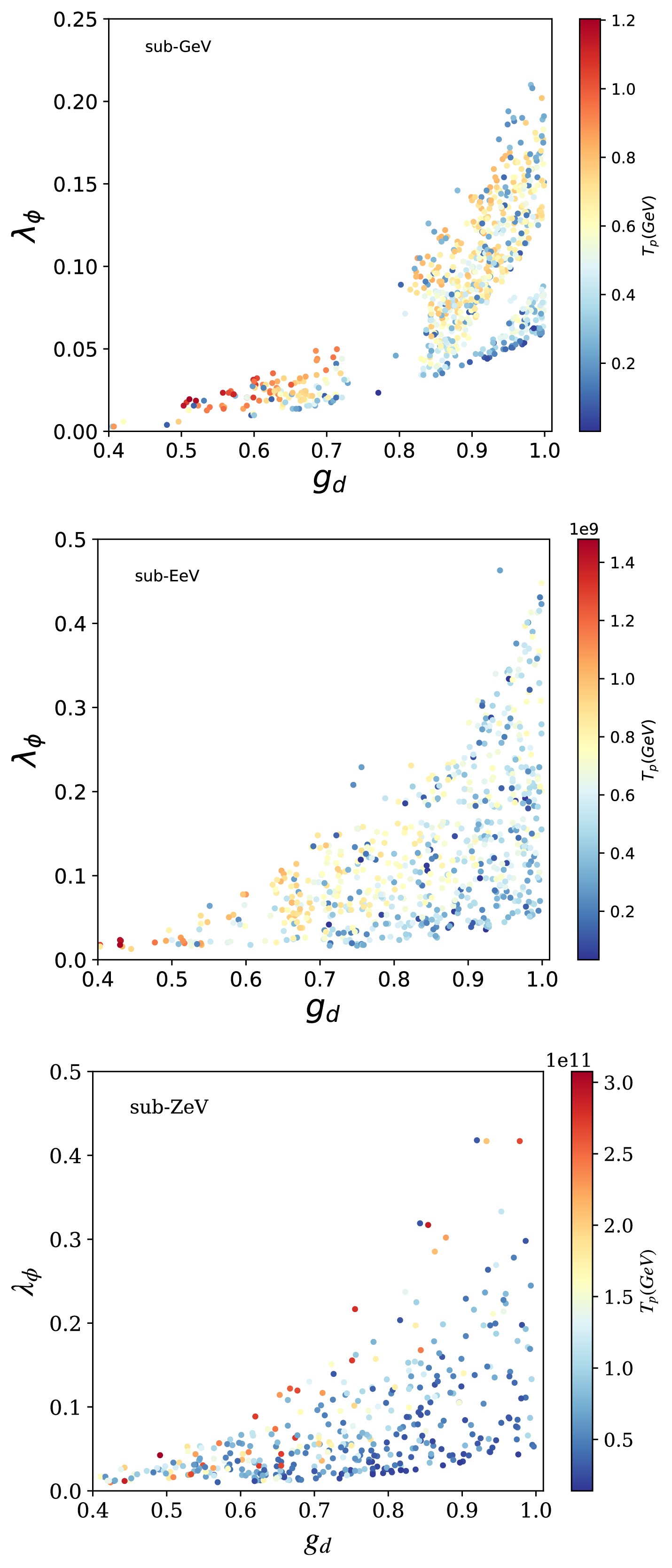

Figure 1.  (color online) Upper, middle, and lower panels show the distribution of viable parameter points in the $ \lambda_\phi - g_d $ plane corresponding to phase transitions occurring at the sub-GeV, sub-EeV, and sub-ZeV energy scales, respectively. The colormap on the right side of the figure represents the percolation temperature $ T_p $ of the phase transition.

During the phase transition, monopoles can form at a rate of approximately $ p \sim \mathcal{O}(10^{-1}) $ as vacuum bubbles collide with each other. Thus, a quantitative relationship can be established to express the number density of monopole $ n_{M} $ in terms of the number density of colliding bubbles $ n_{b} $, which also demonstrates the crucial role of bubble collisions in the monopole production process [83]:

where $ \beta $ represents the duration parameter of the phase transition; for its specific form, see Eq. (19). Hidden monopoles are formed when the $S U(2)_d$ symmetry spontaneously breaks down to $ U(1)_d $. Then, the configurations of the scalar and gauge fields are expressed as follows [47]:

where $ \epsilon^{aij} $ is the totally antisymmetric tensor of rank $ 3 $ with a convention $ \epsilon^{123}=1 $, and $ r=\sqrt{x^2+y^2+z^2} $. In terms of the above configurations and dimensionless variable $ \xi = v_\phi r $, the Lagrangian given in Eq. (1) reduces to

The equations of motion of this system can be written as follows:

where the functions $ H(\xi) $ and $ F(\xi) $ satisfy the following boundary conditions:

Here, $ H(\xi) $ and $ F(\xi) $ are calculated numerically; the monopole mass can be calculated using the following equation:

As discussed above, the mass of the monopole is closely related to the energy scale of the phase transition. In the sub-GeV case, the monopole mass and relic density are minimal, rendering them unobservable. Therefore, in the subsequent discussion, we focus solely on the scenario in which the phase transition occurs at the sub-EeV scale. In the left panel of Fig. 2, we use viable parameters from the sub-GeV and sub-EeV phase transitions to show the profiles of $ H(\xi) $ and $ F(\xi) $ at the percolation temperature $ T_p $. The horizontal axis in this figure is chosen as $ g_d \xi = r m_{w^\prime} $ to represent the core size of a monopole. The right panel of Fig. 2 presents the relation between percolation temperature $ T_p $ and monopole mass $ m_{M} $ calculated using the formulas mentioned above. From this figure, it can be concluded that the monopole mass is approximately proportional to the percolation temperature $ T_p $, following the relation $ m_M \sim 4\pi v_\phi / g_d^2 \sim 4 \pi T_p $ given that most points are concentrated around $ v_\phi(T_p) \sim T_p $ , with $ g_d^2 \sim 1 $.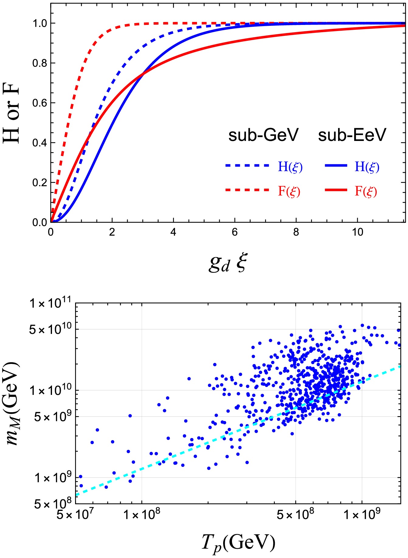

Figure 2.  (color online) Blue and red curves of the upper panel represent the profiles of $ H(\xi) $ and $ F(\xi) $, respectively, where the horizontal axis corresponds to $ g_d \xi = r m_{w^\prime} $. The solid and dashed lines correspond to the feasible phase transition points at different scales. The lower panel shows the relationship between the monopole mass $ m_M $ and percolation temperature $ T_p $. The cyan dashed line represents the value $ 4\pi T_p $, providing a reference scale for comparison.

In our investigation on the influence of the Witten effect on axion mass, we employ a coupling framework consistent with that presented in [31], which describes the interaction between the axion and the dark $ U(1)_d $ gauge field as

where $ e^\prime \equiv 4 \pi / g_d $ is the dark electric gauge coupling. This coupling is inherited following the interaction between the axion and dark $S U(2)_d$ gauge field. Moreover, hidden magnetic monopoles acquire hidden electric charge from this Lagrangian, transforming into particles known as dyons that simultaneously possess both electric and magnetic charges; this is called the Witten effect [84]. Furthermore, considering axions in an electromagnetic field that contains both monopoles and antimonopoles, the axion acquires an effective mass $ m_{a,M} $, which is determined by the number density of monopoles [31, 85]:

where $ n_M(T) $ is the number density of the monopole and $ r_c $ is the core size of the hidden monopole, which can be estimated as the inverse of the mass of the charged gauge bosons generated after the spontaneous symmetry breaking of the $S U(2)_d$ gauge symmetry.

After the formation of monopoles, their number density $ n_M(T) $ is primarily determined by temperature and decreases as the Universe expands. This suggests that the axion mass obtained from the Witten effect correspondingly decreases with the evolution of the universe. Figure 3 shows the dependence of the Witten-effect-induced axion mass $ m_{a,M} $ and monopole mass $ m_M $. As described in Eq. (15), the axion mass $ m_{a,M}[T_p] $ is inversely proportional to the axion decay constant $ f_a $, with most $ m_{a,M}[T_p] $ clustering taking place around $ 10^{-5}\sim 10 $ GeV. At a given $ f_a $, the effective mass $ m_{a,M}[T_p] $ of the axion resulting from monopole coupling grows with the monopole mass $ m_M $ .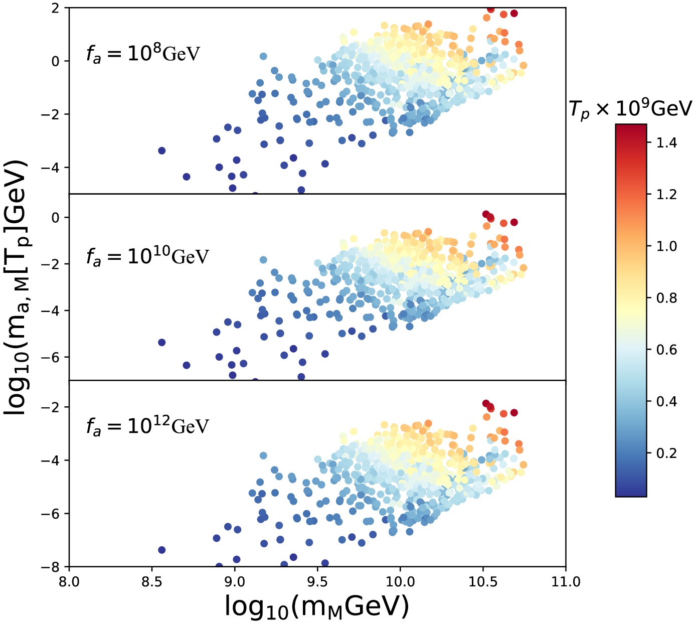

Figure 3.  (color online) Relationship between the monopole mass $ m_M $ and axion mass $ m_{a,M} $ obtained via the Witten effect. From top to bottom, the three figures show the cases in which the axion decay constant $ f_a $ takes the values of $ 10^{8} $ GeV, $ 10^{10} $ GeV, and $ 10^{12} $ GeV, respectively.

Monopoles and antimonopoles experience an attractive interaction that drives their annihilation through a process called ''diffusive capture'' [86−89]. This mechanism can impact the monopole number density $ n_M $. The ''diffusive capture'' process occurs primarily when the mean free path of the monopole, $ \bar\lambda_{\rm mfp} \sim \sqrt{m_M/T}/(BT) $, is smaller than its capture radius, $ r_{\rm cap} \sim h^2/T $ [56, 57]. Here, $ B $ characterizes the drag force induced by the thermal plasma on the monopole [86−89], while $ h=1/g_d $ denotes the hidden magnetic charge of the monopole. The situation we study is the same as that in [34], where $ \bar\lambda_{\rm mfp}>r_{\rm cap} $, meaning that the annihilation of monopoles with anti-monopoles does not affect their number density $ n_M $ generated during the phase transition. Once the monopole number density $ n_M $ and mass $ m_M $ are determined, its relic density can be calculated using the definition of the density parameter as follows:

where $ g_s(T_*)(g_s(T_0)) $ is the effective number of degrees of freedom in entropy at the end of phase transition (today) and $ H_0 $ denotes the present-day Hubble constant.

In the post-inflation scenario, the breaking of global PQ symmetry may lead to the formation of topological defects, such as cosmic strings, which release energy by radiating free axions [90, 91]. After acquiring mass through the Witten effect, the axion can be considered as cold DM. Furthermore, we refer to Ref. [92] to explore the contribution of the KSVZ axion [93, 94] (for $ N_{\rm DW} =1 $) produced by cosmic string radiation to the axion relic density, which can be expressed as

where $ \xi $ and $ \epsilon $ are dimensionless parameters determined by simulation. In the KSVZ model, each domain wall is attached to one string. Such DWs are short-lived and rapidly decay after formation. Consequently, in the subsequent analysis, only the axion radiation from cosmic string is considered. The calculation of axion relic density requires the Witten effect to dominate the axion mass. Based on [92], their values are approximately $ \xi \sim 0.37 $ and $ \epsilon \sim 0.85 $.

In addition, analogous to the effects of the QCD phase transition, the Witten effect contributes to the axion mass and induces the formation of axionic domain walls [46]. Axion strings, arising from the breaking of the $U(1)_{\rm PQ}$ symmetry, are attached to axionic domain walls. This configuration is known as string-wall system, and its decay also contributes to the axion number density [95, 96]. The contribution to the DM relic abundance from the DFSZ axion [94, 97] emitted by domain walls, when the domain wall number $ N_\text{DW} > 1 $, can be described as [98]

where $ \Xi $ denotes coefficient of the bias term $ \Delta V = 2 \Xi v_{\varphi}^4(1-\cos(2\pi/N_{\rm DW})) $. In the DFSZ model, given that the domain walls formed via the Witten effect would immediately dominate the energy density over that of cosmic strings, we only consider the contribution from domain walls when analyzing the axion relic density radiated by this model. To calculate the axion relic density, we adopted a method similar to that reported in Ref. [98], with $ C_d \sim 100 $, $ p \sim 5/4 $, and $ N_{\text{DW}} = 3 $. It is worth noting that the validity of this calculation requires the axion mass to be dominated by the Witten effect rather than the QCD instanton effect prior to domain wall decay. The bias term $ \Delta V $ is determined by the domain wall annihilation time $ t_{\rm dec} $ and domain wall tension $ \sigma_{\rm wall} $, with the specific relation given in Eq. (33).

Figure 4 shows the dependence of the relic density $ \Omega_{a}h^2 $ of KSVZ-like and DFSZ-like axions on monopole abundance $ \Omega_M h^2 $ and decay constant $ f_a $. To estimate the number density of KSVZ-like axions, we adopted the method reported in Ref. [92] until the axion mass approaches the Hubble constant $ m_{a,M}[T_w]\sim3H[T_w] $, at which the axion field begins to behave as DM should. At this epoch prior to the QCD phase transition, the axion mass originates solely from the Witten effect. The black dashed line in Fig. 4 indicates the experimentally observed relic density of DM $ \Omega_{\rm DM}h^2\sim0.12 $ [99]. As previously discussed, both monopoles and axions radiated from topological defects (particularly cosmic strings and domain walls) can serve as viable DM candidates that contribute to the DM relic density. Notably, while cosmic strings generate a substantially larger axion population compared to domain walls, both contributions remain subdominant relative to that from dark monopoles. Current observational constraints on the DM relic density exclude parameter regions with larger axion decay constants $ f_a $in the KSVZ-like model, given that these values would lead to overproduction of axion DM beyond the observed limit of DM. The right panel of Fig. 4 includes triangles and circles to denote the axion radiation contributions from domain walls at different energy scales. When considering only the Witten effect contribution to the axion mass, the results show that domain wall annihilation at the electroweak scale yields axion relic densities that substantially exceed those from the QCD scale. Similar to the cosmic string scenario, domain walls exhibit a positive correlation between axion production and the decay constant $ f_a $. While the axion relic density remains negligible relative to that of dark monopoles at smaller decay constant (e.g.,$ f_a=10^8 $ GeV), it becomes comparable in magnitude at $ f_a=10^{10} $ GeV.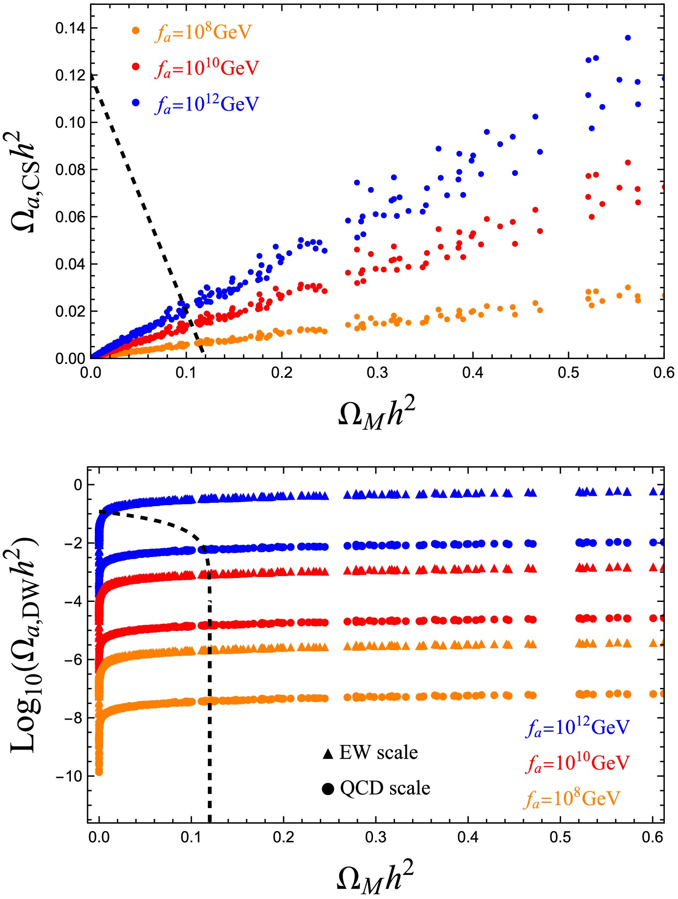

Figure 4.  (color online) Upper (lower) panel shows the relationship between the abundances of KSVZ-like axions (DFSZ-like axions) and monopoles. The orange, red, and blue points represent cases in which the axion decay constant takes values of$ f_a=10^{8} $ GeV, $ f_a=10^{10} $GeV, and $ f_a=10^{12} $ GeV, respectively. The dashed black line corresponds to the experimentally measured DM density.

The existence of dark phase transitions and domain wall collapse processes suggests that GWs emitted by these events could provide valuable insights into probing new physics models. Our primary focus is on the stochastic GW background, particularly when its peak frequency lies within the nanohertz range detectable by PTA experiments. Accordingly, we investigated domain wall GWs in the sub-EeV scenario and phase transition GWs in the sub-GeV scenario. Additionally, we examined the constraints imposed by CMB observations on relativistic particles in the dark sector, commonly referred to as dark radiation.

Evaluating the GW spectrum produced during a first-order phase transition requires determining the phase transition strength parameter $ \alpha $and duration parameter $ \beta $, defined as follows:

where $ \rho_{\text{DR}}=\pi^2 g_{\rm DR} T^4/30 $ is the plasma energy density, and the vacuum energy released during the phase transition is defined as [100]

Moreover, in subsequent discussions, we consider the calculations at $ T_*=T_p $ while adopting the notation $ T_* $ for consistency in description.

In this study, we followed the method outlined in [23] to estimate the GWs generated during the dark first-order phase transition, taking into account contributions from bubble collisions [101], sound waves [102, 103], and turbulence [104, 105]:

where

Here, $ \Omega_{\rm rad,0} h^2= 4.16 \times 10^{-5} $ [106] , where $ h $ is the reduced Hubble parameter and $ \alpha^\prime $ can be defined as

where $ \rho_{\rm rad,tot}(T_*) $ is the total radiation energy density just before the phase transition.

where $ f $ is the frequency today, $ \Upsilon = (1-1/{\sqrt{1+2 t_{\rm sw} H_*}}) $ represents the suppression factor, $ \tau_{sw} $ represents the sound wave duration during the phase transition, as discussed in Ref. [107], $ \tau_{sw}= {\min}\left[{1}/{H_*}, R_*/{\bar{U}_f}\right] $, $ H_*R_*= v_w(8\pi)^{1/3}/(\beta/H_*) $, the root-mean-square fluid velocity $ \bar{U}_f $ can be approximated as [108−110] $ \bar{U}_f^2\approx3\kappa_\nu\alpha^\prime/ {4(1+\alpha^\prime)}\; $, and $ h_* $ is the Hubble parameter at $ T_* $ expressed as

The peak frequencies of three sources, namely $ f_{\rm bubble} $, $ f_{\rm sw} $, and $ f_{\rm turb} $ , can be expressed as

To prevent the universe from "over-closing," a biased potential $ \Delta V $ can be introduced to ensure that domain walls collapse after their formation. Furthermore, the GW signals generated during the collapse of these domain walls offer a novel avenue to test this process experimentally. This mechanism provides a new theoretical framework and experimental direction for investigating the properties of cosmological defects and their potential observational signatures. The energy released during this process is radiated as GWs, and the peak frequency and peak amplitude of these waves at the present time $ t_0 $ can be estimated as follows [111, 112]:

where $ \sigma_{\rm wall}\sim c_a m_{a,M}(T) f^2_a $ and $ c_a = \mathcal{O}(1) $ is a numerical constant [45]. The bias term $ \Delta V $ introduced in Eqs. (31) and (32) explicitly breaks the discrete symmetry, which determines the decay time of the domain wall:

Furthermore, the constraints are such that the domain wall decay must occur before they "overclose" the Universe and Big Bang Nucleosynthesis [113, 114]. These conditions can be expressed as follows:

Naturally, the bias term exhibits both lower and upper bounds. Specifically, the magnitude of the bias term must be much smaller than the potential around the core of the domain walls, ensuring that the discrete symmetry is approximately preserved. In this study, based on the case of $ N_{\text{dw}} = 3 $, we selected the area parameter $ \mathcal{A} = 1.2 $ [111] and efficiency parameter $ \tilde{\epsilon}_{\mathrm{gw}} = 0.7 $ [112], which are consistent with the discrete symmetry. According to the literature [112], after calculating the peak frequency and peak amplitude of the GWs, the domain wall GW power spectrum can be approximated as a piecewise function as follows: for$ f < f^{\rm dw}_{\text{peak}} $, $ \Omega_{\rm GW}^{\text{dw}} h^2 \propto f^3 $, and for $ f \geq f^{\rm dw}_{\text{peak}} $, $ \Omega_{\rm GW}^{\text{dw}} h^2 \propto f^{-1} $.

As shown in Fig. 5, the peak frequency of axionic domain walls, $ f_{\text{peak}} $, rises with a decreasing mass $ m_{a,M} $ and falls with an increasing decay constant $ f_a $. Moreover, the peak frequency is positively correlated with $ \Delta V $. In contrast, the peak amplitude $ \Omega_{{\rm GW}{\rm peak}} $ varies inversely with the peak frequency. It increases with the axion mass $ m_{a,M} $ and decay constant $ f_a $ and is negatively correlated with the bias term $ \Delta V $. The mass of axions has a decisive impact on the peak amplitude and peak frequency of domain wall GWs. The axion mass $ m_{a,M} $, contributed by the Witten effect, decreases significantly with the temperature. The decay time of axionic domain walls determines the peak frequency of the generated GWs.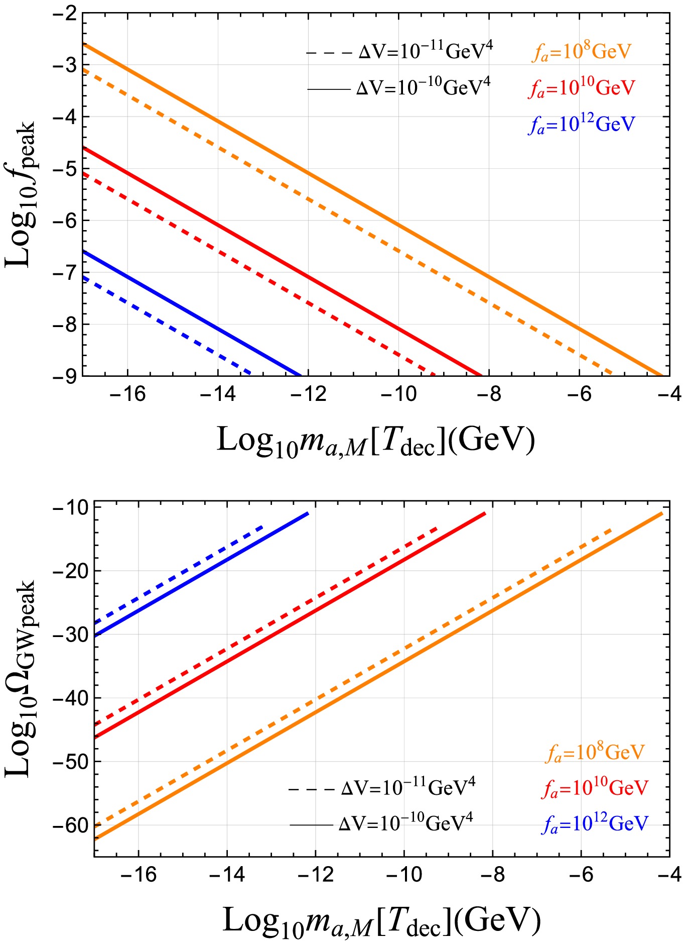

Figure 5.  (color online) Upper (lower) panel shows the relationship between axion mass and peak frequency (peak amplitude). As in Fig. 3, the orange, red, and blue lines correspond to scenarios with different axion decay constants. In addition, the solid and dashed lines represent the results for different values of $ \Delta V $.

We present the predictions for phase-transition GWs and domain wall collapse GWs at several benchmark points from Table 1 in Fig. 6. As shown in this figure, both types of GWs have peak frequencies in the nano-hertz range. However, the peak amplitude of GWs from phase transition in the sub-GeV scenario is significantly higher than that of the GWs from domain walls in the sub-ZeV scenario. Both the phase transition GWs and domain wall GWs could be detectable by current PTA experiments as well as future space-based GW detectors. However, in the sub-EeV scenario, the axion mass $ m_{a,M} $ determined by the Witten effect becomes extremely small during domain wall decay. Consequently, the peak amplitude of the resulting axionic domain wall GWs lies well below the sensitivity range of current GW experiments. Note also that, according to Ref. [92], the GW power spectra of the axion string that can be detected by recent PTA experiments has been excluded as a result of setting the DM constraint.

	$ g_{d} $	$ \lambda_{\phi} $	$ \lambda_{\varphi \phi} $	$ T_p $ (GeV)	$ \beta/H_p $	$ \alpha[T_p] $
$\rm BM_1 $	0.771	0.023	$ 3.91\times10^{-26} $	0.001	76.47	35.57
$\rm BM_2 $	0.972	0.054	$ 1.05\times10^{-22} $	0.038	23.36	114.67
$\rm BM_3 $	0.927	0.046	$ 4.49\times10^{-23} $	0.038	41.24	25.84
$\rm BM_4 $	0.648	0.015	$ 2.31\times 10^{-3} $	$ 1.422\times10^{11} $	43306.7	0.119
$\rm BM_5 $	0.387	0.017	$ 3.34\times10^{-3} $	$ 3.057\times10^{11} $	35918.4	$ 2.83\times 10^{-3} $
$\rm BM_6 $	0.631	0.0013	$ 3.12\times10^{-3} $	$ 6.428\times10^{11} $	80826.9	0.012

Table 1.  Benchmarks in Fig. 6.

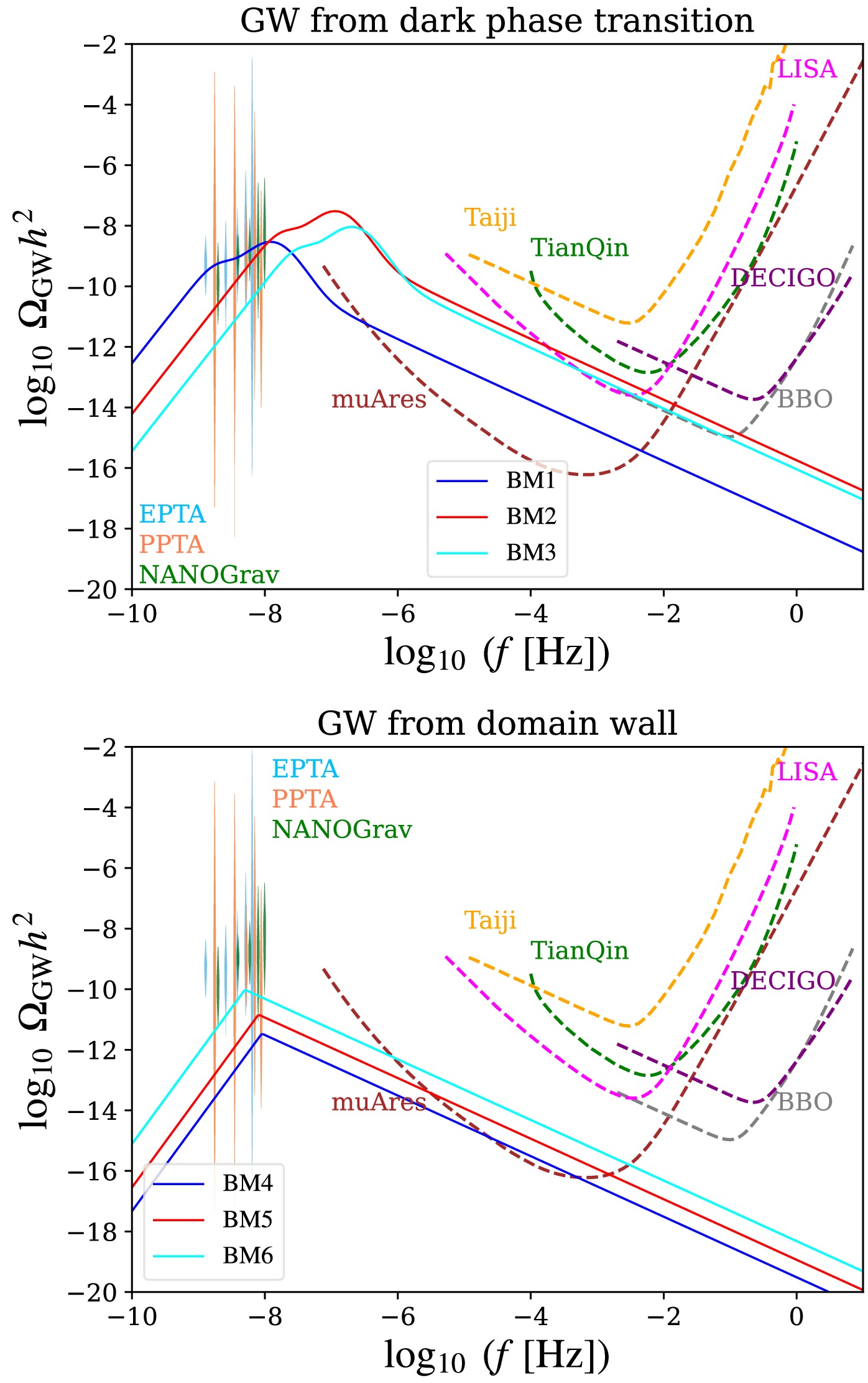
Figure 6.  (color online) Upper panel shows the GW energy spectra generated by dark phase transitions for the first three benchmark points listed in Table 1. Meanwhile, the lower panel depicts the GW energy spectra resulting from axion domain wall decay for the last three benchmark points in Table 1. The violin plots represent data from three experiments: EPTA [115], PPTA [116], and NANOGrav [117]. Moreover the brown, gray, orange, green, purple, and gray dashed lines show the projected sensitivity of the muAres [118], LISA [119, 120], Taiji [121, 122], TianQin [123], DECIGO [124−126], and BBO [127] collaboration, respectively.

Table 1 presents six viable parameter points for the first-order phase transition. The first three correspond to phase transitions at the sub-GeV scale, while the last three are associated with sub-ZeV scale phase transitions.

In this study, we assumed that the dark sector does not directly couple to the visible sector but is connected through the axion as a mediator particle. In the sub-GeV scenario, the coupling between the dark sector and the axion is extremely weak, implying that the interactions between the dark and visible sectors are negligible. In the sub-EeV and sub-ZeV scenarios, the dark and visible sectors decouple from thermal equilibrium after the axion decouples from the SM. Given that the coupling strength between the axion and the SM is significantly suppressed by $ f_a $, it can be inferred that the decoupling between the dark and visible sectors occurs before the EW phase transition. Furthermore, after the first-order phase transition, it is reasonable to assume that the entropy of the dark and visible sectors are separately conserved, which allows us to write the following relation:

where $ g^{sm}(T)(g^{sm}_{s}(T)) $ and $ g^d(T)(g^d_{s}(T)) $ are the relativistic degrees of freedom for the energy (entropy) densities in the visible and dark sectors. When we assume that the first-order phase transition does not occur under supercooling conditions, the extra effective number of relativistic particles can be reasonably expressed as follows [15]:

where $ R=s_d(T)/s_{sm}(T)|_{T>T_{pt}} $ and the subscript 0 represents the value at the recombination epoch. After the breaking of dark $ S U(2)_d $ symmetry, the dark photon remains massless. Following the QCD phase transition, the axion mass originates from two sources: the misalignment mechanism and the Witten effect, with the misalignment contribution being dominant at this stage. Consequently, in this model, only the dark photon should be considered as a component of dark radiation, yielding $ \Delta N_{\text{eff}}=0.40 $. Current observations from Planck and BBO establish the constraint [99, 128] $ N_{\text{eff}} = 3.27\pm0.15 $. In the SM, $ N_{\rm eff}=3.046 $. Moreover, Refs. [99, 129, 130] suggest that $ \Delta N_{\text{eff}} \sim 0.4-0.5 $ could effectively alleviate tension in the Hubble constant.

In this study, we investigated the generation of hidden monopoles through spontaneous breaking of dark $ SU(2)_d $ symmetry, focusing on their impact on axion mass and the feasibility of monopoles and axions as DM candidates. Furthermore, we assess the potential of current GW experiments to detect stochastic GW backgrounds originating from dark $S U(2)_d$ phase transitions and axionic domain wall collapse. Our study indicates that in the sub-EeV scenario, the mass of hidden monopoles is approximately $ 10^{10} $ GeV, rendering them viable DM candidates. Furthermore, within the percolation temperature, the axion mass generated exclusively through the Witten effect spans from $ \mathcal{O}(10^{-5}) $ GeV to $ \mathcal{O}(10) $ GeV, with its precise value being determined by the axion decay constant $ f_a $. However, the axion mass contributed by monopoles diminishes gradually as the universe expands. In most regions of the parameter space, axions can serve as part of DM. In this study, we investigated scenarios where domain wall annihilation occurs at either EW or QCD scales. Domain wall annihilation at the electroweak scale, when considering only Witten-effect-derived axion masses, generates axion relic densities that significantly surpass those resulting from annihilation at the QCD scale. Furthermore, the relic density of DFSZ-like axions exhibits a distinct positive correlation with the decay constant $ f_a $. Meanwhile, concerning axions radiated by cosmic strings, their relic density in most of the viable phase-transition parameter space is below the current observational limits on the DM relic density. In addition to axions generated via cosmic string or domain wall emission, hidden monopoles formed during the phase transition can jointly explain the observed DM relic abundance, with the monopole number density surpassing that of axions from either production progress. In the sub-GeV scenario, the monopole-induced contribution to the axion mass becomes negligible compared to the contribution from non-perturbative QCD effects. However, in the sub-ZeV scenario, the mass of the monopole and the axion mass contributed by the Witten effect are significantly larger than those in the sub-EeV scenario.

Additionally, it is worth noting that in this study we primarily examined stochastic GW backgrounds originating from the early universe, with peak frequencies in the nano-hertz range. If the $ S U(2)_d $ symmetry breaking occurs near an energy scale of $ \sim \mathcal{O}(100) $ MeV, immediately following the QCD phase transition, the resulting phase transition GWs would fall within the nanohertz frequency band. Within this framework, the coupling between the axion and scalar $ \phi $ is exceedingly small. This finding potentially explains the low-frequency GW signals observed by the EPTA, PPTA, and NANOGrav collaborations and paves the way for exploring new physics models that incorporate the dark sector. Furthermore, although the collapse of axionic domain walls can produce a stochastic GW background in the nanohertz frequency range, the peak amplitude of these GWs is determined by the axion mass. The peak amplitude of nanohertz GWs from domain walls in the sub-ZeV case is substantially higher than in the sub-GeV case, making them potentially detectable by current PTA experiments as well as future space-based GW detectors.

Moreover, if the axionic domain wall interacts with lepton or baryon currents, their formation and collapse could generate lepton or baryon number asymmetry, offering a potential explanation for the observed baryon asymmetry in the universe. This mechanism, referred to as ''DW-genesis'' [131, 132], represents a novel production mechanism. Meanwhile, the contribution of the Witten effect to the axion mass could influence the axiogenesis process [133, 134], where the cosmological net baryon number is generated through the rotation of the QCD axion. This topic will be addressed in future studies.

The Coleman-Weinberg contribution can be expressed as [135]

where $ b=0(1) $ for bosons (fermions), $ \Lambda_{UV} $ is the $ \rm\overline{MS} $ renormalization scale, $ g_i = \{ 1,1,6 \} $ for $ \{ \phi, G_{W^\prime}, W^\prime \} $ in this model, $ C_i = 5/6 $ for the gauge boson, and $ C_i = 3/2 $ for others.

where the corresponding coefficients are calculated from

The one-loop finite temperature corrections can be written as [136]

where the functions $ J_{B} $ are

with $ y\equiv m_{i}^2(\phi)/T^2 $.

The thermal integrals $ J_{B} $ defined in Eq. (41) can be expressed as an infinite series involving modified Bessel functions of the second kind, $ K_{n} (x) $ , with $ n=2 $ [137]:

The daisy term $ V_{1}^{\rm daisy}(\phi,T) $ is given by [138, 139]

where the finite temperature corrections are expressed as