Revisiting axion-like particle couplings to electroweak gauge bosons

Probing new pseudoscalar particles with masses below the electroweak scale predicted in some well-motivated extensions of the standard model (SM) plays an important role in particle physics. A notable example is axion-like particles (ALP), which are an extension of original quantum chromodynamics (QCD) axions from the spontaneous breaking of Peccei-Quinn symmetry [1−6]. As a generalization, ALP can be realized in a variety of new physics scenarios with a significantly larger parameter space, see [7−10] for a review. This enables a rich phenomenology, investigated in both low-energy [11−14] and high-energy experiments [15−17]. In addition, many new experiments are conducted, including IBS-CAPP MAX [18], oscillating resonant group axion (ORGAN) [19], any light particle search II (ALPS II) [20], CERN axion solar telescope (CAST) [21], and NEON [22].

In recent years, increasingly precise predictions [23−36] and experimental observations [37] for meson flavor-changing neutral current (FCNC) decays have revealed several notable discrepancies. For example, Belle-II uses an integrated luminosity 362 fb^–1 to measure $ {\rm{Br}}(B^+ \to K^+ \nu \bar{\nu})=23\pm 5^{+5}_{-4} $, which exceeds the SM prediction by $ 2.7\sigma $ significance [38]. Similarly, the NA62 collaboration [39, 40] reported precise measurements of the branching ratio $ {\rm{Br}}(K^+\to \pi^+ \nu\bar{\nu}) $, significantly improving on the previous results from the E949 experiment [41]. Owing to the presence of invisible final-state neutrinos, these decay signals can be mimicked by ALP, which would appear as missing-energy events. Table 2 summarizes recent results and refined experimental upper limits for meson decays from various experiments, which motivate us to update and extend previous analyses on meson FCNC processes involving an ALP. Several mechanisms have been proposed to construct flavor-changing ALP interactions [42−50]. ALP interactions with $ W^\pm $ bosons can induce FCNC processes at one loop level [44], which constitutes the primary focus of this work.

quark transition	Observable	SM prediction ($ \times 10^{-6} $)	Experimental data ($ \times 10^{-6} $)
$ s\to d $	$ {\rm Br}(K^+ \to \pi^+ \nu \bar{\nu}) $	$ (8.42\pm 0.61)\times 10^{-5} $ [53]	$ (13.0^{+3.3}_{-3.0})\times 10^{-5} $(NA62 [39, 40])
	$ {\rm Br}(K_L \to \pi^0 \nu \bar{\nu}) $	$ (3.41\pm 0.45)\times 10^{-5} $ [53]	$<3\times 10^{-3} $(KOTO [54])
	$ {\rm Br}(K^+ \to \pi^+ ee) $	$ 0.3\pm0.03 $ [55]	$ 0.3\pm0.009 $(NA48 [37])
	$ {\rm Br}(K^+ \to \pi^+ \mu\mu) $	$ (9.4\pm0.6)\times 10^{-2} $ [55]	$ (9.17\pm0.14)\times 10^{-2} $(NA62 [37])
	$ {\rm Br}(K_L \to \pi^0 ee) $	$ (3.38\pm0.92)\times 10^{-5} $ [56]	$<2.8\times 10^{-4} $(KTEV [57])
	$ {\rm Br}(K_L \to \pi^0 \mu\mu) $	$ (1.39\pm 0.27)\times 10^{-5} $ [56]	$<3.8\times 10^{-4} $(KTEV [58])
$ b\to d $	$ {\rm Br}(B^+ \to \pi^+ \nu \bar{\nu}) $	$ 0.140\pm0.018 $ [53]	$<14 $(Belle II [59])
	$ {\rm Br}(B^0 \to \pi^0 \nu \bar{\nu}) $	$ 0.0652\pm 0.0085 $ [53]	$<9 $(Belle II [59])
	$ {\rm Br}(B^+ \to \rho^+ \nu \bar{\nu}) $	$ 0.406\pm 0.079 $ [53]	$<30 $(Belle II [59])
	$ {\rm Br}(B^0 \to \rho^0 \nu \bar{\nu}) $	$ 0.189\pm 0.036 $ [53]	$<40 $(Belle II [59])
	$ {\rm Br}(B^+ \to \pi^+ ee) $	$ (1.95\pm0.61)\times 10^{-2} $ [60]	$<5.4\times 10^{-2} $(Belle-II [61])
	$ {\rm Br}(B^0 \to \pi^0 ee) $	$ (0.91\pm0.34)\times 10^{-2} $ [60]	$<7.9\times 10^{-2} $(Belle-II [61])
	$ {\rm Br}(B^+ \to \rho^+ ee) $	O(0.02) [37]	$<0.467 $(Belle-II [61])
	$ {\rm Br}(B^+ \to \pi^+ \mu\mu) $	$ (1.95\pm0.61)\times 10^{-2} $ [60]	$ (1.78\pm0.23)\times 10^{-2} $(LHCb [37])
	$ {\rm Br}(B^0 \to \pi^0 \mu\mu) $	$ (0.91\pm0.34)\times 10^{-2} $ [60]	$<5.9\times 10^{-2} $(Belle-II [61])
	$ {\rm Br}(B^+ \to \rho^+ \mu\mu) $	O(0.02) [37]	$<0.381 $(Belle II [61])
	$ {\rm Br}(B \to \mu \mu) $	$ (1.03\pm0.05)\times 10^{-4} $ [62]	$<1.5\times 10^{-4} $(CMS [63])
	$ {\rm Br}(B \to \tau \tau) $	0.03 [64]	$<2100 $(CMS [63])
$ b\to s $	$ {\rm Br}(B^+ \to K^+ \nu \bar{\nu}) $	$ (4.97\pm0.37) $ (HPQCD[65])	$ 23\pm 5^{+5}_{-4} $(Belle II [38])
	$ {\rm Br}(B^0 \to K^0 \nu \bar{\nu}) $	$ 3.85\pm0.52 $ [53]	$<26 $(Belle [66])
	$ {\rm Br}(B^+ \to K^{*+} \nu \bar{\nu}) $	$ 9.79\pm 1.43^* $ [67]	$<61 $(Belle [66])
	$ {\rm Br}(B^0 \to K^{*0} \nu \bar{\nu}) $	$ 9.05\pm 1.37 $ [67]	$<18 $(Belle [66])
	$ {\rm Br}(B_s \to \phi \nu \bar{\nu}) $	$ 9.93\pm 0.72 $ [53]	$<5400 $(LEP DELPHI [68])
	$ {\rm Br}(B^+ \to K^+ ee) $	$ 0.191\pm0.015 $ [56]	$ 0.56\pm 0.06 $(Belle [37])
	$ {\rm Br}(B^0 \to K^0 ee) $	$ 0.51\pm0.16 $ [60]	$ 0.25\pm 0.11 $(Belle [37])
	$ {\rm Br}(B \to K^* ee) $	$ 0.239\pm0.028 $ [56]	$ 1.42\pm 0.49 $(Belle-II [69])
	$ {\rm Br}(B^+ \to K^+ \mu\mu) $	$ 0.191\pm0.015 $ [56]	$ 0.1242\pm0.0068 $(CMS [70])
	$ {\rm Br}(B^0 \to K^0 \mu\mu) $	$ 0.51\pm0.16 $ [60]	$ 0.339\pm0.035 $(Belle [37])
	$ {\rm Br}(B \to K^* \mu\mu) $	$ 0.239\pm0.028 $ [56]	$ 1.19\pm0.32 $(Belle-II [69])
	$ {\rm Br}(B_s \to \phi \mu\mu) $	$ (0.27\pm0.025) $ [56]	$ 0.814\pm0.047 $(LHCb [71])
	$ {\rm Br}(B^+ \to K^+ \tau\tau) $	$ 0.12\pm0.032 $ [60]	$<2250 $(BaBar [72])
	$ {\rm Br}(B_s \to \mu\mu) $	$ (3.78\pm 0.15)\times 10^{-3} $ [56]	$ (3.34\pm0.27)\times 10^{-3} $(CMS [63])
	$ {\rm Br}(B_s \to \tau\tau) $	0.8 [64]	$<6800 $(LHCb [73])

Table 2.  SM predictions and experimental measurements of meson decays. Upper limits are all given at 90% confidence level (CL). $ * $ denotes the contribution is obtained by subtracting the tree-level effect from $ B^+ \to \tau^+(\to K^{*+} \bar{\nu}) \nu $, $ [(10.86\pm 1.43)-(1.07\pm 0.10)]\times 10^{-6} $.

In this paper, we provide an updated and extended analysis on the experimental limits of ALP couplings to electroweak gauge bosons across the ALP mass range from MeV to 100 GeV. As mentioned, the ALP-$ W^\pm $ couplings can induce flavor-changing ALP-quark interactions $ q_i-q_j-a $ at the one-loop level. Associated physical processes such as rare meson decays and neutral meson mixing are analyzed to determine excluded regions in the ALP parameter space with state-of-the-art SM predictions and new experimental data. Pb-Pb collisions also provide constraints in the ALP mass range $ m_a\in [5,100] $ GeV. In addition, these couplings affect Z-boson precision measurements, including $ \Gamma_Z $, $ Z\to \gamma a $ with subsequent decays, and the oblique parameters (S, T, U). Moreover, we analyze future experimental sensitivities from lepton colliders (e.g., CEPC and FCC-ee) operating at the Z-pole and the proposed search for hidden particles (SHiP) experiment. To provide a comprehensive basis for comparison, we consider four distinctive scenarios from two independent ALP couplings, namely the ALP-$ S U(2)_L $ gauge boson coupling $ g_{aW} $ and the ALP-hypercharge gauge boson coupling $ g_{aB} $.

● $ g_{a\gamma\gamma}=0 $: suppress ALP-photon interaction by cancellation between $ g_{aW} $ and $ g_{aB} $, called photophobic ALP [51];

● $ g_{aB}=0 $: turn off the coupling with $ U(1)_Y $ field;

● $ g_{aB}*g_{aW}>0 $: the same sign to enhance the ALP-photon coupling;

● $ g_{aW}=0 $: turn off the coupling with $ S U(2)_L $ field.

The rest of this paper is organized as follows. In Section II, we discuss low energy effective couplings of an ALP induced from the ALP couplings to electroweak gauge bosons at an ultraviolet (UV) scale. Section III presents a comprehensive list of phenomenological observables relevant for probing the ALP couplings to electroweak gauge bosons. In Section IV, we discuss our results on current and future experimental limits on the ALP-electroweak gauge boson couplings. Finally, in Section V, we present our conclusions.

The general ALP couplings with gauge bosons are written as

where a=1,2,3 represents the SU(2) index, and $ W^{\mu\nu} $ ($ B^{\mu\nu} $) represents $ S U(2)_L $ ($ U(1)_Y $) gauge bosons. $ \tilde{W}^{\mu\nu}(\tilde{B}^{\mu\nu}) $ are the dual field strength tensors. After symmetry breaking, the fields W and B are transformed into the physical fields $ \gamma $ and Z,

where $ c_W \equiv \cos \theta_W $ and $ s_W \equiv \sin \theta_W $ with $ \theta_W $ are the weak Weinberg mixing angle. By adopting the above transformation in Eq. (1), the ALP-gauge boson interactions can be written as

where $ F_{\mu\nu} $, $ W_{\mu\nu} $, and $ Z_{\mu\nu} $ represent the field strength tensors of the photon, $ W^\pm $, and Z bosons, respectively. Furthermore, the coupling coefficients can be expressed in terms of $ g_{aW} $ and $ g_{aB} $

In addition, the ALP-$ W^\pm $ couplings induce the following interaction vertex

where $ p_{W\alpha} $ and $ p_{W\beta} $ represent the four momentum of the W bosons. The a-W-W interaction can contribute to the flavor-changing down-quark interaction as shown in Fig. 1.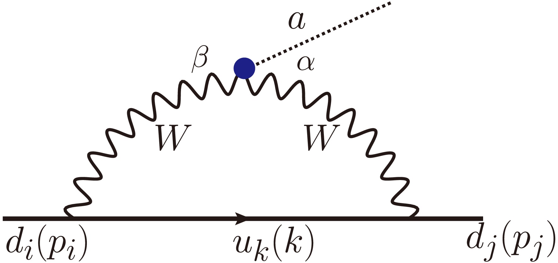

Figure 1.  (color online) Flavor-changing $ a-d_i-d_j $ interaction ($ i\neq j $). The symbols in brackets represent the corresponding momentum.

Additionally, the SM charged vector-current interaction mediated by $ W^\pm $ bosons are expressed by

where $ g $ represents the gauge coupling constant of the $ S U(2)_L $ gauge group. In addition, the subscript $ L $ represents the projection on the left. Furthermore, the Cabibbo-Kobayashi-Maskawa (CKM) mixing matrix $ V_{\rm CKM} $ is parameterized by three rotation angles and one phase

where the corresponding values are shown in Table 1.

parameters	input/GeV	parameters	input numbers
$ m_Z $	91	$ G_{\rm F} $	$ 1.1664\times 10^{-5} $GeV-2
$ m_W $	80	$ s_W^2 $	0.23129
$ m_t $	173	$ \Gamma_{B_s} $	$ 65.81\times 10^{10}s^{-1} $
$ m_b $	4.183	$ \Gamma_{B^+} $	$ 1/1638\times 10^{15}s^{-1} $
$ m_c $	1.2730	$ \Gamma_{B^0} $	$ 1/1517\times 10^{15}s^{-1} $
$ m_{e} $	$ 0.511\times 10^{-3} $	$ \Gamma_{K^+} $	$ 1/1.2380\times 10^{8}s^{-1} $
$ m_\mu $	$ 0.10566 $	$ \Gamma_{K} $	$ 1/5.116\times 10^{8}s^{-1} $
$ m_{\tau} $	1.777
$ m_{B_s} $	5.36693	$ \sin\theta_{12} $	0.22501
$ m_{B^+} $	5.27941	$ \sin\theta_{13} $	0.003732
$ m_{B^0} $	5.27972	$ \sin\theta_{23} $	0.04183
$ m_{K^+} $	$ 0.493677 $	$ \delta $	1.147
$ m_{K_L} $	$ 0.497611 $
$ m_{\pi^+} $	$ 0.13957 $	$ f_K\sqrt{B_K} $	0.132GeV
$ m_{\pi^0} $	$ 0.1349768 $	$ f_{B_d}\sqrt{B_d} $	225MeV
$ m_{\rho^0} $	$ 0.770 $	$ f_{B_s}\sqrt{B_s} $	274 MeV
$ m_{\phi} $	$ 1.020 $

Table 1.  Relevant parameters and input numbers.

By combing the interactions in Eqs. (5) and (6), we can write down the amplitude in Fig. 1 as

where $ i\neq j $ implies flavor-changing interactions. At first glance, the amplitude should be UV divergent when analyzing the loop integral. After dimensional regularization, the divergent term should be proportional to

where $ d=4-\epsilon $. This divergence should be eliminated by the renormalization. Before the renormalization, we analyze the structure of the divergent terms. We find that the divergence term is independent of quark mass. When summing over up-type quarks (u, c, t), we naturally obtain the CKM matrix as

This shows that the divergences disappear because of the unitarity of the CKM matrix when we consider all three generation up-type quarks in the propagator.

By ignoring the quark masses of the initial and final states and using $ \epsilon^{\mu\nu\alpha\beta}\gamma_\nu \gamma_\alpha \gamma_\beta=6{\rm i}\gamma^\mu\gamma^5 $, the finite term with $ \bar{u}_j \not {p}_a P_L u_i $ can be obtained approximately as

where $ \lambda=m_k^2/m_W^2 $. Note that the first term (–1) also disappears owing to CKM unitarity. Therefore, by combining the corresponding coefficients, we obtain an effective interaction [42]

where $ G_{\rm F}=1.1664\times 10^{-5} $ GeV^–2 represents the Fermi constant. $ V_{ij} $ represents the relevant CKM matrix. Note that for $ x\ll1 $, we obtain

The interaction is proportional to $ m_\alpha^2/m_W^2 $ for $ m_\alpha<<m_W $.

Therefore, for the above flavor-changing couplings, the result is finite and only depends on the IR value of the effective coupling. Although the individual diagrams in Fig. 1 are UV divergent, the divergences cancel out when intermediate up-type quark flavors $ u_k $are summed up. This interesting feature can be attributed to two points: the unitarity of the CKM matrix and the quark-mass independent divergences. This is in contrast with models possessing a direct ALP-quark coupling, wherein the FCNC rate is sensitive to UV completion [42, 52].

By further using the equation of motion, the above effective interaction for the on-shell fermions can be converted into

This form shows that the main interactions should be RH chiral quark structures because of $ m_{d_i}>>m_{d_j} $.

The above flavor-changing quark interaction induced by a-W-W coupling contributes to different observables. In this part, we drive the experimental constraints on the coupling $ g_{aW} $ and ALP mass $ m_a $, and we discuss possible ALP explanations for the experimental anomalies.

The above quark couplings $ a-d_i-d_j $ will mediate FCNC rare decays of heavy-flavor mesons at the tree level. The rare mesons that decay into mono-energetic final state mesons and on-shell ALPs, $ M_1\to M_2 a $, are the most sensitive probes of flavor-violating ALP couplings. This indicates that relevant interactions are constrained by the corresponding physical processes as shown in Table 2.

We exclusively focus on the bounds derived on the flavor-changing ALP couplings. For estimating the transition matrix element of meson rare decays, we take the B meson as an example with the form factors as [74, 75]

where $ P $ and $ V $ correspond to pseudo-scalar and vector state mesons, respectively. For the decay $ B\to K^*a $ , the $ K^* $ meson actually only has longitudinal polarization contribution because the ALP is a pseudoscalar particle. For the kaon rare decays, we can estimate its amplitude under the vertor current conserved assumption [44]. Note that the matrix element for $ K^0\to \pi^0 a $ is related to $ K^\pm\to \pi^\pm a $ by isospin symmetry. Therefore, the matrix element for the $ K_L(K_S) $ mass eigenstate is obtained by taking the imaginary (real) part of the $ K^\pm\to \pi^\pm a $ matrix element [76]. Therefore, the corresponding decays for B and K mesons are expressed by

where $ \lambda(x,y)=[1-(x+y)^2][1-(x-y)^2] $. Note that the factor $ 1/2 $ in $ \Gamma(\bar{B}^0\to \pi^0 a) $ comes from the quark components $ \pi^0=(\bar{u} u+\bar{d} d)/ \sqrt{2} $. The other decay processes can be obtained by the corresponding transformations on the masses and form factors. Using light-cone sum rules [74, 75], the corresponding expressions are

Note that the above forms fix the axion mass unit with $ m_a/{\rm{GeV}} $. In all cases, these couplings are renormalized at the scale of the measurement; however, the flavor-changing ALP couplings do not run below the weak scale, and therefore it is equivalent to using couplings renormalized at the weak scale. In addition, we expect that the subprocesses of the type $ B^-\to \pi^-a $ via ALP-pion mixing make subdominant contributions to the $ B^-\to \pi^- $ rate. The assumtions can be applied into other meson decays.

We should stress that the NP effects in the $ K^+ $ and $ K_L $ decay are highly correlated by the Grossman-Nir bound [77] with

Although ALPs do not interact with fermions at the UV scale, the one-loop renormalization group evolution from the UV scale $ \Lambda $ down to the weak scale induces the flavor-conserving coupling to fermions $ {\cal{L}}\supset g_{aFF}\partial_\mu a \bar{F} \times \gamma^\mu\gamma^5F $ [51] as

where $ Y_{F_{L,R}} $ represent the hypercharges of the chiral fermion F fields, and $ s_W=\sin \theta_W $ and $ c_W=\cos\theta_W $. In our study, we choose $ \Lambda=10 $ TeV.

The above forms $ g_{a\gamma\gamma} $ in Eq. (4), which arises from the tree level contribution. The loop corrections also contribute to the coupling given by

with the form of the functions given by

where $ N^F_c=1(3) $ represents the charged leptons (quarks). Therefore, the total ALP couplings with photons should consider the tree and loop level contributions simultaneously, $ g^{\rm eff}_{a\gamma\gamma}=g_{a\gamma\gamma}+g^{\rm loop}_{a\gamma\gamma} $.

Correspondingly, the decay widths are obtained by

where the fermion F represents the charged leptons $ e,\mu,\tau $ and heavy quarks c,b,t. Note that the decay channel $ a\to 3\pi $ only applies for $ m_a>3m_\pi $. The ALP decay into three pion final states can be derived using the effective chiral Lagrangian, wherein the degrees of freedom associated with light quark masses are integrated out. Therefore, these decay widths are not affected by the light quark mass. $ f_\pi=0.13 $ GeV is the pion meson decay constant. For $ m_a>1 $ GeV, the $ a\to 3\pi $ channel will be absorbed into the $ a\to $ hadrons one. The corresponding functions are defined by

Furthermore, the branching ratios for the corresponding decay chains can be determined. Notably, the total decay width $ \Gamma_{\rm total} $ plays a critical role in determining whether the ALP decays within the experimental detector.

If ALP can decay into the above SM particles within the length of the detector, we should consider the ALP decay probability defined as

where $ \ell_D $ represents the transverse radius size of the detector, with 2.5, 1.5, 1.8, 1, 2, 4, 7.5, 6, and 5 m for NA62 and KOTO, BaBar, NA48, KTeV, Belle, Belle-II, CMS, LEP, and LHCb, respectively.

Therefore, the branching ratios of the subsequent semi-leptonic decays are

The experimental data can constrain the model parameters for the decay $ a\to ll $ if it occurs kinematically, $ m_a>2m_l $.

In addition to the aforementioned semi-leptonic decays, pure leptonic decays can serve as sensitive probes of flavor-changing ALP couplings. Accounting for their interference, we find that the ALP contribution modifies the branching ratios [9]

where $ C_{10}^{\rm SM}(m_b)\approx -4.2 $ represents the wilson coefficient of the operator $ O_{10}=\bar{s}_{L}\gamma_{\mu}b_{L}\bar{\ell}\gamma^{\mu}\gamma_{5}\ell $ [78]. We choose the strongest bounds from muons, as shown in Table 2.

The meson mixing $ \Delta F=2 $ can also place bounds on the model parameters. Neutral meson mixing is governed by the off-diagonal entries of the two-state Hamiltonian $ \hat H=\hat M- {\rm i}\hat \Gamma/2 $, where the Hermitian $ 2\times 2 $ matrices $ \hat M $ and $ \hat \Gamma $ describe the off-shell and on-shell transitions, respectively. The effective Hamiltonian $ H^{ij}_{\Delta F=2} $ receives contributions from both the SM and NP effects, with the mixing amplitude defined as

where $ q_{1,2}=ds,db,sb $ correspond to the mixing of $ K^0-\bar{K}^0 $, $ B_d-\bar{B}_d $, and $ B_s-\bar{B}_s $, respectively. In addition, $ \Gamma_{1,2} $ represents the different interaction structure combinations. When considering the specific meson-mixing system, the mass differences for the K, $ B_d $, and $ B_s $ are

Note that for the $ K-\bar{K} $ mixing system, we need to modify the absolute value as the real part.

The hadronic matrix elements of the relevant operators can then be written in terms of hadronic parameters $ B_P(\mu) $ as

where the decay constant of the $ f_P $ meson and the bag parameter $ B_P $ refer to [79, 80] the numbers shown in Table 1. The meson $ P(H\bar{q}) $ is composed of one heavy quark H and one light antiquark $ \bar{q} $.

The above interaction in Eq. (12) can naturally lead to the four-fermion operators. By adopting the notations in Ref. [81], the relevant two effector operators are expressed as

For the case of $ m_a\leq m_b $, the Wilson coefficients are

where $ A_\pm=1/[(m_H\pm (m_{P}-m_H))^2-m_a^2] $, and $ N_c=3 $ denotes the color numbers for quarks. The superscripts $ \alpha,\beta $ indicate the corresponding color indices. The normalization factors $ \eta(\mu) $ are conventionally obtained using the naive vacuum insertion (VIA) approximation for the matrix elements. Under the VIA condition, the above two operators $ \tilde{O}_{2,3} $ lead to $ \eta(\mu) $ as follows:

For the case $ m_a>m_H $, the relevant Wilson coefficients are replaced by

where we consider running effects from the axion mass scale down to the scale $ m_b $.

These off-diagonal matrix elements are directly related to the experimentally measured quantities shown in Table 3. We found that SM predictions on $ \Delta m_F $ are consistent with experimental data within errors, and the uncertainties from theoretical non-perturbative QCD effects are larger than those of data.

Mixing modes	SM prediction	Experimental data
$ K-\bar{K} $	$ 4.7\pm1.8 $ (ns)−1 [82]	$ 5.293\pm0.009 $(ns)−1(PDG [37])
$ B_d- \bar{B}_d $	$ 0.547^{+0.035}_{-0.046} $(ps)−1 [83]	$ 0.5065\pm 0.0019 $(ps)−1(PDG [37])
$ B_s- \bar{B}_s $	$ 18.23\pm0.63 $(ps)−1 [83, 84]	$ 17.765\pm 0.006 $(ps)−1(PDG [37])

Table 3.  SM prediction and experimental values of mass differences $ \Delta m_F $ for $ \Delta F=2 $ mixing.

The mass differences for the neutral meson mixing system are

Therefore, the neutral meson mixing can provide the constraints for the ALP parameter regions.

For ALP couplings with electroweak gauge bosons, the relevant interaction can be probed through the precision measurements of the properties of Z bosons.

First, we focus on the exotic Z-boson decay $ Z\to \gamma a $ induced by Eq. (4) at the tree level. The decay rate can be obtained as

Provided the Z boson total decay width $ \Gamma_Z=2.4955 $ GeV [37], we obtain the branching ratios as

At a 95% confidence level, the decay can be constrained by the Z total decay width, which can be converted into $ {\rm Br}(Z\to inv)< 2\times 10^{-3} $, which can constrain the corresponding model parameters $ m_a $ and $ g_{aW} $. The most stringent constraints arise from the L3 search in $ e^+e^- $ collisions at the Z resonance at LEP, where Br$ (Z\to \gamma a)< 1.1\times 10^{-6} $ [85] for photon energies exceeding 31 GeV.

Furthermore, ALPs can have subsequent decays $ a\to \gamma\gamma, l^+l^- $, which produces decay chains [86, 87]

These processes can place the constraints for the model parameters if kinematically allowed.

Additionally, the ALP couplings can affect electroweak precision observables at the loop level. The loop corrections can be described in terms of the usual oblique parameters S, T, and U [88] with the forms [89]

The function $ F(k^2;a,V) $ is defined as

where the $ A_0(m_0),B_0(p^2;m_0,m_1) $ represents the Passarino-Veltman functions denoted explicitly as

The current global fits for the oblique parameters are $ S=-0.04\pm0.10 $, $ T=0.01\pm0.12 $, and $ U=-0.01\pm0.09 $ [37]. We found that within 1$ \sigma $ errors, these parameters approach zero. The new-physics scale $ \Lambda $ denotes the axion breaking scale. By setting $ \Lambda=10 $ TeV, S and U indicate the corresponding bounds.

In view of the couplings $ g_{a\gamma Z} $ at the tree level, we can consider the production of a photon in association with an ALP in colliders. For the $ e^+e^- $ colliders, the production process proceeds via the Z propogator in the s-channel with the differential cross-section as

where $ \sqrt{s} $ represents the center-of-mass energy, and $ \theta $ represents the scattering angle of the photon relative to the beam axis. Here, we neglect the electron mass. The ALP emission from the initial-state leptons vanishes because of the loop-suppressed $ a-e-e $ interaction. The vector and axial-vector form factors are given by

Analyzing the vector coupling $ V(s) $, the first term is suppressed by $ 1-4s_W^2 $ so that we can reasonably ignore this term. Additionally, it can have an enhanced effect when $ s\sim m_Z^2 $. By integrating the angle $ \theta $, we can obtain the cross-section

Note that the contribution in the case of the Z pole receives an enhancement factor $ m_{Z}^2/\Gamma_Z^2\approx 1330 $. Therefore, using the on-shell decays of narrow heavy SM particles into the ALPs rather than the production of ALPs via an on-shell particle provides a considerably enhanced sensitivity to the $ a\gamma Z $ coupling on the Z pole.

For the ALP in our case, Higgs boson can decay into Z bosons and ALPs, $ h\to Z a $ and $ h\to a a $. However, the two decay processes are not induced by the Wilson coefficients $ C_{WW} $ and $ C_{BB} $, and therefore we do not consider the relevant processes.

The ALP couplings with fermions and gauge bosons depend on $ g_{aW} $ and $ g_{aB} $ at the same time, which means that both couplings will affect the phenomenology described above. Therefore, we consider four different scenarios: the photophobic ALP, ALP with $ g_{aB}=0 $, same sign ALP, and ALP with $ g_{aW}=0 $. The first one turns off $ g_{a\gamma\gamma}=0 $ at the tree level by imposing the specific condition $ g_{aB}=-g_{aW}\tan^2\theta_W $ to eliminate ALP-photon interaction, whereas the third one adopts the same sign $ g_{aB}=g_{aW}\tan^2\theta_W $ to enhance ALP-photon interaction. The remaining two require $ g_{aW,aB}=0 $ directly.

In the following, we analyze the current experimental bounds and future sensitivity for these four different scenarios.

For the photophobic ALP scenario, the ALP coupling with the photon at the tree level is eliminated by the condition

In this case, the branching ratios for the corresponding decay chains can be determined, as shown in Fig. 2(a). Note that the total branching fraction is less than unity because we exclusively display the decay channels (charged leptons and photons) pertinent to our subsequent analysis. Other decay channels (hadronic final states and heavy quarks c/b) contribute to the total decay width (see Eq. (22)). Additionally, in the photophobic scenario, the absence of tree ALP-photon coupling prevents the photon channel from dominating, which is in marked contrast to that in non-photophobic cases (Fig. 2). We found that below $ m_a<2m_e $, the only decay channel is $ a\to 2\gamma $. In addition, the photon channels dominate the decay chains for $ 0.01<m_a<2m_\mu $ GeV and $ m_a>25 $ GeV again, even if they are doubly suppressed by $ m_a^3 $. When the ALP mass approaches the double charged leptons, the dominant decay processes convert into the corresponding leptons, with an order of magnitude proportional to the ALP mass $ m_a $. Furthermore, the branching ratios into charged leptons ($ e,\mu $) decrease with an increase in the ALP mass, significantly influencing the shape of the parameter space contours. This indicates that subsequent ALP decays $ M_1\to M_2 a(\to ll,2\gamma) $ can provide constraints on the model parameters, as summarized in Table 2.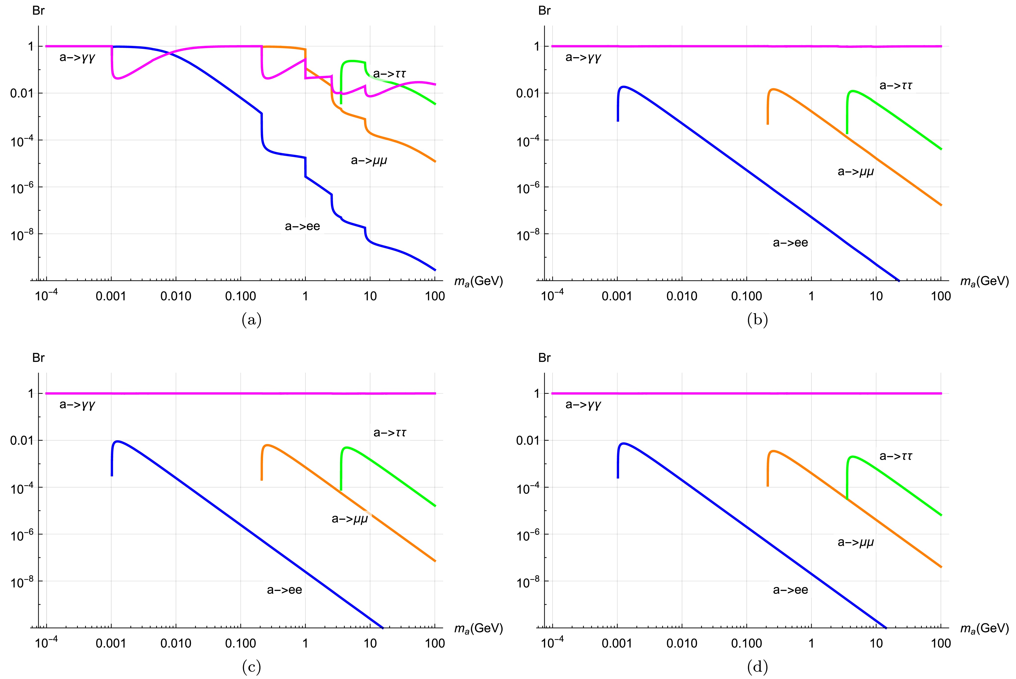

Figure 2.  (color online) ALP branching ratios decays into different SM final states. The decays into photons, electrons, muons, and tauons are shown in magenta, blue, orange, and green, respectively. (a) Photobic ALP $ g_{a\gamma\gamma}=0 $. (b) ALP with $ g_{aB}=0 $. (c) Same sign case $ g_{aB}=g_{aW}\tan^2\theta_W $. (d) ALP with $ g_{aW}=0 $.

By inputting the photophobic form in Eq. (45) into the above phenomenological physical processes and comparing it to the experimental observables in Table 2, we can obtain the corresponding exclusion parameter regions for $ m_a $ and $ g_{aW} $. The parameter bounds are plotted in Fig. 3(a). Here, we choose the ALP mass regions with $ 10^{-4}<m_a<100 $ GeV. The lower bound indicates $ m_a<2m_e $, and the upper bound represents the electroweak scale.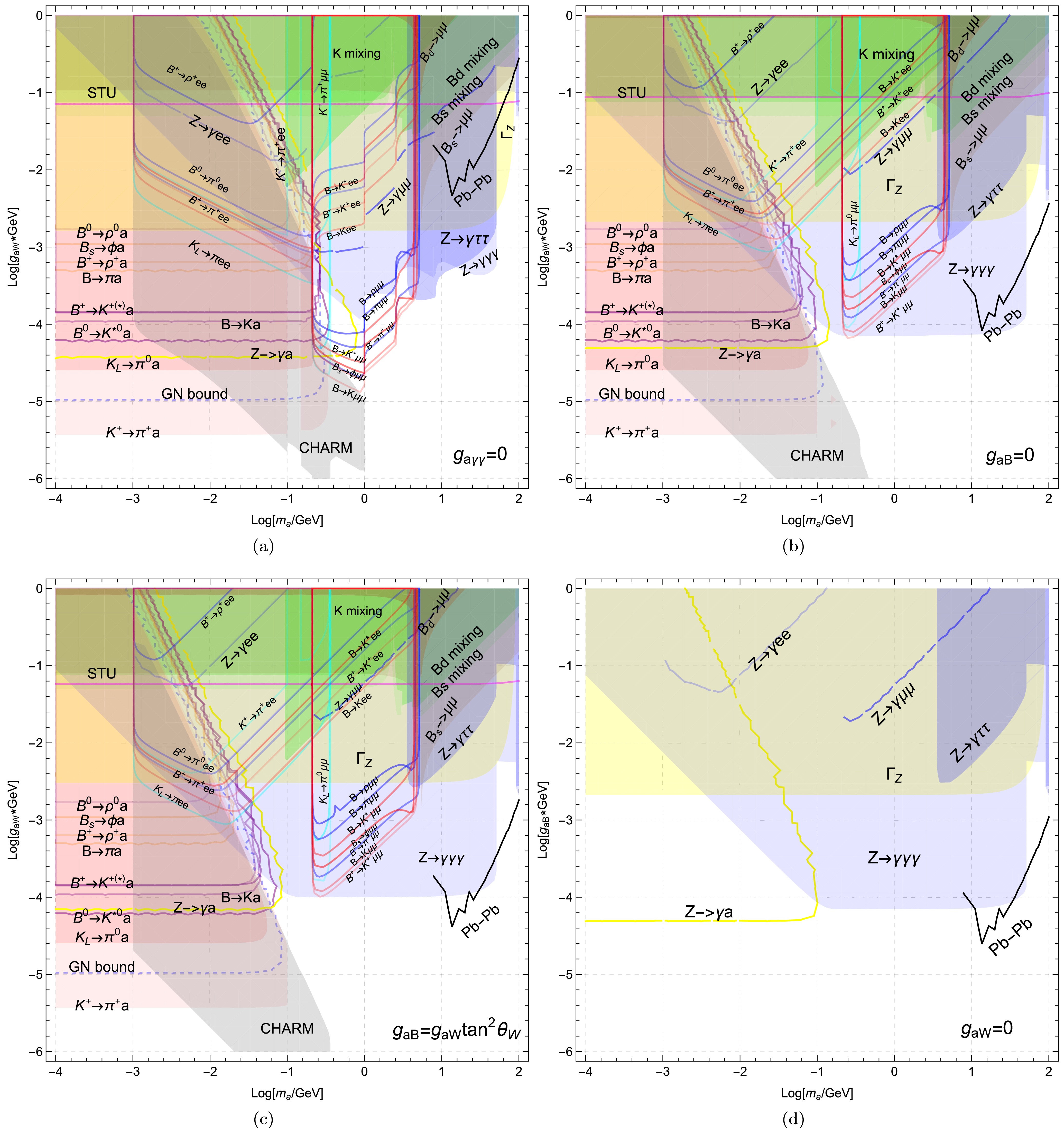

Figure 3.  (color online) Excluded parameter regions from different physical processes in the plane $ m_a-g_{aW} $ or $ m_a-g_{aB} $. The different physical processes exhibit distinctive exclusion capabilities, as shown in different colors. (a) Photobic ALP $ g_{a\gamma\gamma}=0 $. (b) ALP with $ g_{aB}=0 $. (c) Same sign case $ g_{aB}=g_{aW}\tan^2\theta_W $. (d) ALP with $ g_{aW}=0 $.

We found that different physical processes exhibit distinctive exclusion abilities, as shown in different colors. For three different quark transitions, $ s \to d $, $ b \to d $, and $ b \to s $, different decays demonstrate distinct exclusion capabilities. Note that the physical processes $ M_1 \to M_2 \nu\bar{\nu} $ should include the decay factor ($ 1 - {\cal{P}}_{{\rm{dec}}}^{a} $) to place the parameter constraints when ALP decays outside the detector.

For the $ s \to d $ quark transition, the most stringent bound comes from $ K^+ \to \pi^+ a $ with $ g_{aW} > 10^{-5.4} $ GeV^–1 in the mass region $ m_a < m_{K^+} - m_{\pi^+} $, which is stronger than $ K_L \to \pi^0 a $ by an order of magnitude. This implies that the NA62 experiment provides a comparable exclusive limit to the previous E949 experiment. The gap around $ m_a \in (100,150) $ MeV is caused by the pion mass pole from the NA62 Collaboration [39]. Additionally, the GN bound provides stronger constraints, especially in the mass gap region and for large $ g_{aW} $ shown in the blue dashed line. It approaches $ g_{aW} \sim 10^{-5} $ GeV^–1, providing considerably stronger constraints than $ K_L \to \pi a $, but weaker constraints than $ K^+ \to \pi^+ a $.

For the $ b \to d $ quark transition, $ B \to \pi a $ provides the most stringent bounds with $ g_{aW} < 10^{-3.3} $ GeV^–1 for $ m_a < 0.16 $ GeV. Correspondingly, the bound weakens as follows: $ B^+ \to \rho^+ a $ with $ g_{aW} < 10^{-3.2} $ GeV^–1, $ B_s \to \phi a $ with $ g_{aW} < 10^{-3} $ GeV^–1, and $ B^0 \to \rho a $ with $ g_{aW} < 10^{-2.8} $GeV^–1. Additionally, large couplings with $ g_{aW} > 10^{-2.6} $ results in a loss of distinguishable capability for $ b \to d $ processes.

For the $ b \to s $ quark transition, $ B^0 \to K^{0*} a $ provides the most stringent bounds with $ g_{aW} < 10^{-4.2} $ GeV^–1 for $ m_a < 4.5 $ GeV. The limiting capability decreases sequentially by a factor of 1.6 from $ B^0 \to K^{0*} a $, $ B \to K a $, to $ B^+ \to K^{+*} a $.

If $ m_a > 2m_l $, the semi-leptonic decay $ M_1 \to M_2 ll $ can occur kinematically. Therefore, the relevant decay processes can provide bounds on model parameters within reasonable regions, as shown in Fig. 3(a). For $ M_1 \to M_2 ee $, the strongest bounds come from $ K_L \to \pi ee $ within the oval for $ 0.001 < m_a < 0.1 $ GeV. The following bounds are from $ B \to K ee $, $ B^+ \to \pi^+ ee $, $ B^+ \to K^+ ee $, $ K^+ \to \pi^+ ee $, $ B^0 \to \pi^0 $, and $ B^+ \to \rho^+ $ within their respective circles. For $ M_1 \to M_2 \mu\mu $, $ B^+ \to K^+ \mu\mu $ excludes $ g_{aW}>10^{-4.8} $ GeV^–1, followed by $ B\to K\mu\mu $, $ B^+ \to \pi^+ \mu\mu $, $ B_s \to \phi \mu\mu $, $ B\to K^*\mu\mu $, $ B\to \pi\mu\mu $ , and $ B\to \rho\mu\mu $. Additionally, the upward-right tilt of the contour for $ M_1\to M_2 ll $ arises from the reduction in $ {\rm Br}(a\to ll) $, implying that larger values of the coupling $ g_{aW} $ are excluded by Eq. (26). These bounds effectively complement the unexplored regions for $ K^+ \to \pi^+ a $, particularly in the range $ 2m_l < m_a < m_{M_1}-m_{M_2} $.

Moreover, the purely leptonic decays $ B_{d/s} \to ll $ can provide the bounds shown in brown. Currently, experimental data indicate that muon final states impose stronger constraints than tauon cases. By analyzing $ B_{d/s} \to \mu\mu $, we find that $ B_d \to \mu\mu $ provides significantly weaker bounds than $ B_s \to \mu\mu $, around $ 10^{1.6} $ orders of magnitude, which constrains $ g_{aW} < 10^{-1} $ GeV^–1 at most mass ranges except $ m_a\sim m_{B_s} $. Additionally, the excluded regions by $ B_s \to \mu\mu $ fully encompass those by $ B_d \to \mu\mu $.

Similarly, neutral meson mixings provide bounds shown in green. $ B_s-\bar{B}_s $ mixing can place constraints across the ALP mass region with $ g_{aW} < 10^{-1.4} $ GeV^–1. $ B_d-\bar{B}_d $ mixing offers comparably weaker constraints. $ K-\bar{K} $ mixing can achieve $ g_{aW} \sim 10^{-2} $, which provides stronger bounds than $ B_s-\bar{B}_s $ mixing, especially for $ 0.1 < m_a < 1 $GeV. Additionally, while neutral meson mixings provide weaker constraints compared to rare meson decays, they exclude some unexplored regions for meson decays.

For the Z boson properties, the bounds from the Z boson decay chains are shown in yellow. $ \Gamma_Z $ excludes $ g_{aW} > 10^{-2.8} $ GeV^–1 across the ALP mass region. $ Z \to a\gamma $ can reach $ g_{aW} \sim 10^{-4.2} $and fill a small region between the yellow line and rare meson decays. Furthermore, the excluded region is fully covered by $ M_1\to M_2ll $ for $ m_a>2m_\mu $. Similarly, ALPs can decay into $ \gamma\gamma, ll $ to produce $ Z \to 3\gamma, \gamma ll $. The relevant bounds are shown in blue. $ Z \to \gamma ee $, $ Z \to \gamma \mu\mu $, and $ Z \to \gamma \tau\tau $ exclude regions within their respective capabilities. Moreover, $ Z \to 3\gamma $ provides the most stringent bounds, encompassing all $ Z \to \gamma ee, \mu\mu $ regions and a significant portion of $ Z \to \gamma\tau\tau $.

Besides, ultra-peripheral Pb-Pb collisions can produce ALPs through photon fusion, providing direct constraints on the ALP-photon coupling $ g_{a\gamma\gamma} $ in the mass range $ m_a=(5-100) $ GeV. These constraints are recast as a black solid line [90, 91]. We find that the bound from Pb-Pb collision is relatively weak and fully covered by other limits. Additionally, the Drell-Yan process $ pp \to \gamma a $ at the LHC can provide bounds for $ m_a > 100 $ GeV, as mentioned in Ref. [51], which is beyond the mass range of interest considered in our study.

Proton beam dump experiments searching for long-lived particles provide constraints complementary to those from direct searches for rare meson decays. Production occurs through rare decays $ K \to \pi a $ and $ B \to \pi/K a $, followed by the displaced decay $ a \to \gamma\gamma,ee,\mu\mu $ within the detector. The strongest bound is from the CHARM experiment [92], with the number of signals from ALP decays estimated in [45, 93].

where $ \gamma=10\;\rm{GeV}/m_a $. Since there is no signal from the CHARM experiment, one finds the 90% CL, $ N_{d}<2.3 $ [93]. The corresponding region is shown in gray in Fig. 3(a). We observe that the CHARM experiment sets very strong bounds on the coupling $ g_{aW} $. The CHARM shape exhibits three distinctive kick points, which correspond to the thresholds $ 2m_e $, $ 2m_\mu $ , and $ 3\pi $.

Therefore, we obtain the corresponding strongest bounds within the respective capability regions (shaded in gray).In the following, we analyze the future sensitivity for the ALP parameter regions.

First, we analyze the sensitivity of future lepton colliders for our model parameters. As indicated in Eq. (44), there is an enhancement factor $ m_Z^2/\Gamma_Z^2 $ relevant for future colliders operating at the Z pole energy $ \sqrt{s}=m_Z $. This highlights the importance of future lepton collider analyses at $ \sqrt{s}=m_Z $. Fortunately, based on the conceptual design, two $ e^+e^- $ colliders with $ \sqrt{s}=91 $ GeV exist, namely FCC-ee [94] and CEPC [95]. At this center-of-mass energy, the corresponding luminosities are 192 ab^-1 and 16 ab^-1, respectively, which implies that the sensitivity of future lepton colliders can be employed to constrain the parameter space. The corresponding cross-section is shown in Fig. 4(a). We found that for $ g_{aW}\sim 10^{-2} $, the cross-section approaches the $ \sigma(e^+e^-\to \gamma a)\sim (10^{-10}- 10^{-8}) $ barn depending on the ALP mass.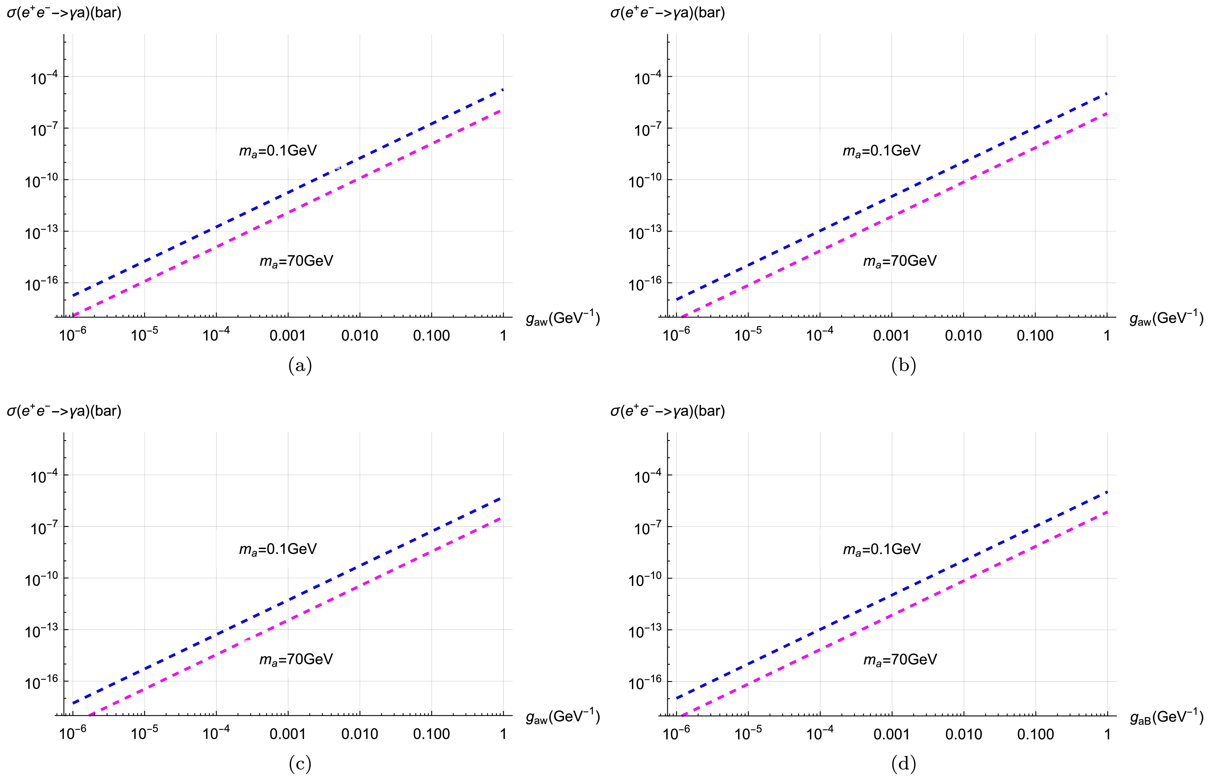

Figure 4.  (color online) Cross-section of $ e^+e^-\to \gamma a $ with the coupling $ g_{aW} $(GeV^–1) in the center of mass energy $ \sqrt{s}=m_Z $. Here, we illustrate two ALP mass choices, $ m_a=0.5 $ GeV and $ m_a=70 $ GeV. (a) Photobic ALP $ g_{a\gamma\gamma}=0 $. (b) ALP with $ g_{aB}=0 $. (c) Same sign case $ g_{aB}=g_{aW}\tan^2\theta_W $. (d) ALP with $ g_{aW}=0 $.

By further considering the decay of ALPs within the detector, we calculate the number of signal events as

where $ \ell_{lum} $ represents the luminosity of the lepton collider, and $ r(l_D) $ represents the minimal and maximal distances from the interaction point (IP) at which the detector can detect an ALP decay into SM particles. The main detector sensitivity is set as $ r=5 $ mm and $ l_D=1.22 $ mm [96]. Requiring $ N_{sig} \geq 3 $, we obtain the future sensitivity shown as a dashed line in Fig. 5(a), for CEPC and FCC-ee in magenta and orange, respectively. We find that FCC-ee provides better sensitivity than that of CEPC. Furthermore, FCC-ee can even reach $ g_{aW} \sim 10^{-7.4} $ GeV⁻¹ for $ m_a \sim 10^{1.6} $ GeV. Furthermore, the two colliders can cross-check the bounds from $ B\to K\mu\mu $. Additionally, FCC-ee and CEPC lose their discriminative capabilities for $ m_a>10^{-0.8} $ GeV and $ g_{aW}>10^{-5} $ GeV⁻¹.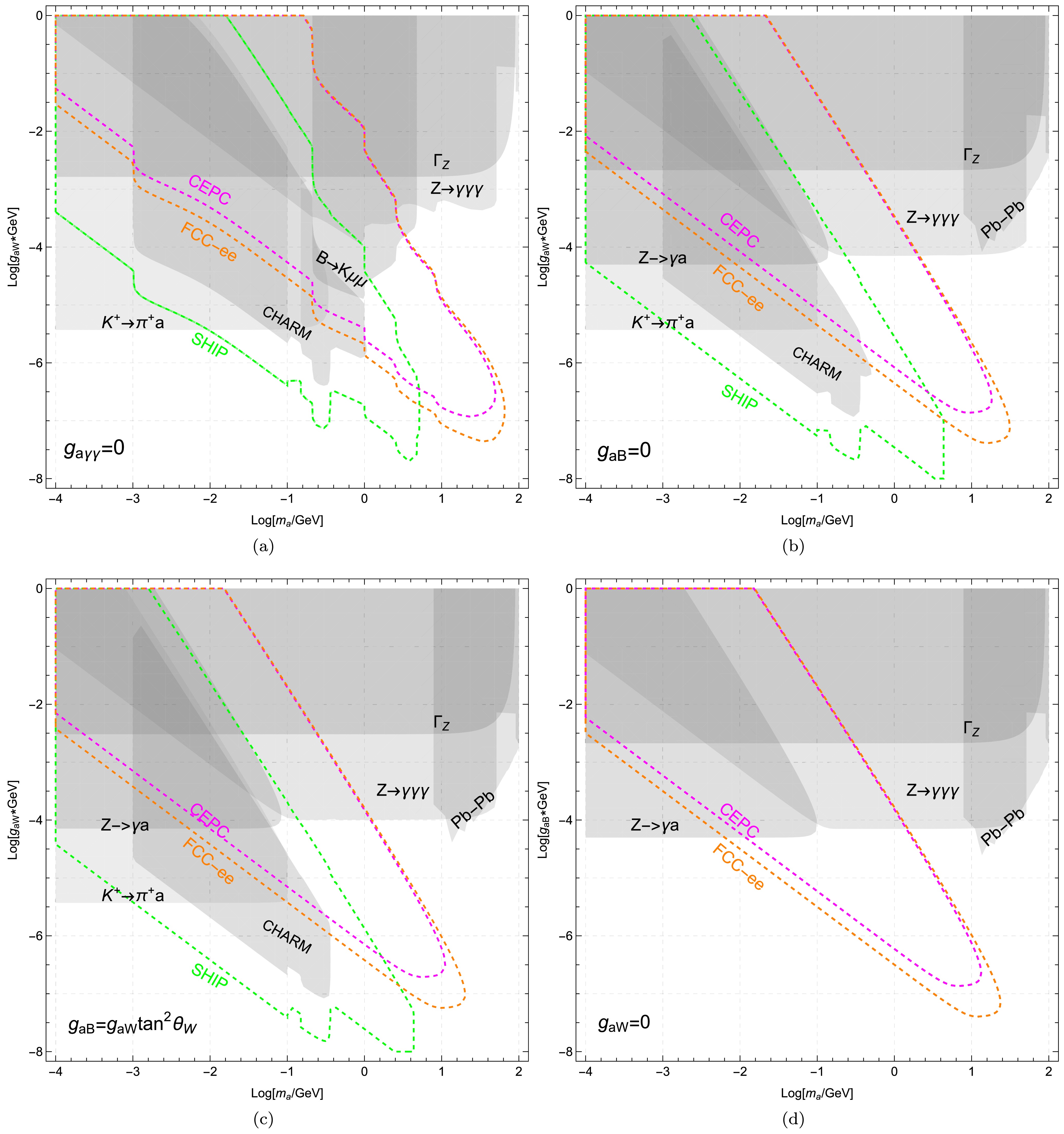

Figure 5.  (color online) Future sensitivity for the ALP parameter in the plane $ m_a-g_{aW} $ or $ m_a-g_{aB} $. The future sensitivity of lepton colliders (CEPC,FCC-ee) and SHiP are based on background-free assumptions, represented by magneta, orange, and green dashed lines, respectively. (a) Photobic ALP $ g_{a\gamma\gamma}=0 $. (b) ALP with $ g_{aB}=0 $. (c) Same sign case $ g_{aB}=g_{aW}\tan^2\theta_W $. (d) ALP with $ g_{aW}=0 $.

SHiP [97, 98] is an approved beam-dump experiment scheduled to begin operation in 2031. In SHiP, a 400 GeV proton beam extracted from the CERN SPS accelerator will impact a heavy proton target, resulting in significant production rates of pseudoscalar mesons $ K, B, B_s $. These produced mesons can be utilized to search for ALPs through rare meson decays. Assuming a nominal operation of 15 years yields $ 6\times 10^{20} $ protons on target, SHiP can produce total meson numbers of $ 1.71\times10^{20} $ for $ K $, $ 8.1\times10^{13} $ for $ B^{0,\pm} $, and $ 2.16\times10^{13} $ for $ B_s $ [99, 100]. Assuming these mesons decay into ALPs within the detector, which would lead to observable signals, we can obtain

where $ \gamma=25\;{\rm{GeV}}/m_a $, $ i=\pi, K, K^*, \rho $ and their corresponding charged components are considered. Adopting the latest design [98], the detector HSDS is located $ l=33 $ m downstream from the target with decay volume $ \Delta l=50 $ m. Similarly, requiring $ N_{sig} \geq 3 $, we obtain the future projection shown as a green dashed line in Fig. 5(a). We find that SHiP provides significant sensitivity, particularly for small $ g_{aW} $. Furthermore, the SHiP sensitivity projection completely encompasses the CHARM exclusion limits. Therefore, SHiP, CEPC, and FCC-ee serve as complementary explorations for ALPs, focusing on distinct parameter regions.

Note that the above sensitivity analysis assumes a background-free environment based on relatively clean experimental signatures. In practice, residual backgrounds including instrumental effects are expected, which would reduce detection sensitivity. This leads to detection efficiency degradation, requiring enhanced couplings $ g_{aW,aB} $. Consequently, the sensitivity regions shift upward. For simplicity, subsequent analysis focuses on the idealized background-free scenario.

Another interesting scenario is the ALP with $ g_{aB}=0 $, which couples only with $ S U(2)_L $ gauge bosons as

Correspondingly, the ALP interaction with fermions at the loop level is obtained as

Note that the tree-level $ g_{a\gamma\gamma} $ is significantly larger than the loop contribution $ g^{\rm loop}_{a\gamma\gamma} $ and $ g_{aFF} $ by approximately one order of magnitude. The associated branching ratios for ALP decay processes are drawn in Fig. 2(b). We find that regardless of the ALP mass, the dominant decay channel is $ a \to \gamma\gamma $ with a branching ratio close to 1. Additionally, chains decaying into charged leptons are strongly suppressed even if kinematically allowed. This feature differs significantly from the photophobic case, which suggests that different parameter bounds could exist in the ALP scenario with $ g_{aB}=0 $.

Similarly, using Eq. (49) to analyze physical processes and comparing them with the experimental observables in Table 2, the corresponding exclusion parameter regions for $ g_{aW} $ are shown in Fig. 3(b) for $ 10^{-4} < m_a < 100 $ GeV.

The different physical processes show distinct exclusion abilities represented by different colors. We find that the largest upper bound for $ g_{aW} $ maintains the same constraints as that in the photophobic ALP scenario. However, the corresponding excluded regions are narrowed because of the enhanced total decay width, which affects the decay factor ($ 1-{\cal{P}}_{{\rm{dec}}}^{a} $).

For rare meson two-body decays $ M_1 \to M_2 a $, three different quark transitions — $ s \to d $, $ b \to d $, and $ b \to s $ — move left as the coupling $ g_{aW} $ increases. For instance, when $ g_{aW} = 1 $ GeV^–1, the excluded mass changes from $ 10^{-2.2} $ GeV in the photophobic scenario to $ 10^{-3} $ GeV. For the $ s \to d $ quark transition, the lowest excluded value remains consistent with the photophobic case at $ g_{aW} \sim 10^{-5.4} $ GeV^–1. Note that the original gap around the pion mass disappears because the weakened exclusion capability constrains $ m_a < 10^{-1} $ GeV. The excluded regions by the GN bound lie between $ K_L \to \pi^0 a $ and $ K^+ \to \pi^+ a $. Both reduce correspondingly to $ m_a < 10^{-1} $ GeV. Similarly, the constrained ALP mass decreases from $ 10^{-0.6} $ GeV to $ 10^{-1} $ GeV for $ b \to s $ quark transition, and from $ 10^{-0.8} $ GeV to $ 10^{-1.6} $ GeV for $ b \to d $ quark transition. Correspondingly, the bound ability weakens similarly to the photophobic scenario, followed by $ B \to \pi a $, $ B^+ \to \rho^+ a $, $ B_s \to \phi a $, and $ B^0 \to \rho a $ for the $ b \to d $ transition. The limiting capability decreases sequentially from $ B^0 \to K^{0*} a $, $ B \to K a $ to $ B^+ \to K^{+(*)} a $ for the $ b \to s $ transition. Additionally, the exclusion capability becomes indistinguishable for large coupling $ g_{aW} $.

For the semi-leptonic decay $ M_1 \to M_2 ll $, the constraints weaken when kinematically allowed decays occur. The bounded regions are illustrated in Fig. 3(b). For the electron case, the bounded circle shifts to the upper left panel, which corresponds to $ g_{aW} \sim 10^{-3} $, as given by $ K_L \to \pi ee $. The subsequent bounds are derived from $ B \to K ee $, $ B \to K^* ee $, $ B^+ \to K^+ ee $, $ B^+ \to \pi^+ ee $, $ B \to K^* ee $, $ K^+ \to \pi^+ ee $, $ B^0 \to \pi^0 $, and $ B^+ \to \rho^+ $, each showing varying degrees of weakening. For muon cases, the corresponding bounds shift upward, indicating that $ M_1 \to M_2 ll $ impose weaker bounds on the model parameters, reduced by an order of magnitude of $ 10^{-0.6} $ compared to that of the photophobic case.

For pure leptonic decays $ B_{d/s} \to ll $, the bounds remain approximately the same in brown with the photophobic case because of minor modifications in $ g_{aFF} $. The $ B_s \to \mu\mu $ excluded region fully encompasses the ones by $ B_d \to \mu\mu $ with a decreased $ g_{aW} $. Additionally, neutral meson mixings remain unchanged as the process solely depends on the coupling $ g_{ad_i d_j} $ induced by $ g_{aW} $.

For the Z boson properties, the bounds from the Z boson invisible decays increase slightly because of the modification $ g_{a\gamma Z} $ from $ 2\tan\theta_W g_{aW} $ to $ 2c_W s_W g_{aW} $, as shown in yellow. In addition, $ Z \to a\gamma $ restricted interval decreases from $ m_a \sim 10^{-0.2} $ GeV to $ m_a \sim 10^{-0.8} $ GeV, indicating that the excluded regions do not intersect with $ M_1\to M_2 \mu\mu $. This feature is obviously different from the photophobic scenario, which helps explore small regions in previously unexplored meson decays. Furthermore, the exclusion capability of $ Z \to \gamma ll $ weakens to varying degrees. For instance, $ Z \to \gamma\tau\tau $ constrains $ g_{aW} < 10^{-2.8} $ GeV^–1, which is weaker than the previous bound $ g_{aW} < 10^{-3.4} $ GeV^–1 in the photophobic case. However, the enhanced decay ratio $ a \to \gamma\gamma $ strengthens the corresponding bounds to around $ g_{aW} < 10^{-4.2} $ GeV^–1 for $ m_a \in (10^{-1}, 10^{1.6}) $ GeV. Furthermore, $ Z \to 3\gamma $ covers all regions excluded by $ Z \to \gamma ll $.

The Pb-Pb collision constraint is displayed as a black solid line, which provides the most stringent constraints in the ALP mass range $ m_a=(91,100) $ GeV.

Proton beam dump experiments (CHARM) have already excluded some regions in gray with a corresponding leftward shift. The excluded region by CHARM covers all coupling ranges $ g_{aW} \in (10^{-6}, 1) $ GeV^–1. In the following, we analyze the future sensitivity for ALP parameter regions.

For the future lepton collider (CEPC, FCC-ee) operating at the Z pole with $ \sqrt{s} = m_Z $, the corresponding cross-section is shown in Fig. 4(b). We observe that the cross-section only undergoes minor modifications. For example, $ \sigma(e^+e^-\to \gamma a) \sim 10^{-7} $ bar for $ m_a = 0.1 $ GeV and $ g_{aW} = 0.1 $ GeV^–1.

After analyzing the ALP decay within the detector and requiring the signal events to be larger than 3, we obtain the future sensitivity shown as a dashed line in Fig. 5(b), for CEPC and FCC-ee in magenta and orange, respectively. FCC-ee can provide significantly better sensitivity than CEPC. By contrast, SHiP can produce a large number of pseudoscalar mesons decaying into ALP with the sensitivity shown as a green dashed line. Therefore, SHiP can provide strong sensitivity, especially for small $ g_{aW} $. This shows that they can serve as complementary explorations for ALP, focusing on different parameter regions, respectively.

Instead of selecting the opposite-sign coupling $ g_{aB}=-g_{aW}\tan^2\theta_W $ to cancel out $ g_{a\gamma\gamma} $ in the photophobic scenario, we adopt the same-sign coupling $ g_{aB}= g_{aW}\tan^2\theta_W $ to enhance $ g_{a\gamma\gamma} $. We defined the case as a same sign ALP scenario with

Correspondingly, the ALP interaction with fermions at the loop level is obtained as

Note that the tree-level $ g_{a\gamma\gamma} $ is four times larger compared to the ALP scenario with $ g_{aB}=0 $, and it is further significantly larger than both the loop contribution $ g^{\rm loop}_{a\gamma\gamma} $ and $ g_{aFF} $. The associated branching ratios for ALP decay processes are drawn in Fig. 2(c), indicating that the dominant decay channel is $ {\rm Br}(a \to \gamma\gamma)\sim 1 $across the entire ALP mass range. Additionally, the decay into charged leptons is strongly suppressed, with ratios below 0.01. This feature is similar to the $ g_{aB}=0 $ scenario, which yields similar parameter bounds.

By leveraging Eq. (51) to analyze physical processes and comparing it with experimental observables in Table 2, the corresponding exclusion parameter regions for $ g_{aW} $ are shown in Fig. 3(c) for $ 10^{-4} < m_a < 100 $ GeV.

The different physical processes show distinct exclusion abilities represented by different colors. We find that bounds from meson decays, including $ M_1\to M_2 a $, $ M_1\to M_2 ll $, and $ M_1\to ll $, have similar constraints to those in the ALP scenario with $ g_{aB}=0 $. This is because of the loop-suppressed ALP couplings with fermions and photons, which results in $ a\to \gamma\gamma $ being the dominant decay channel from the tree-level $ g_{a\gamma\gamma} $.

Additionally, the other bounds maintain comparable exclusion capabilities such as meson mixing and CHARM. The only significant changes involve Z boson-related processes. For the total decay width of the Z boson, the exclusion bound is modified to $ g_{aW}<10^{-2.6} $, improved from $ g_{aW}<10^{-2.8} $ in the $ g_{aB}=0 $ scenarios as shown in yellow. Furthermore, the $ Z \to a\gamma $ restricted interval decreases from $ m_a \sim 10^{-0.8} $ GeV to $ m_a \sim 10^{-1.2} $ GeV, which adds to previously unexplored rare meson decays. In addition, the exclusion capability of $ Z \to \gamma ll $ weakens to varying degrees as shown in blue. For example, $ Z \to \gamma\tau\tau $ constrains $ g_{aW} < 10^{-2.6} $ GeV^–1, which matches the exclusion capability of $ \Gamma_Z $. Correspondingly, $ a \to \gamma\gamma $ weakens the corresponding bounds to around $ g_{aW} < 10^{-4} $ GeV^–1 for $ m_a \in (10^{0.4}, 10^{1.6}) $ GeV. Furthermore, $ Z \to 3\gamma $ covers all regions excluded by $ Z \to \gamma ll $, even including the regions excluded by $ \Gamma_Z $. This feature differs slightly from the $ g_{aB}=0 $ scenario. Moreover, the bounds from Pb-Pb collisions in the black line are stringent for ALP masses in the range 10−100 GeV.

In the following, we analyze the future sensitivity for ALP parameter regions. For the future lepton collider (CEPC, FCC-ee) operating at the Z pole with $ \sqrt{s} = m_Z $, the corresponding cross-section is shown in Fig. 4(c), which maintains approximately the same cross-section.

Similarly, by analyzing the ALP decay within the detector and requiring the signal events to be greater than 3, we obtain the future sensitivity shown as a dashed line in Fig. 5(c) for CEPC and FCC-ee in magenta and orange, respectively. We find that the sensitivity shifts to the left, and the FCC-ee sensitivity can fully cover the CEPC sensitivity. SHiP sensitivity follows a similar trend of shifting to the left, providing strong sensitivity for a small $ m_a<4 $ GeV.

Correspondingly, another left ALP scenario is $ g_{aW}=0 $, which only couples with the $ U(1)_B $ hypercharge gauge boson as

Similarly, the ALP interaction with fermions at loop level is obtained as

Note that the tree-level $ g_{a\gamma\gamma} $ remains significantly larger than both loop contributions $ g^{\rm loop}_{a\gamma\gamma} $ and $ g_{aFF} $. The associated branching ratios for ALP decay processes are drawn in Fig. 2(d), demonstrating that the dominant decay channel is $ {\rm Br}(a \to \gamma\gamma)\sim 1 $ across the entire ALP mass range. Furthermore, the decay branching ratios into charged leptons are significantly suppressed to below 0.01. This feature is consistent with that in the other scenarios, which yield similar parameter constraints.

Using Eq. (53) to analyze physical processes and compare with the experimental observables in Table 2, the corresponding exclusion parameter regions for $ g_{aW} $ are presented in Fig. 3(c) for $ 10^{-4} < m_a < 100 $ GeV. Different physical processes exhibit distinct exclusion capabilities, represented by various colors. For $ g_{aW}=0 $, the flavor changing interactions in Eq. (12) vanish, causing the relevant bounds ($ M_1\to M_2 a $, $ M_1\to M_2 ll $ and meson mixings) to disappear. The only remaining physical processes are Z boson-related interactions. For $ m_a<0.1 $ GeV, the strongest bounds originate from $ {\rm Br}(Z\to \gamma a) $ with $ g_{aB}<10^{-4.3} $ GeV^–1. For $ m_a>0.1 $ GeV, the stringent constraint arises from $ Z\to 3\gamma $ with $ g_{aB}<10^{-4.2} $ GeV^–1. Other subsequent decays such as $ Z\to all $ provide relatively weak constraints, which are entirely covered by the total decay width of the Z boson $ \Gamma_Z $, as indicated in yellow. Additionally, the Pb-Pb collision constraints in black solid line dominate over Z-boson decay limits across most of the parameter space for $ m_a=(10,100) $ GeV.

For the future sensitivity of ALP parameter regions, the projected performance of future lepton colliders (e.g., CEPC and FCC-ee) operating at the Z pole ($ \sqrt{s} = m_Z $) is shown in Fig. 4(d). Similarly, by analyzing ALP decays within the detector and requiring at least three signal events, we derive the projected future sensitivity shown as dashed lines in Fig. 5(d), with CEPC and FCC-ee in magenta and orange, respectively. We find that FCC-ee offers significantly better sensitivity compared to that of CEPC. Additionally, they can act as complementary probes for ALPs, in comparison to Z boson decays.

We provide an updated and extended analysis on the experimental limits of the ALP couplings to electroweak gauge bosons across the ALP mass range from MeV to 100 GeV. To indicate the effects from two independent couplings ($ g_{aW} $ and $ g_{aB} $), we analyze four distinct scenarios under various values of couplings. The couplings induce flavor-conserving ALP interactions with SM fermions at the one-loop level, while $ g_{aW} $ additionally induce flavor-changing ALP-quark couplings within the framework of minimal flavor violation.

The relevant experimental constraints are illustrated in Fig. 3. We clearly depict the bounds from each different physical process. This helps us identify which process contributes to which specific constraint. For the three quark transition scenarios $ s \to d $, $ b \to d $, and $ b \to s $, the strongest bounds are provided by $ K^+ \to \pi^+ a $, $ B \to \pi a $, and $ B^0 \to K^{0*} a $, respectively. With more precise future measurements of certain processes, we will be able to understand how the constraints on the parameter space evolve. Comparing these four different scenarios ($ g_{a\gamma\gamma}=0 $, $ g_{aB}=0 $, $ g_{aB}=g_{aW}\tan^2\theta_W $ and $ g_{aW}=0 $), we find that the excluded region in the photophobic case is significantly weaker than that in the other three cases because of the enhanced photon coupling at the tree level for the latter. The corresponding excluded regions shift to the left panel for these four scenarios along with the increased total ALP decay width. Another distinct difference is that the bounds from $ M_1 \to M_2 ll $ move up as the scenario transitions from photophobic and $ g_{aB}=0 $ ALPs to same-sign ALPs, and even vanish in the ALPs with $ g_{aW}=0 $, indicating a gradual weakening of constraints. Furthermore, $ Z \to 3\gamma $ in the last three scenario provides considerably stricter bounds than that in the photophobic ALP case because of the enhanced branching ratio $ a \to \gamma\gamma $. Additionally, Pb-Pb collisions provide stringent constraints in $ m_a=(1,100) $ GeV. Our finding highlights that rare meson decays, Z-boson decays, and Pb-Pb collisions provide complementary probes of ALP parameter space, covering MeV and GeV mass scales.

The future experimental projections for ALP parameters are analyzed as shown in Fig. 5, including lepton colliders (CEPC, FCC-ee) and SHiP. For lepton colliders operating near the Z pole, the ALP production via $ e^+e^-\to Z\to \gamma a $ experiences an enhancement factor of $ m_Z^2/\Gamma_Z^2= $ 1330, requiring an analysis of the corresponding projection. We find that FCC-ee can provide better sensitivity than that of CEPC, which enables probing regions beyond the bounds from rare meson decays and Z-boson decays. Moreover, SHiP can explore deeper into smaller $ g_{aW} $ values, fully surpassing the existing CHARM bounds. These results indicate that future lepton colliders and SHiP can offer enhanced sensitivity for ALP parameters.

We thank Prof. YuJi Shi and Prof. Sang Hui Im for the useful discussions.