Mass mixing between QCD axions

QCD axions are attractive candidates for cold dark matter (DM). The canonical QCD axion was predicted by the Peccei-Quinn (PQ) mechanism [1, 2] to solve the strong CP problem in the Standard Model (SM) [3–8]. It obtains a tiny mass from the QCD non-perturbative effects [9, 10]. As a DM candidate, it can be non-thermally produced in the early Universe through the misalignment mechanism [11–13]. At high cosmic temperatures, the QCD axion is massless and obtains a non-zero mass during the QCD phase transition. The oscillation of the axion when its mass is comparable to the Hubble parameter explains the observed DM abundance. See, $ { {e.g.}} $, Ref. [14] for a recent review. The reduced-mass $ Z_{{\cal{N}}} $ axion [15] can also solve the strong CP problem with $ {\cal{N\geqslant}}3 $ [16] and account for DM through the trapped plus kinetic misalignment mechanism [17, 18]. Here, $ {\cal{N}} $ is an odd number, and $ {\cal{N}} $ mirror worlds that are nonlinearly realized by the axion field under a $ Z_{{\cal{N}}} $ symmetry can coexist in nature. Due to the suppressed non-perturbative effects on axion potential from the $ {\cal{N}} $ degenerate QCD groups, the $ Z_{{\cal{N}}} $ axion mass is exponentially suppressed at the QCD phase transition. To avoid confusion, in what follows, "QCD axion" only represents the canonical QCD axion.

The mass mixing in the multiple axions model [19] has attracted extensive attention in recent years. ¹ Considering the non-zero mass mixing between these axions, the cosmological evolution process of the mass eigenvalues, called the level crossing, can occur and induce the adiabatic transition of the axion energy density, which is similar to the MSW effect [23–25] in neutrino oscillations. The level crossing has some interesting cosmological implications, such as the modification of the axion relic density and isocurvature perturbations [26–29], domain wall formation [30], gravitational wave emission and primordial black hole formation [31–33], and dark energy composition [34, 35].

In this study, we investigate the mass mixing between QCD axions: one QCD axion and one $ Z_{{\cal{N}}} $ axion. We find that level crossing can occur at the QCD phase transition critical temperature or slightly before it, depending on the relationship between the axion decay constants. The conditions for level crossing to occur in these two cases are discussed in detail. The cosmological evolution of the mass eigenvalues in both cases is similar, whereas the transition of energy density among the axions differs. Finally, we estimate the relic density of the QCD axion and $ Z_{{\cal{N}}} $ axion DM through the misalignment mechanism. To the best of our knowledge, this is the first investigation of the effect of level crossing in the mass mixing within a multiple QCD axions model.

Here, we consider a minimal multiple QCD axion model, with one QCD axion ϕ and one $ Z_{{\cal{N}}} $ axion φ. These two axions are charged under two copies of the SM, yet both are coupled to QCD. We expect ϕ to receive the dominant contribution from the QCD potential, leading to the cancellation of the potential that occurs in the usual $ Z_{{\cal{N}}} $ axion case, while such cancellation would not occur for the single φ. ² The low-energy effective Lagrangian is given by

where $ m_a(T) $ and $ m_{{\cal{N}}}(T) $ are the temperature-dependent QCD axion and $ Z_{{\cal{N}}} $ axion masses, respectively, and $ f_a $ and $ F_a $ are the QCD axion and $ Z_{{\cal{N}}} $ axion decay constants, respectively. The QCD axion mass $ m_a(T) $ can be described by

where $ m_\pi $ and $ f_\pi $ represent the mass and decay constant of the pion, respectively, $ z\equiv m_u/m_d\simeq 0.48 $ signifies the ratio of the up to down quark masses, $ T_{{\rm{QCD}}}\simeq 150\; {\rm{MeV}} $ is the QCD phase transition critical temperature, and $ b\simeq 4.08 $ is an index taken from the dilute instanton gas approximation. The first term in Eq. (2) corresponds to the zero-temperature QCD axion mass $ m_{a,0} $. The $ Z_{{\cal{N}}} $ axion mass $ m_{{\cal{N}}}(T) $ can be described by

where $ \gamma\in(0,1) $ is a temperature parameter. The first term in Eq. (3) also corresponds to the zero-temperature $ Z_{{\cal{N}}} $ axion mass $ m_{{{\cal{N}}},0} $. Notably, this mass undergoes a sudden exponential suppression at $ T_{{\rm{QCD}}} $ due to the $ Z_{{\cal{N}}} $ symmetry. Subsequently, the equations of motion of ϕ and φ are given by

and

where $ H(T) $ is the Hubble parameter, and the dots represent derivatives with respect to physical time t. By diagonalizing the mass mixing matrix

we can derive the heavy ($ a_h $) and light ($ a_l $) axion mass eigenstates

with the corresponding mass eigenvalues $ m_{h,l}(T) $

where α is the mass mixing angle

The so-called axion level crossing occurs when, considering the interaction between two axion fields, there exists a nontrivial mass mixing of their temperature-dependent mass eigenvalues $ m_{h,l}(T) $ that is a function of the cosmic temperature T. This can occur when the difference of $ m_h^2(T)-m_l^2(T) $ is minimized.

We first consider a case where the zero-temperature QCD axion mass $ m_{a,0} $ is smaller than the second term in Eq. (3) (we can define this as the mass $ m_{{{\cal{N}}},\pi} $)

which can be characterized as

where we have defined the ratio ζ. Meanwhile, for level crossing to occur in this case, the zero-temperature QCD axion mass should be larger than the zero-temperature $ Z_{{\cal{N}}} $ axion mass $ m_{{{\cal{N}}},0} $, i.e.,

which can also be characterized as

which depends on the value of $ {\cal{N}} $. Fig. 1 (left) illustrates level crossing in this case. We have set $ f_a=10^{12}\;{{\rm{GeV}}} $, $ F_a=10^{11.5}\,{{\rm{GeV}}} $, $ {\cal{N}}=17 $, and $ \gamma=0.25 $. The red and blue lines correspond to the temperature-dependent mass eigenvalues $ m_h(T) $ and $ m_l(T) $, respectively. Note that the level crossing occurs at the QCD phase transition critical temperature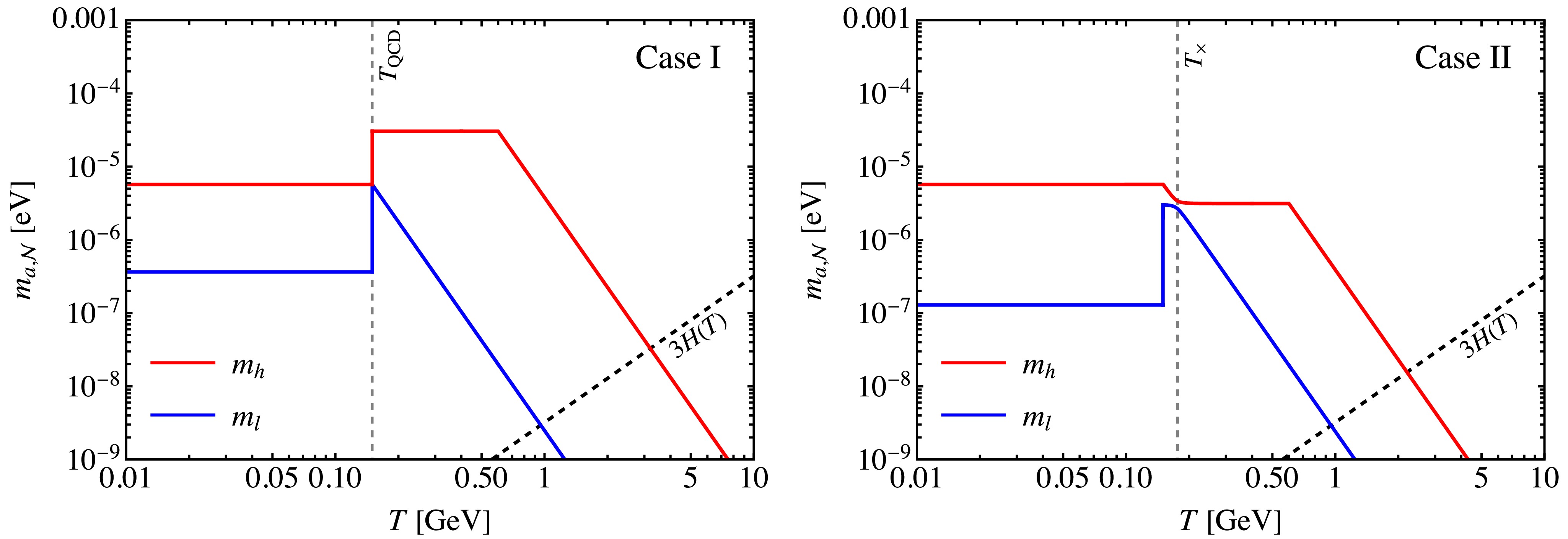

Figure 1.  (color online) Illustrations of level crossing in Cases I (left) and II (right). The red and blue lines represent the mass eigenvalues $ m_h(T) $ and $ m_l(T) $, respectively. The black dashed line represents the Hubble parameter $ H(T) $. Left: We set $ f_a=10^{12}\,{{\rm{GeV}}} $, $ F_a=10^{11.5}\,{{\rm{GeV}}} $ ($ \Rightarrow \zeta\simeq 0.32 $), $ {\cal{N}}=17 $, and $ \gamma=0.25 $. The gray dashed line represents the temperature $ T_{{\rm{QCD}}} $. Right: We set $ f_a=10^{12}\,{{\rm{GeV}}} $, $ F_a=10^{12.5}\,{{\rm{GeV}}} $ ($ \Rightarrow \zeta\simeq 3.16 $), $ {\cal{N}}=13 $, and $ \gamma=0.25 $. The gray dashed line represents the level crossing temperature $ T_\times\simeq 176.3\, {\rm{MeV}} $.

Here, we discuss the cosmological evolution of the mass eigenvalues in this scenario. At high temperatures, the heavy mass eigenvalue $ m_h(T) $ corresponds to the $ Z_{{\cal{N}}} $ axion, whereas the light one $ m_l(T) $ corresponds to the QCD axion. They will approach each other at $ T_{{\rm{QCD}}} $ and then move away from each other. When $ T < T_{{\rm{QCD}}} $, $ m_h(T) $ represents the QCD axion, and $ m_l(T) $ represents the $ Z_{{\cal{N}}} $ axion. For a more intuitive description, we can express them as follows:

and

The above discussion is focused on Case I, where level crossing occurs at $ T_{{\rm{QCD}}} $.

To compare with another case discussed below, we show the condition for level crossing to occur in Case I by using Eqs. (11) and (13). See Fig. 2 with the red shaded region in the $ \{{{\cal{N}}}, \, \zeta\} $ plane. The unshaded regions represent areas where no level crossing occurs.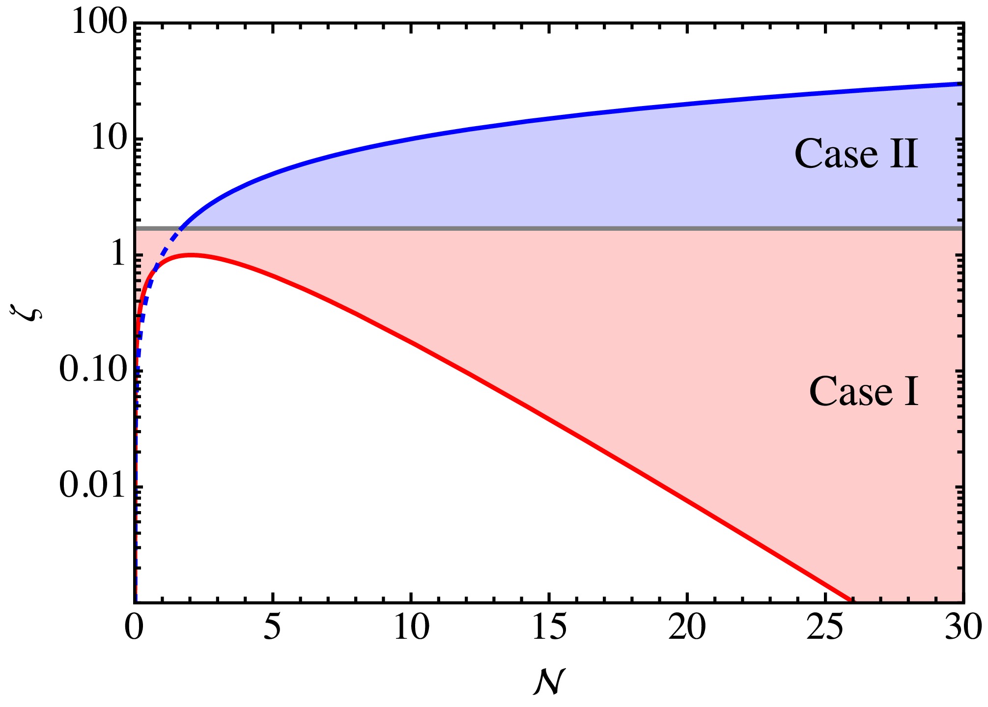

Figure 2.  (color online) Conditions for level crossing to occur in the $ \{{{\cal{N}}}, \, \zeta\} $ plane. The red and blue shaded regions correspond to Cases I and II, respectively. The gray line represents $ \zeta=1.69 $. Note that $ {{\cal{N}}}=2k+1 $, $ k\in\mathbb{N}^+ $.

Next, we consider the case where the zero-temperature QCD axion mass is larger than $ m_{{{\cal{N}}},\pi} $. We have

We present an illustration of this case in Fig. 1 (right). We have set $ f_a=10^{12}\,{{\rm{GeV}}} $, $ F_a=10^{12.5}\,{{\rm{GeV}}} $, $ {\cal{N}}=13 $, and $ \gamma=0.25 $. Here, in contrast to that in Case I, the level crossing takes place slightly before the temperature $ T_{{\rm{QCD}}} $. By solving $ {\rm d}(m_h^2(T)-m_l^2(T))/{\rm d}T=0 $ at $ T_{{\rm{QCD}}} < T < T_{{\rm{QCD}}}/\gamma $, we obtain the level crossing temperature

which is slightly higher than $ T_{{\rm{QCD}}} $. The QCD axion mass at $ T_\times $ is given by

Note that the condition $ \zeta<{\cal{N}} $ should be satisfied in Eq. (18). This level crossing persists for a parametric duration given by

where $ \alpha(T) $ represents the mass mixing angle given by Eq. (9). This scenario is referred to as Case II. The temperature-dependent behavior of the mass eigenvalues is similar to that in Case I. However, the transition of energy density between them differs significantly, as will be discussed in detail later. It is worth noting that Case I can transition into Case II, depending on the value of the ratio $ \zeta\sim 1.69 $.

Then, in Fig. 2 (blue shaded region), we illustrate the condition for level crossing to occur in Case II, using Eq. (17) and the inequality $ \zeta<{\cal{N}} $. Additionally, we note that at $ T_{{\rm{QCD}}}/\gamma $, the QCD axion mass should be smaller than the $ Z_{{\cal{N}}} $ axion mass

which can be characterized as

which depends on the value of γ. For the small γ, the constraint of $ \zeta<{\cal{N}} $ is more stringent than Eq. (22). Thus, we do not include it in Fig. 2.

Here, we estimate the relic density of the axion DM in Cases I and II through the misalignment mechanism. We consider the pre-inflationary scenario, in which the PQ symmetry is spontaneously broken during inflation.

We first discuss Case I, focusing on the $ Z_{{\cal{N}}} $ axion DM. ³ We begin with the QCD axion field, which is frozen at high temperatures with an arbitrary initial misalignment angle $ \theta_{1,a} $ and starts to oscillate at $ T_{1,a} $. The oscillation temperature $ T_1 $ is given by $ m(T)=3H(T) $. In the following, the subscript "x" stands for the physical quantity at $ T_x $ or corresponding to x. The initial energy density in the QCD axion field is given by

At $ T_{{\rm{QCD}}}<T<T_{1,a} $, the QCD axion energy density is adiabatic invariant with the comoving number $ N_a \equiv \rho_a a^3 /m_a $, where a is the scale factor. Then, we have the QCD axion energy density just before $ T_{{\rm{QCD}}} $ as

In this case, the axion is trapped around $ \theta_{{\rm{tr}}}\equiv\theta_a(T_{{\rm{QCD}}}) $ until $ T_{{\rm{QCD}}} $, with the initial axion velocity $ \dot{\theta}_{{\rm{tr}}}\equiv\dot{\theta}_a(T_{{\rm{QCD}}}) $. At $ T=T_{{\rm{QCD}}} $, the light mass eigenvalue $ m_l(T) $ will comprise the $ Z_{{\cal{N}}} $ axion, the axion mass is suddenly suppressed, and the true minimum develops. Then, we have the mean velocity of the $ Z_{{\cal{N}}} $ axion

Note that the $ Z_{{\cal{N}}} $ axion energy density at $ T_{{\rm{QCD}}} $ is non-adiabatic, which just after $ T_{{\rm{QCD}}} $ is given by

where we consider a case that the axion has a large mean velocity. Then, the $ Z_{{\cal{N}}} $ axion will start to oscillate at $ T_2 $, which is defined as the temperature when the kinetic energy is equal to the barrier height. At $ T_2<T<T_{{\rm{QCD}}} $, the $ Z_{{\cal{N}}} $ axion energy density is conserved with the comoving PQ charge $ q_{{\rm{kin}}}=\dot{\theta}_{{\cal{N}}} a^3 $, and we have the scale factor at $ T_2 $ as $ a_2=({{\cal{N}}}\dot{\theta}_{{\rm{tr}}}/(2m_{{\cal{N}}}))^{1/3}a_{{\rm{QCD}}} $. Then, at $ T_0<T<T_2 $, the adiabatic approximation is valid, and we have the $ Z_{{\cal{N}}} $ axion energy density at present $ T_0 $ as

Substituting the mean velocity, it reads

where $ C\simeq 2 $ is a constant. Compared with the no mixing case, the relic density can be modified by

Then, in the left panel of Fig. 3, we show the distribution of $ R_{\rho} $ in the $ \{\zeta, \log(\eta)\} $ plane, where $ \eta \equiv m_{{{\cal{N}}},1}/m_{a,1} $ and the initial misalignment angles are assumed to be of order one. Considering the significant impact of the temperature parameter γ on the oscillation temperature of the $ Z_{{\cal{N}}} $ axion, we incorporate the variations in γ into the observed changes in η to provide a more intuitive illustration of how the relic density varies across different parametric conditions. We find that the ratio $ R_{\rho} $ is enhanced in most regions, whereas it is suppressed in a small subset of regions. Note that, in Case I, the parameter $ {{\cal{N}}} $ also exhibits a significant property related to ζ, as illustrated in Fig. 2. However, this property cannot be directly observed from Fig. 3, and here, we roughly set $ 0<\zeta<1.69 $.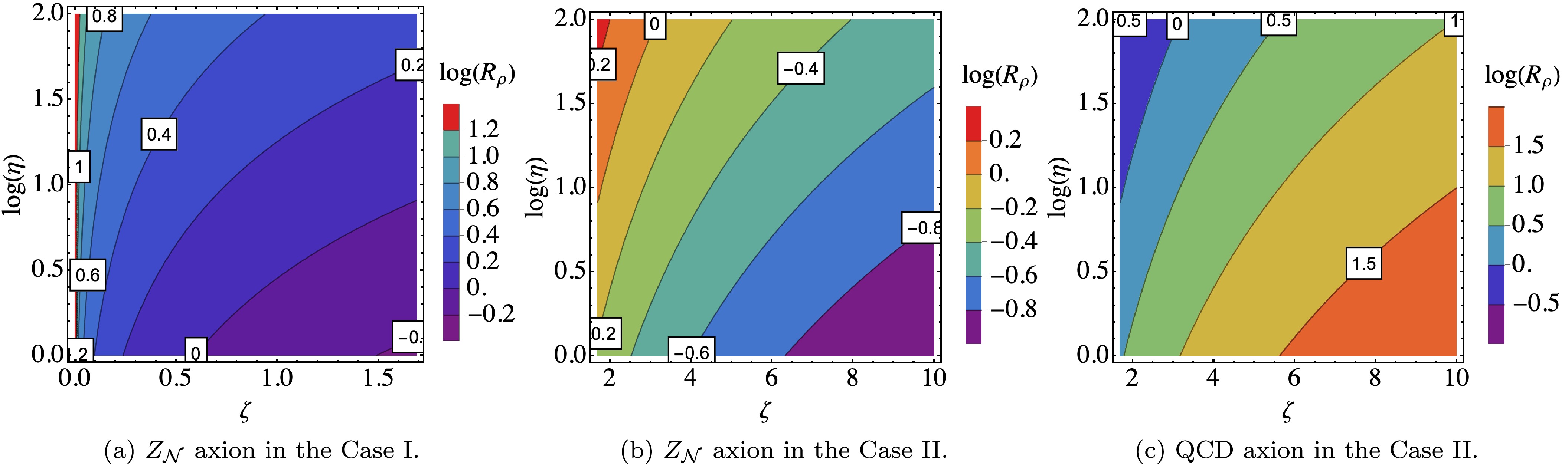

Figure 3.  (color online) Distributions of the axion relic density ratio $ \log(R_{\rho}) $ in the $ \{\zeta, \log(\eta)\} $ plane. The left, middle, and right panels represent the $ Z_{{\cal{N}}} $ axion in Case I, the $ Z_{{\cal{N}}} $ axion in Case II, and the QCD axion in Case II, respectively. Note that the initial misalignment angles are assumed to be of order one.

Next, we discuss the $ Z_{{\cal{N}}} $ axion DM in Case II. Because of the insights gained from the discussion in the last paragraph, we can simplify our discussion somewhat. We also begin with the QCD axion field, and its initial energy density at $ T_{1,a} $ is given by Eq. (23). Then, at $ T_\times<T<T_{1,a} $, the QCD axion energy density is adiabatic invariant, and at $ T_\times $ , it can be described by

At $ T=T_\times $, level crossing occurs, the light mass eigenvalue $ m_l(T) $ will comprise the $ Z_{{\cal{N}}} $ axion, and the energy density $ \rho_{a, \times} $ is transferred to the $ Z_{{\cal{N}}} $ axion $ \rho_{{{\cal{N}}},\times} $. To ensure this axion energy transition is adiabatic at $ T_\times $, we require the following condition to be satisfied:

where $ \Delta t_\times $ is the time interval corresponding to the temperature change described in Eq. (20). Additionally, we have verified this condition using the parameter set illustrated in the right panel of Fig. 1, and the results are presented in Fig. 4. Then, at $ T_{{\rm{QCD}}}<T<T_\times $, the adiabatic approximation is valid again, and the $ Z_{{\cal{N}}} $ axion energy density just before $ T_{{\rm{QCD}}} $ is given by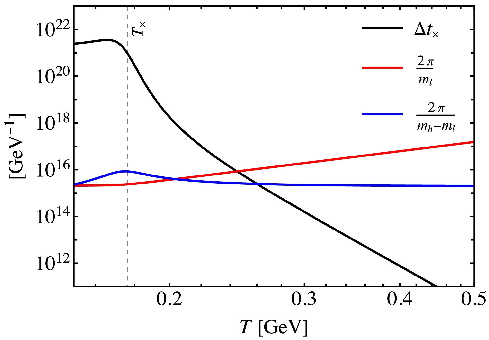

Figure 4.  (color online) The three terms in Eq. (31) as functions of temperature T. The black, red, and blue lines represent $ \Delta t_\times $, $ 2\pi/m_l(T) $, and $ 2\pi/(m_h(T)-m_l(T)) $, respectively. The gray dashed line represents $ T_\times\simeq 176.3\, {\rm{MeV}} $.

with mean velocity

The subsequent steps ($ T<T_{{\rm{QCD}}} $) are similar to those discussed in the previous paragraph. Substituting the mean velocity into Eq. (27), we have the present $ Z_{{\cal{N}}} $ axion energy density

Now, compared with the no mixing case, we find that the relic density can be modified by

As previously demonstrated, in the middle panel of Fig. 3, we present the distribution of $ R_{\rho} $ in the $ \{\zeta, \log(\eta)\} $ plane. In most regions, the ratio $ R_{\rho} $ can be suppressed, whereas in a small subset of regions, it can be enhanced. Note also that ζ is constrained by the set of $ {{\cal{N}}} $, and here, we only present a small range of zeta values, specifically $ 1.69<\zeta<10 $. Meanwhile, note that Eq. (35) resembles the single level crossing scenario, where the $ Z_{{\cal{N}}} $ axion mixes with ALP, leading to the suppression of the $ Z_{{\cal{N}}} $ axion relic density, as indicated by Eq. (25) of Ref. [22]. However, due to the differing ranges of parameters, here, ζ exceeds 1.69, and consequently, the $ Z_{{\cal{N}}} $ axion relic density ratio $ R_{\rho} $ can be either enhanced or suppressed.

Finally, we discuss the QCD axion DM in Case II. We should begin with the $ Z_{{\cal{N}}} $ axion field. It starts to oscillate at $ T_{1,{{\cal{N}}}} $ with the initial misalignment angle $ \theta_{1,{{\cal{N}}}} $, and the initial energy density is given by

At $ T_\times<T<T_{1,{{\cal{N}}}} $, the $ Z_{{\cal{N}}} $ axion energy density is adiabatic invariant, and at $ T_\times $, we have

At $ T=T_\times $, level crossing occurs, the heavy mass eigenvalue $ m_h(T) $ will comprise the QCD axion, and the energy density $ \rho_{{{\cal{N}}},\times} $ is transferred to the QCD axion $ \rho_{a,\times} $. Then, at $ T_0<T<T_\times $, the adiabatic approximation is valid again, and we have the present QCD axion energy density

Compared with the no mixing case, the relic density can be modified by

In the right panel of Fig. 3, we also present the distribution of $ R_{\rho} $ in the $ \{\zeta, \log(\eta)\} $ plane. We find that, within the parameter space we consider, the ratio $ R_{\rho} $ is enhanced in most regions, whereas it is suppressed in a minority of those regions. We also note that Eq. (39) resembles the level crossing that occurs in the mixing between the QCD axion and ALP, as illustrated by Eq. (3.26) of Ref. [29]. In such a case, the QCD axion relic density can be significantly suppressed. However, as mentioned earlier, due to the varying ranges of parameters, the QCD axion relic density ratio $ R_{\rho} $ in this context can be either enhanced or suppressed.

In summary, we have investigated the mass mixing between the canonical QCD axion and $ Z_{{\cal{N}}} $ axion and introduced a novel level crossing phenomenon. During the mixing, we find that level crossing can occur at the QCD phase transition critical temperature $ T_{{\rm{QCD}}} $ (Case I) or slightly before $ T_{{\rm{QCD}}} $ (Case II), depending on the ratio of the axion decay constants $ \zeta\sim 1.69 $. The conditions for level crossing to occur in Cases I and II are discussed in detail. In Case I, the zero-temperature QCD axion mass $ m_{a,0} $ should be smaller than the mass $ m_{{{\cal{N}}},\pi} $ and larger than the zero-temperature $ Z_{{\cal{N}}} $ axion mass $ m_{{{\cal{N}}},0} $, which can be characterized by the inequality $ 1.24\times 0.48^{{\cal{N}}/2} {{\cal{N}}}^{3/4}< \zeta<1.69 $. In Case II, the zero-temperature QCD axion mass $ m_{a,0} $ should be larger than $ m_{{{\cal{N}}},\pi} $ and the condition $ \zeta<{\cal{N}} $ should be satisfied, which can also be characterized by the inequality $ 1.69<\zeta<{{\cal{N}}} $. Note that, in this case, we also have a relatively weak constraint given by $ \zeta<1.69 \, \gamma^{-b} $, which becomes more stringent for large values of γ.

Despite the similarity in the cosmological evolution of mass eigenvalues in both cases, the transition of energy density between the axions differs. Specifically, in Case I, the axion energy transition at the level crossing is non-adiabatic (at $ T_{{\rm{QCD}}} $), while in Case II, it is considered to be adiabatic (at $ T_\times $). Finally, we estimate the relic density of the axion DM through the misalignment mechanism, focusing on the $ Z_{{\cal{N}}} $ axion DM in Cases I and II, as well as the QCD axion DM in Case II. We also compare this with other axion mixing scenarios and find that, within the parameter space we consider, the axion relic density can be either enhanced or suppressed. Furthermore, the level crossing phenomenon in this scenario may have other intriguing cosmological implications, such as gravitational waves and primordial black holes.

The appendix is organized as follows. In App. A, we provide an illustrative example of the UV completion for the$Z_{{\cal{N}}} $ axion. In App. B, we present the temperature-dependent mass of the $Z_{{\cal{N}}} $ axion. In App. C, we describe how our axion mixing potential is derived. Finally, in App. D, we present some details about the axion relic density, considering both the no-mixing and mixing scenarios.

Here, we provide an illustrative example of the UV completion for the $ Z_{{\cal{N}}} $ axion. We consider the KSVZ $ Z_{{\cal{N}}} $ axion scenario [16], with $ {{\cal{N}}} $ copies of vector-like Dirac fermions $ Q_k $ and a gauge singlet complex scalar S. The $ Z_{{\cal{N}}} $ symmetry reads $ Q_k\to Q_{k+1} $, $S\to {\rm e}^{2\pi {\rm i}/{{\cal{N}}}}S$. The general Lagrangian is given by

which exhibits an accidental U(1)$ _{{\rm{PQ}}} $ symmetry that is spontaneously broken by the vacuum expectation value $ v_S $ through the potential $ V(S, H_k) $. The complex scalar S can be expressed as

where ρ and φ represent the radial and angular (axion) modes, respectively. Through an axial transformation, the axion mode can be rotated away from the Yukawa term. After integrating out the heavy quarks, the resulting effective Lagrangian for the axion is given by

where we set $ v_S=F_a $, $ F_a $ is the axion decay constant, $ \alpha_s $ is the strong fine structure constant, and $ G_k $ and $ \widetilde{G}_k $ are the gluon field strength tensor and dual tensor, respectively.

In the context of the KSVZ $ Z_{{\cal{N}}} $ axion model, the discrete symmetry is inherently present due to its construction. By elevating the inherent $ Z_{{\cal{N}}} $ symmetry to a gauge symmetry, an accidental U(1)$ _{{\rm{PQ}}} $ invariance arises, which, for large values of $ {{\cal{N}}} $, is efficiently shielded from additional sources of explicit breaking. Furthermore, the lowest-dimensional PQ-violating operator in the scalar potential that is compatible with the $ Z_{{\cal{N}}} $ symmetry is $ S^{{\cal{N}}} $, which contributes an explicitly PQ-breaking term to the potential.

See also Ref. [16] for another UV completion involving the composite $ Z_{{\cal{N}}} $ axion model.

Here, we provide a brief overview of the temperature-dependent $ Z_{{\cal{N}}} $ axion mass. As derived in Ref. [16], the zero-temperature ($ T\leq T_{{\rm{QCD}}} $) $ Z_{{\cal{N}}} $ axion potential is given by

with the zero-temperature axion mass

where $ z\equiv m_u/m_d\simeq 0.48 $. At medium temperatures $ T_{{\rm{QCD}}}<T\leq T_{{\rm{QCD}}}/\gamma $, the $ Z_{{\cal{N}}} $ axion potential is given by

where $ V(\theta) $ is the QCD axion zero-temperature chiral potential

Using

we obtain the axion mass

which is also defined as the mass $ m_{{{\cal{N}}},\pi} $. At high temperatures $ T>T_{{\rm{QCD}}}/\gamma $, the $ Z_{{\cal{N}}} $ axion potential is given by

Then, we have the axion mass

Note that the temperature parameter γ delineates the high-temperature and intermediate-temperature regions. To be more precise, this parameter can be represented by the inequality $ \gamma_{{\rm{min}}} < \gamma < \gamma_{{\rm{max}}} $, where the values of γ at the lower and upper bounds correspond to the mirror copies of the SM that are the coldest and hottest, respectively. For simplicity, we denote it as γ. Finally, the temperature-dependent $ Z_{{\cal{N}}} $ axion mass can be described by

See also Ref. [17] for more details.

In this section, we describe how our axion mixing potential, which is presented in Eq. (1), is derived. Let us first consider the mixing of two axions $ \phi_1 $ and $ \phi_2 $ with the mixing potential

where $ n_{ij} $ are the domain wall numbers, and $ \delta_{i} $ are the constant phases. To discuss the emergence of the level crossing phenomenon, the domain wall numbers must be set in the following manner:

or

In other words, among these domain wall numbers, one must be set to zero, while the rest cannot be zero. This consideration and operation are reasonable, and numerous pieces of literature considering the mixing between two axions have adopted similar approaches, e.g., the mixing between the QCD axion and ALP [20] or sterile axion [21], as well as the mixing between the $ Z_{{\cal{N}}} $ axion and ALP [22]. Note that Refs. [20] and [21] can be viewed as corresponding to the considerations in the contexts of Eqs. (C2) and (C3), respectively, if we consider $ \phi_1 $ as the QCD axion and $ \phi_2 $ as the ALP. In these contexts, the domain wall numbers are equal to or less than 1 (and there is exactly one that is less than 1, $ i.e. $, 0). In contrast, in Ref. [22] the domain wall numbers can be greater than 1. However, the constant phases must be set to zero:

This can be regarded as tantamount to demanding an independent solution for addressing the strong CP problem. Because this assumption has no impact on the evolution of the two axion fields during the mixing process, it will not alter the energy density of axions in the context of mass mixing [29].

Now, consider the scenario of multiple QCD axions mixing in this work, specifically one QCD axion ϕ and one $ Z_{{\cal{N}}} $ axion φ. For our purposes, we must consider the following parameter settings:

Therefore, we obtain the mixing potential in Eq. (1), which is given by

As mentioned above, obtaining the axion mixing potential here is both straightforward and reasonable. When we set $ n_{11}=1 $ and $ n_{12}=0 $, the first term of Eq. (C6) aligns perfectly with the canonical QCD axion potential; however, this alignment is not an absolute requirement in this context. Additionally, it is worth noting that the acquisition of the mixing potential here differs from the acquisition of the single $ Z_{{\cal{N}}} $ axion potential. Furthermore, there should exist another mixing scenario with the potential given by

The corresponding cosmological implications would be entirely distinct and warrant a separate detailed discussion; however, such discussions are beyond the scope of this particular context.

In this section, we present some details about the axion relic density through the misalignment mechanism. We consider the pre-inflationary scenario, in which the PQ symmetry is spontaneously broken during inflation.

We first show the QCD axion relic density without mixing. At high temperatures $ T\gg T_{{\rm{QCD}}} $, the QCD axion field is frozen at an arbitrary initial misalignment angle $ \theta_{1,a} $ and starts to oscillate at $ T_{1,a} $. The oscillation temperature $ T_{1,a} $ is given by

with the Hubble parameter

with the number of effective degrees of freedom of energy density $ g_* $ and reduced Planck mass $ M_{{\rm{Pl}}}\simeq 2.4\times 80^{18}\; {\rm{GeV}} $. The initial energy density in the QCD axion field is

where $ m_{a,1} $ is the axion mass at $ T_{1,a} $. At $ T_0<T<T_{1,a} $, the QCD axion energy density is adiabatic invariant with the comoving number $ N_a \equiv \rho_a a^3 /m_a $, where a is the scale factor. Using

the present QCD axion energy density ($ T_0 $) can be described by

where $ a_{1,a} $ and $ a_0 $ are the scale factors at $ T_{1,a} $ and $ T_0 $, respectively.

Next, we show the $ Z_{{\cal{N}}} $ axion relic density without mixing. At high temperatures $ T> T_{{\rm{QCD}}} $, the $ Z_{{\cal{N}}} $ axion field is frozen at an initial misalignment angle $ \theta_{1,{{\cal{N}}}} $ and starts to oscillate at the oscillation temperature $ T_{1,{{\cal{N}}}} $. Here, we consider a case that the $ Z_{{\cal{N}}} $ axion mass is temperature-dependent at the first oscillation, $ i.e. $, $ T_{1,{{\cal{N}}}}> 1/\gamma T_{{\rm{QCD}}} $. The initial energy density in the $ Z_{{\cal{N}}} $ axion field is

where $ m_{{{\cal{N}}},1} $ is the axion mass at $ T_{1,{{\cal{N}}}} $. At $ T_{{\rm{QCD}}}<T<T_{1,{{\cal{N}}}} $, the $ Z_{{\cal{N}}} $ axion energy density is adiabatic invariant with the comoving number $ N_{{\cal{N}}} \equiv \rho_{{\cal{N}}} a^3 /m_{{\cal{N}}} $. Then, we have the $ Z_{{\cal{N}}} $ axion energy density at $ T_{{\rm{QCD}}} $ as

where $ a_{{{\cal{N}}},a} $ is the scale factor at $ T_{1,{{\cal{N}}}} $. In this period, the $ Z_{{\cal{N}}} $ axion is trapped around $ \theta_{{\rm{tr}}}\equiv\theta_{{\cal{N}}}(T_{{\rm{QCD}}})\sim \pi $ until the QCD phase transition with the initial axion velocity $ \dot{\theta}_{{\rm{tr}}}\equiv\dot{\theta}_{{\cal{N}}}(T_{{\rm{QCD}}}) $ occurs. Then, the mean velocity is given by

At $ T=T_{{\rm{QCD}}} $, the $ Z_{{\cal{N}}} $ axion mass is exponentially suppressed due to the $ Z_{{\cal{N}}} $ symmetry, and the true minimum develops. Note that the axion energy density at $ T_{{\rm{QCD}}} $ is non-adiabatic, which can then be described by

The follow-up is determined by the velocity $ \dot{\theta}_{{\rm{tr}}}\sim 2m_{{\cal{N}}}/{{\cal{N}}} $, and we consider a case that the axion has a large initial velocity, $ i.e. $, $ \dot{\theta}_{{\rm{tr}}}\gg 2m_{{\cal{N}}}/{{\cal{N}}} $. Then, at $ T_2<T<T_{{\rm{QCD}}} $, the $ Z_{{\cal{N}}} $ axion energy density is conserved with the PQ charge $ q_{{\rm{kin}}}=\dot{\theta}_{{\cal{N}}} a^3 $, and here, $ T_2 $ is defined as the temperature at which the kinetic energy is comparable to the barrier height, $ \dot{\theta}_{{\cal{N}}}(T_2)=2m_{{\cal{N}}}/{{\cal{N}}} $. Using the conserved $ q_{{\rm{kin}}} $, the scale factor at $ T_2 $ is given by

At $ T<T_2 $, the $ Z_{{\cal{N}}} $ axion will start to oscillate until the present, and the axion energy density is adiabatic invariant. Then, using

the $ Z_{{\cal{N}}} $ axion energy density at present can be described by

Substituting the mean velocity, we obtain the axion energy density

where $ C\simeq 2 $ is a constant.

The axion relic density ratio $ R_{\rho} $ in this case is given by

The axion relic density ratio $ R_{\rho} $ in this case is given by

The axion relic density ratio $ R_{\rho} $ in this case is given by