


 Abstract
 HTML
HTML Reference
 Related
 PDF
PDF


-
Weak decays of heavy mesons not only provide a unique platform to test the electroweak structures of the Standard Model (SM), but can also shed light on new physics (NP) beyond the SM. Among different species of heavy mesons, the
$ B^+_c $ ① meson, discovered in 1998 by the CDF collaboration [1, 2], is of particular interest in this regard. The$ B^+_c $ meson has specific production and decay mechanisms, and accordingly the measurement of its mass, lifetime and decay branching ratios would help to probe the underlining quark dynamics and determine SM parameters.Consisting of two heavy quarks of different types, the
$ B^+_c $ meson has three decay categories: 1) b-quark decay with spectator c-quark; 2) c-quark decay with spectator b-quark; 3) annihilation processes (e.g.$ B^+_c \to \tau^+\nu_\tau, c\overline{s} $ ). The purely leptonic decay through the annihilation process is sensitive to the decay constant$ f_{B_c} $ and the CKM matrix element$ |V_{cb}| $ . Such a scheme has been used for the determination of$ |V_{cd}| $ and$ |V_{cs}| $ in$ D^+/D^+_s \to \tau^+\nu_\tau, \mu^+\nu_\mu $ [3]. For$ |V_{cb}| $ , since the$ B^+_c \to \tau^+\nu_\tau $ channel has not been discovered, it is measured using inclusive semileptonic$ b \to c $ transitions and the exclusive channel of$ \overline{B} \to D^*l\overline{\nu}_l $ . However, even if$ B^+_c \to \tau^+\nu_\tau $ had been discovered, the decay$ \overline{B} \to D^*l\overline{\nu}_l $ would still provide a more precise$ |V_{cb}| $ measurement.In recent years a few discrepancies have been found between the SM predictions and different experimental measurements in the bottom sector, especially in tauonic decay modes of B mesons [4-6]. In view of there being no clear signal in the direct searches for NP to date, the implications in low-energy processes are of great importance. Studies of tauonic decay modes of B mesons, mostly
$ B\to D(^*)\tau\nu $ decays, have given some hints of lepton flavor universality violation. While these decay modes are very sensitive to vector/axial-vector type interactions, the (pseudo)scalar type interactions which can be induced in many popular NP models, e.g. the two-Higgs-doublet and leptoquark models, are less constrained by them. Due to the mass hierarchy$ m_\tau\ll m_{B_c} $ that results in helicity suppression for$ B^+_c \to \tau^+\nu_\tau $ with$ V-A $ interactions in the SM,$ B_c\to\tau\nu $ has a better sensitivity to the (pseudo)scalar NP interactions [7, 8]. Therefore, measurement of the branching ratio$ {\cal B}(B^+_c \to \tau^+\nu_\tau) $ can be a key in the search for NP. As we will show in Sec. II, based on the current state of knowledge, NP can affect$ {\cal B}(B^+_c \to \tau^+\nu_\tau) $ significantly, which highlights the importance of studying this quantity in the future.The recently proposed CEPC (Circular Electron Positron Collider) [9] provides an excellent opportunity to measure
$ {\cal B}(B^+_c \to \tau^+\nu_\tau) $ . It is planned to have a circumference of 100 km and two interaction points. Its primary objective is precision Higgs studies at a center-of-mass-energy$ (\sqrt{s} $ ) of 240 GeV, with a nominal production of$ 10^6 $ Higgs bosons. In addition, a dedicated$ WW $ threshold scan$(\sqrt{s} = 158-172 $ GeV) and the Z factory mode$ (\sqrt{s} = 91.2 $ GeV) will be operated for electroweak and flavor physics studies. The Z factory will produce up to one trillion Z bosons (Tera-Z) in two years, far exceeding LEP's production [10]. Such a huge data sample will enable high precision tests of the SM and allow the study of many previously unobservable processes. Furthermore, the clean$ e^+e^- $ collision environment and the well-defined initial state compared to hadron colliders are advantages for this analysis at the CEPC. (Super) B factories operating at the$ \Upsilon $ (4S) center-of-mass-energy are below the energy threshold for$ B^+_c $ production. A detailed discussion of the various advantages and prospects of flavor studies at the CEPC can be found in Ref. [9].In this paper, we discuss the potential of measuring the processes
$ B^+_c \to \tau^+\nu_\tau $ ,$ \tau^+ \to e^+\nu_e\overline{\nu}_\tau $ and$ \tau^+ \to \mu^+\nu_\mu\overline{\nu}_\tau $ in$ Z \to b\overline{b} $ at the CEPC. Important backgrounds are other$ Z \to c\overline{c} $ and$ Z \to b\overline{b} $ processes, especially the decay of$ B^+ \to \tau^+\nu_\tau $ in$ Z \to b\overline{b} $ events②. Both$ B^+_c $ and$ B^+ $ have similar masses and event topologies [3]. The main difference is the lifetime (the$ B^+_c $ lifetime is around one third of the$ B^+ $ lifetime). The L3 experiment at LEP searched for$ B^+ \to \tau^+\nu_\tau $ in 1997 with$ 1.475 \times 10^6 $ $ Z \to q\overline{q} $ events [11], and determined$ {\cal B}(B^+ \to \tau^+\nu_\tau) < 5.7 \times 10^{-4} $ at 90% CL. That study did not consider the contribution from$ B^+_c \to \tau^+\nu_\tau $ . However, Refs. [12, 13] later argued that the$ B^+_c \to \tau^+\nu_\tau $ contribution could be comparable to the$ B^+ \to \tau^+\nu_\tau $ contribution, and that a similar analysis method could be used to measure$ B^+_c \to \tau^+\nu_\tau $ . Understanding the$ B^+ \to \tau^+\nu_\tau $ background is crucial in this analysis.We estimate the
$ B^+_c/B^+ \to \tau^+\nu_\tau $ event yield at the CEPC Z pole as follows. The number of$ B^+ \to \tau^+\nu_\tau $ events produced is given by:$ \begin{split} N(B^\pm \to \tau^\pm\nu_\tau) = & N_Z \times {\cal B}(Z \to b\overline{b}) \times 2 \times f(\overline{b} \to B^+ X) \\ & \times {\cal B}(B^+ \to \tau^+\nu_\tau) \,, \end{split} $

(1) where
$ N_Z $ is the total number of Z bosons produced. The factor two accounts for the quark anti-quark pair. The branching ratios$ {\cal B}(Z \to b\overline{b}) = 0.1512 \pm 0.0005 $ ,$ f(\overline{b} \to B^+ X) = 0.408 \pm 0.007 $ , and$ {\cal B}(B^+ \to \tau^+\nu_\tau) = (1.09 \pm 0.24) \times 10^{-4} $ are taken from Ref. [3]. For the$ B_c $ production, the theoretical result at next-to-leading order in$ \alpha_s $ gives$ {\cal B}(Z\to B^\pm_cX) = 7.9\times 10^{-5} $ [14], and our estimate of$ {\cal B}(B^+_c \to \tau^+\nu_\tau) $ (see the next section) is$ (2.36 \pm 0.19) $ %. These numbers give$ R_{B_c/B} = \frac{N(B^\pm_c \to \tau^\pm\nu_\tau)}{N(B^\pm \to \tau^\pm\nu_\tau)} = 0.28 \pm 0.05, $

(2) where we use
$ R_{B_c/B} $ to denote the ratio. Note that the actual uncertainty for$ R_{B_c/B} $ is larger since we lack the uncertainty for$ {\cal B}(Z\to B^\pm_cX) $ . We conduct our analysis with$ 10^{9} $ simulated Z boson decays including$ (1.3 \pm 0.3) \times 10^4 $ $ B^\pm \to \tau^\pm\nu_\tau $ events. For simplicity and to give a larger signal dataset for analysis, we assume both$ N(B^\pm_c/B^\pm \to \tau\nu_\tau) $ are equal to$ 1.3 \times 10^4 $ and discuss other scenarios at the end, since the results are easily scalable for different values of$ R_{B_c/B} $ .The rest of this paper is organized as follows. Section II gives the decay width of
$ B^+_c \to \tau^+\nu_\tau $ in the SM and estimates the effects in NP scenarios. Section III introduces the detector, software and the MC-simulated event samples. Section IV presents the analysis method and results. The conclusion is given in Sec. V. -
In the SM, the decay width of the purely leptonic decay
$ B^+_c \to l^+\nu_l $ is given by:$ \varGamma_{ \rm{SM}} (B^+_c \to l^+\nu_l) = \frac{G^2_F}{8\pi}|V_{cb}|^2 f^2_{B_c} m_{B_c} m^2_l \left(1 - \frac{m^2_l}{m^2_{B_c}}\right)^2 \,, $

(3) where
$ G_F $ is the Fermi coupling constant,$ V_{cb} $ is the CKM matrix element,$ f_{B_c} $ is the decay constant, and$ m_{B_c} $ ,$ m_l $ are the masses of the meson and the charged lepton, respectively. Due to helicity suppression, the$ \tau $ final state has the largest branching fraction. The measurement of$ B^+_c \to \tau^+\nu_\tau $ would help to determine the fundamental parameter$ |V_{cb}| $ , once the decay constant is known from first-principle calculations, i.e. lattice QCD. The Feynman diagram for$ B^+_c \to \tau^+\nu_\tau $ in the SM is shown in the left-hand panel of Fig. 1.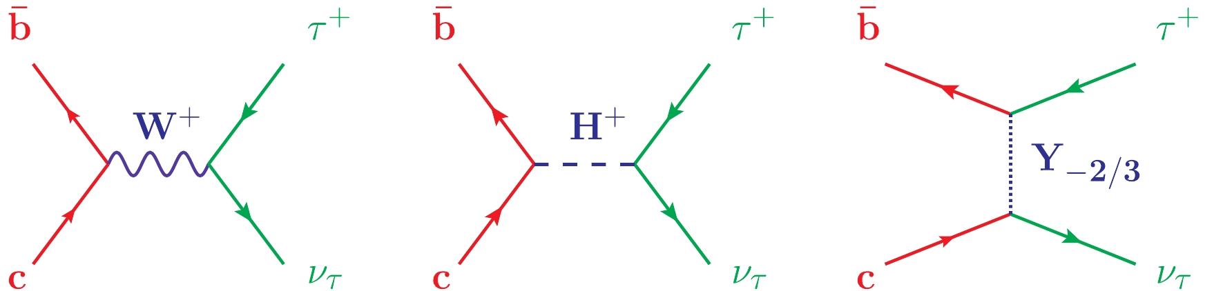
Figure 1. (color online) Feynman diagrams for tauonic
$ B_c $ decays in the SM, 2HDM and LQ models.With the decay constant
$ f_{B_c} = (0.434\pm0.015)\; {\rm{GeV}} $ [15],$ \tau(B_c) = (0.510\pm 0.009)\times 10^{-12}\; \rm{s} $ and$ |V_{cb}| = (42.2 \pm 0.8) \times 10^{-3} $ [3], we obtain$ {\cal B}(B^+_c \to \tau^+\nu_\tau) = (2.36\pm0.19){\text{%}} \,, $

(4) where the errors from the decay constant and lifetime of the
$ B^+_c $ have been added in quadrature. The uncertainty in the$ B^+_c $ branching fraction is dominated by the decay constant, which might be further reduced in a more accurate lattice QCD calculation in the future. Other theoretical studies on the subject of$ B^+_c $ decay can be found in Ref. [16].Since the tau lepton has the largest mass compared to the other two species of lepton, the NP coupling might have a more evident effect in tauonic decays of heavy mesons. Two popular types of NP model are the two-Higgs-doublet model (2HDM) with a charged Higgs boson propagator similar to the W boson propagator, and the leptoquark (LQ) models that couple leptons with quarks. The charged Higgs boson in 2HDM can have a significant coupling with the tau, and thereby its contributions to decay widths could be sizable [17, 18].
Theoretical studies of NP contributions can be conducted in two distinct ways. One is to confront the explicit model predictions one by one with available experimental constraints, while the other is to employ an effective field theory (EFT) approach. Integrating out the massive particles, e.g. charged Higgs particle or the LQ in Fig. 1, the NP contributions are incorporated into a few effective operators, with the interaction strengths embedded in Wilson coefficients. A general effective Hamiltonian for the
$ b\to c\tau\nu $ transition can be written as$ \begin{aligned}[b] {\cal{H}}_{\rm{eff}} =&\frac{4 G_{F}}{\sqrt{2}} V_{c b}\left[\left(1+C_{V_{1}}\right) {O}_{V_{1}}+C_{V_{2}} {O}_{V_{2}} \right. \\ &\left.+C_{S_{1}} {O}_{S_{1}}+C_{S_{2}} {O}_{S_{2}}\right]+{\rm{h}}.{\rm{c}}. \,, \end{aligned} $

(5) where
$ {O}_i $ are four-fermion operators and$ C_i $ are the corresponding Wilson coefficients. The four-fermion operators are defined as$ \begin{aligned}[b] {O}_{V_{1}} =& \left(\bar{c}_{L} \gamma^{\mu} b_{L}\right)\left(\bar{\tau}_{L} \gamma_{\mu} \nu_{L}\right), \\ {O}_{V_{2}} =& \left(\bar{c}_{R} \gamma^{\mu} b_{R}\right)\left(\bar{\tau}_{L} \gamma_{\mu} \nu_{L}\right), \\ {O}_{S_{1}} =& \left(\bar{c}_{L} b_{R}\right)\left(\bar{\tau}_{R} \nu_{L}\right), \\ {O}_{S_{2}} =& \left(\bar{c}_{R} b_{L}\right)\left(\bar{\tau}_{R} \nu_{L}\right), \end{aligned} $

(6) where
$ {O}_{V_{1}} $ is the only operator present in the SM. The 2HDM can contribute to$ {O}_{S_{1}} $ , while the LQs can have more versatile contributions depending on their spin and chirality in couplings.Having Eq. (5) and Eq. (6) at hand, one arrives at
$ \frac{\varGamma_{ \rm{eff}}(B^+_c \to \tau^+\nu_\tau)}{\varGamma_{ \rm{SM}}(B^+_c \to \tau^+\nu_\tau)} = \left| 1+C_{V_1}-C_{V_2}+C_{S_1}\frac{m_{B_c}^0}{m_\ell}-C_{S_2}\frac{m_{B_c}^0}{m_\ell} \right|^2 \,, $

(7) where
$ m_{B_c}^0\equiv m_{B_c}^2/(m_b+m_c) $ . This expression shows the deviation of decay width of$ B^+_c \to \tau^+\nu_\tau $ compared with the SM.Inspired by the experimental measurements of
$ B\to D(^*)\tau\nu $ and other decays induced by$ b\to c \tau\nu $ , quite a few theoretical analyses of NP contributions have been made in recent years. In this work, we will make use of the results for the Wilson coefficients from Refs. [19, 20]:$ |1+ {\rm{Re}}[C_{V_1}]|^2 +|{\rm{Im}} [C_{V_1}]|^2 = 1.189\pm0.037 \,, $

(8) $ C_{V_2} = (-0.022\pm 0.033) \pm (0.414\pm 0.056) {\rm i} \,, $

(9) $ C_{S_1} = (0.206\pm 0.051) + (0.000\pm 0.499){\rm i} \,, $

(10) $ C_{S_2} = (-1.085\pm 0.264) \pm (0.852\pm 0.132){\rm i}, $

(11) and the masses:
$ \begin{array}{c} m_{B_c} = 6.2749 \; {\rm{GeV}}\,, \qquad m_b = 4.18 \; {\rm{GeV}}\,, \\ m_c = 1.27 \; {\rm{GeV}}\,, \qquad m_\tau = 1.77686 \; {\rm{GeV}}. \end{array} $

(12) Equation (8) directly implies that the branching fraction of
$ B^+_c \to \tau^+\nu_\tau $ can be affected by$ (18.9\pm3.7)$ % if only the SM-like$ V-A $ operator$ {O}_{V_1} $ is included. If$ {O}_{V_2} $ is considered, the contributions to$ (\varGamma_{ \rm{eff}} - \varGamma_{ \rm{SM}})/\varGamma_{ \rm{SM}} $ are shown in Fig. 2. The red shaded areas in this figure correspond to the global fitted results of data on B meson decays induced by$ b\to c\tau\nu $ , as shown in Eq. (9). In this figure and the following ones, we do not consider the correlation between the real and imaginary part in the Wilson coefficients. Two branches are found due to the ambiguous sign in the imaginary part of$ C_{V_2} $ . From this figure, one can infer that the NP contributions range from about 10% to 30%. In these two scenarios, branching fractions of$ B^+_c \to \tau^+\nu_\tau $ are mildly affected due to helicity suppression.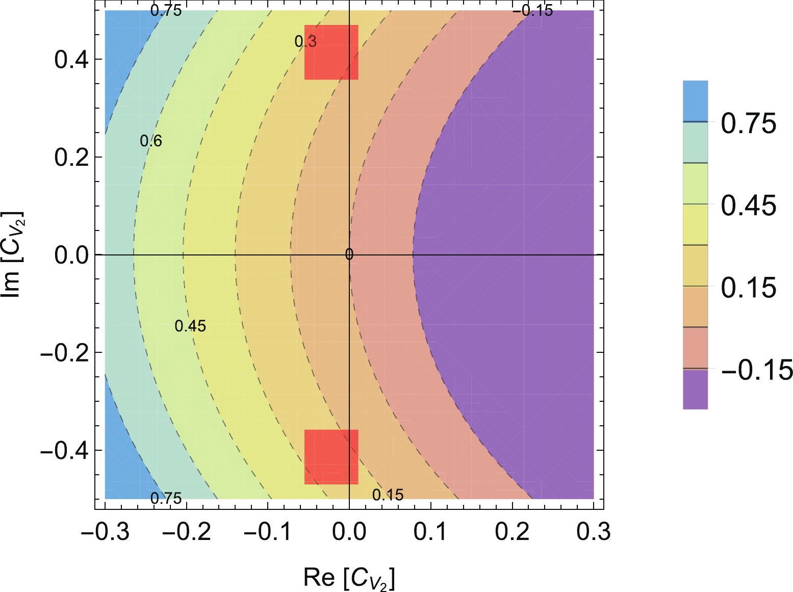
Figure 2. (color online) Sensitivities of
$ (\varGamma_{ \rm{eff}} - \varGamma_{ \rm{SM}})/\varGamma_{ \rm{SM}} $ (100%) to$ C_{V_2} $ . The SM lies at the origin with$ {\rm{Re}}[C_{V_2}] = {\rm{Im}}[C_{V_2}] = 0 $ . Labels (in units of 100%) on contours denote the modification of branching ratios (decay widths) with respect to the SM values. The red shaded areas correspond to the global fitted results of available data on$ b\to c\tau\nu $ decays, as shown in Eq. (9). These areas deviate from the SM predictions by about a few$ \sigma $ .If we switch to
$ {O}_{S_1} $ , the results are shown in Fig. 3, and again the red shaded area corresponds to the global fitted results shown in Eq. (10). Similar results are shown in Fig. 4 for$ {O}_{S_2} $ . In these two figures, one can clearly see that$ \varGamma(B^+_c \to \tau^+\nu_\tau) $ is dramatically affected by NP contributions. At this stage the errors do not allow a very conclusive result on the existence of NP, and accordingly measurements of this width at CEPC would help to confirm or rule out these NP scenarios.
Figure 3. (color online) Sensitivities of
$ (\varGamma_{ \rm{eff}} - \varGamma_{ \rm{SM}})/\varGamma_{ \rm{SM}}$ (100%) to$ C_{S_1} $ . The SM lies at the origin with$ {\rm{Re}}[C_{S_1}] = {\rm{Im}}[C_{S_1}] = 0 $ . Labels (in units of 100%) on contours denote the modification of branching ratios (decay widths) with respect to the SM values. The red shaded area corresponds to the global fitted results of available data on$ b\to c\tau\nu $ decays, as shown in Eq. (10).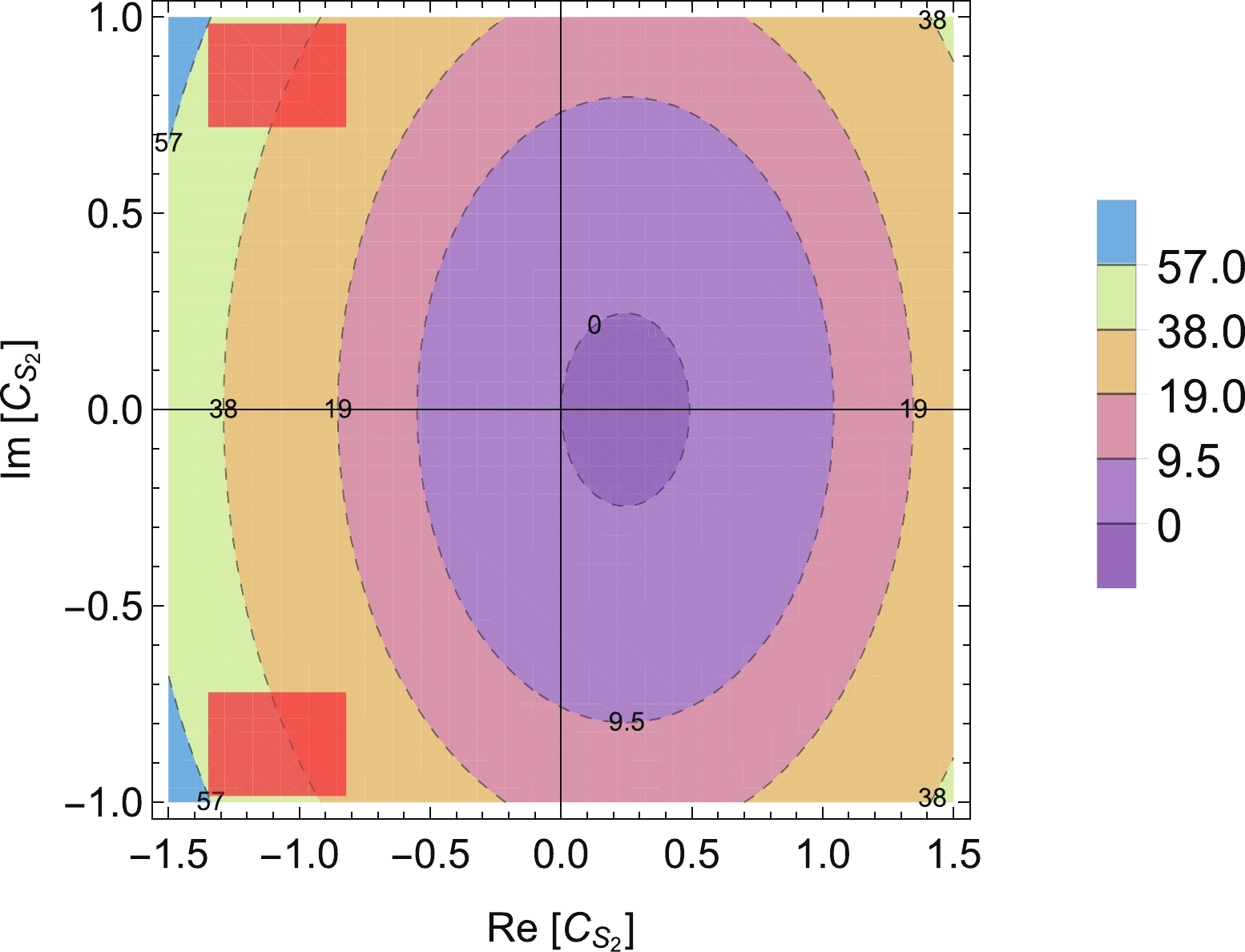
Figure 4. (color online) Similar to Fig. 3, with red shaded areas as parameter spaces of
$ C_{S_2} $ given in Eq. (11).Next, let us consider the
$ |V_{cb}| $ measurement in the SM scenario. Its uncertainty can be derived from the relative uncertainty of the signal strength$ \sigma (\mu)/\mu $ . The signal strength$ \mu $ is the ratio between the measured effective cross section and the corresponding SM prediction, and$ \sigma(\mu) $ is its uncertainty. Therefore it is straightforward that:$ \begin{aligned}[b] \frac{\sigma (\mu)}{\mu} =& \frac{\sigma(N(B^\pm_c \to \tau\nu_\tau))}{N(B^\pm_c \to \tau\nu_\tau)} \\=& \frac{\sigma({\cal B}(Z \to B^\pm_cX) {\cal B}(B^+_c \to \tau^+\nu_\tau))}{{\cal B}(Z \to B^\pm_cX) {\cal B}(B^+_c \to \tau^+\nu_\tau)}\\ =& \frac{\sigma({\cal B}(Z \to B^\pm_c) \varGamma_{ \rm{SM}}(B^+_c \to \tau^+\nu_\tau)/\varGamma(B^+_c))}{{\cal B}(Z \to B^\pm_c) \varGamma_{ \rm{SM}}(B^+_c \to \tau^+\nu_\tau)/\varGamma(B^+_c)}, \end{aligned} $

(13) where
$ \varGamma(B^+_c) $ is the total width of the$ B^+_c $ . Substituting Eq. (3) into the above equation, we have:$ \begin{aligned}[b] \left( \frac{\sigma(\mu)}{\mu} \right )^2 =& \left ( \frac{\sigma({\cal B}(Z \to B^\pm_c X))}{{\cal B}(Z \to B^\pm_c X)} \right )^2 + 4\left ( \frac{\sigma(|V_{cb}|)}{|V_{cb}|} \right )^2 \\&+ 4\left ( \frac{\sigma(f_{B_c})}{f_{B_c}} \right )^2 + \left ( \frac{\sigma(\varGamma(B^+_c))}{\varGamma(B^+_c)} \right )^2\\& + \rm{Cov.} +{\cal{O}}(10^{-6}), \end{aligned} $

(14) where Cov. refers to the covariances between variables. The
$ \sigma(f_{B_c})/f_{B_c} $ and$ \sigma(\varGamma(B^+_c))/\varGamma(B^+_c) $ are both at$ {\cal{O}} $ (1%) level. Section IV shows that$ \sigma(\mu)/\mu $ is also likely at 1% level at Tera-Z. This leaves the error terms to be dominated by the$ B^+_c $ production term, which has a much bigger uncertainty, and will determine the uncertainty of$ |V_{cb}| $ . If the$ B^+_c $ production term can be determined to$ {\cal{O}} $ (1%) level in the future and the covariances are also around the same level or less,$ |V_{cb}| $ could be determined to$ {\cal{O}} $ (1%) level as well. -
The CEPC CDR (Conceptual Design Report) [9] provides a detailed description of the detector setup and the software infrastructure. These are both inspired by the International Large Detector (ILD) of the International Linear Collider (ILC) and offer comparable performances. The general flow of software is as follows: 1) create simulated event samples using Pythia [21] and Whizard [22]; 2) MokkaPlus [23], a GEANT4 [24] based simulation tool, simulates the interaction with the detector; 3) the reconstruction framework mimics the electronics responses and employs Arbor [25] and LICH [26] for physics object creation and lepton identification. Upon completing the standard procedures, two more software packages are used for further analysis. One is LCFIPlus [27], an ILC software package which can perform jet clustering and flavor tagging operations to separate different quark flavors in
$ Z \to q\overline{q} $ . The other is TMVA [28], a multi-variable analysis tool for BDT (boosted decision tree) training.The simulated sample consists of
$ Z \to q\overline{q}, B^+ \to \tau^+\nu_\tau $ and$ B^+_c \to \tau^+\nu_\tau $ . The latter two are additional$ Z \to q\overline{q} $ events that contain the corresponding processes. In order to save time, only a fraction of the$ q\overline{q} $ (not including$ B^+_c/B^+ \to \tau^+\nu_\tau $ ) events that are sufficient for analysis are actually simulated. The data are then scaled to reach the sample size corresponding to$ 10^9 $ Z boson decays. For the$ B^+_c/B^+ \to \tau^+\nu_\tau $ , we simulated one million events each, and the final numbers and histograms are correspondingly scaled down. All of the scaling factors are shown in Table 1 and Table 2.$B^\pm_c \to \tau\nu_\tau$ (0.013)

$B^\pm \to \tau\nu_\tau$ (0.013)

$d\overline{d}(15)$ +

$u\overline{u}(12)$ +

$s\overline{s}(15)$ 

$c\overline{c} (4.8)$ 

$b\overline{b}(3.25)$ 

$\tau \to e\nu\overline{\nu}$ 

excl. $\tau \to e\nu\overline{\nu}$ 

$\tau \to e\nu\overline{\nu}$ 

excl. $\tau \to e\nu\overline{\nu}$ 

All events 2,303 10,691 2,270 10,633 419,928,342 119,954,033 151,286,603 b-tag > 0.6 1,611 7,463 1,547 7,151 2,134,617 7,344,014 116,723,067 Energy asymmetry > 10 GeV 1,425 6,184 1,389 5,801 486,762 1,609,771 30,064,030 Has electron in signal hemisphere 1,273 1,300 1,243 1,132 143,595 625,670 15,905,613 Electron is the most energetic particle 915 116 859 93 8,490 79,190 4,587,248 $E_B > 20$ GeV

909 112 852 88 981 34,147 3,203,073 $1^{\rm{st}}$ BDT score > 0.99

390 12 259 4 — 48 910 $2^{\rm{nd}}$ BDT score > 0.4

199 $12^\star$ 

73 $4^\star$ 

— $48^\star$ 

33 Table 1. The cut chain for the electron final state for
$ 10^9 $ Z bosons. The numbers in parentheses are corresponding scale factors. In the final row, the numbers with stars mean the corresponding channels are not used in the second BDT training in order to avoid possible overfitting. Instead, we make a conservative assumption that all of the events which pass the first BDT cut survive the second BDT cut.$B^\pm_c \to \tau\nu_\tau$ (0.013)

$B^\pm \to \tau\nu_\tau$ (0.013)

$d\overline{d}(15)$ +

$u\overline{u}(12)$ +

$s\overline{s}(15)$ 

$c\overline{c} (4.8)$ 

$b\overline{b}(3.25)$ 

$\tau \to \mu\nu\overline{\nu}$ 

excl. $\tau \to \mu\nu\overline{\nu}$ 

$\tau \to \mu\nu\overline{\nu}$ 

excl. $\tau \to \mu\nu\overline{\nu}$ 

All events 2,250 10,745 2,213 10,698 419,928,342 119,954,033 151,286,603 b-tag > 0.6 1,576 7,499 1,505 7,199 2,134,617 7,344,014 116,723,067 Energy asymmetry > 10 GeV 1,387 6,222 1,348 5,848 486,762 1,609,771 30,064,030 Has muon in signal hemisphere 1,175 2,204 1,168 2,233 244,752 813,083 19,569,212 Muon is the most energetic particle 882 222 838 171 9,777 89,290 4,943,760 $E_B > 20$ GeV

877 216 832 166 1,713 39,583 3,516,717 $1^{\rm{st}}$ BDT score > 0.99

394 48 306 28 — 76 1,125 $2^{\rm{nd}}$ BDT score > 0.4

192 13 68 5 — $76^\star$ 

59 Table 2. The cut chain for the muon final state for
$ 10^9 $ Z bosons. The numbers in parentheses and the stars in the final row have the same meaning as in Table 1.Since we are looking for leptonic final states, it is helpful to demonstrate the lepton identification performance of the CEPC. Figure 5 shows the generated energy spectrum of the signal and background electrons from
$ 1.76 \times 10^5 $ $ B^+_c \to \tau^+\nu_\tau, \tau^+ \to e^+\nu_e\overline{\nu}_\tau $ events (corresponding to one million$ B^+_c \to \tau^+\nu_\tau $ events based on$ {\cal B}(\tau^+ \to e^+\nu_e\overline{\nu}_\tau) $ ; the histograms are scaled down to match$ 1.3 \times 10^4 $ $ B^+_c \to \tau^+\nu_\tau $ events). The signal electrons are those from$ B^+_c \to \tau^+\nu_\tau, \tau^+ \to e^+\nu_e\overline{\nu}_\tau $ . We define the efficiency as the fraction of correctly identified electrons with respect to the total number of electrons. The electron mis-identification rate is defined as the rate of hadrons which are identified as electrons③. The overall lepton identification efficiency and mis-identification rate at energies above 2 GeV are better than 95% and 1%, respectively. For more details, see Ref. [26].
Figure 5. (color online) Electron energy distribution in
$ B_c \to \tau\nu_\tau, \tau \to e\nu\overline{\nu} $ . -
The characteristic event topology of
$ B^+_c/B^+ \to \tau^+\nu_\tau, \tau^+ \to e^+/\mu^+\nu\overline{\nu} $ in$ Z \to b\overline{b} $ is shown in Fig. 6. The event can be divided into two hemispheres by the plane normal to the thrust. The thrust is the unit vector$ \hat{{{n}}} $ , which maximizes
Figure 6. (color online)
$ B_c/B \to \tau\nu, \tau \to e/\mu\nu\overline{\nu} $ in$ Z \to b\overline{b} $ event topology. The extension of the lepton track passes close by the thrust axis, but does not need to intersect it.$ T = \frac{\Sigma_i|{{p}}_i \cdot \hat{{{n}}}|}{\Sigma_i|{{p}}_i|} \,, $

(15) where
$ {{p}}_i $ is the momentum of the$ i^{\rm{th}} $ final state particle. We let the thrust point towards the hemisphere with less total energy. The axis where the thrust lies is the thrust axis. The hemisphere in which the$ B^+_c/B^+ \to \tau^+\nu_\tau, \tau^+ \to e^+/\mu^+\nu\overline{\nu} $ decay occurs is the signal hemisphere and the other is the tag hemisphere. The main event topology features are: 1) a b-jet in the tag hemisphere; 2) a single energetic e or$ \mu $ with relatively large impact parameter along the thrust axis; 3) large energy imbalance between the signal and the tag hemispheres due to missing neutrinos in the signal hemisphere; and 4) some soft fragmentation tracks are also present in both hemispheres. Based on the above definitions and features, it is clear that the thrust axis will mostly point towards the signal hemisphere. The impact parameter is defined as follows. The point on the thrust axis that is closest to the track is found. The impact parameter is the signed distance from this point to the interaction point. If the point lies in the signal hemisphere, then the impact parameter is positive; otherwise it is negative. Therefore, the signal lepton's impact parameter characterizes the sum of the decay length of the B meson and the$ \tau $ . The main difference between$ B^+ $ and$ B^+_c $ events is the impact parameter, due to the difference between their lifetimes. The general analysis strategy is:1. Employ a cut chain which exploits the main features of the event topology to reduce most of the backgrounds from Z decays to light flavor jets.
2. Use a BDT to separate jets with
$ B^+_c/B^+ \to \tau^+\nu_\tau $ ,$ \tau^+ \to e^+/\mu^+\nu\overline{\nu} $ from other heavy flavor jets. In this case both the$ B_c $ and B events are considered as signal.3. Use another BDT to separate the
$ B_c $ events from the B and the remaining$ b\overline{b} $ events.Using two BDTs allows us to maximize the separation power of the final state lepton's impact parameter in the second BDT, where it will be used as an additional parameter. We begin with the electron final state and later apply the same method to the muon final state, as they are highly similar. The first stage cut chain is described in the following:
1. The b-tagging score (ranging from zero to unity) has to be greater than 0.6. This reduces most non-
$ b\overline{b} $ $ q\overline{q} $ backgrounds.2. The energy asymmetry, defined as the total energy in the tag hemisphere subtracted by the total energy in the signal hemisphere, has to be larger than 10 GeV. This step significantly reduces all
$ q\overline{q} $ events again, while preserving most of the$ B^+/B^+_c $ events.3. The signal hemisphere needs to have at least one electron. In the case of multiple electrons, the most energetic one is selected for analysis. Most of the signal electrons have sufficient momenta to hit the electromagnetic calorimeter and meet the requirement.
4. The electron is the most energetic particle in the signal hemisphere.
5. The nominal B meson energy is greater than 20 GeV. The quantity is defined as: EB = 91.2 GeV - all visible energy except the signal electron .
Table 1 shows the numbers of events during the cut chain. We have eliminated most of the light flavor backgrounds. Although their total number is comparable to the signal, considering the corresponding scale factors, they are likely to be eliminated by the following process, and hence we ignore the events onwards.
After the first stage cut chain, we choose several variables for the BDT to eliminate
$ b\overline{b} $ and$ c\overline{c} $ backgrounds. Some of the variables were used in the L3 analysis [11]. They are listed as following:– Nominal B meson energy.
– Maximum neutral cluster energy inside a 30 degree cone around the thrust axis in the signal hemisphere.
– The largest impact parameter along the thrust axis in the signal hemisphere besides the selected electron. After the cut chain, in most events the signal electron has the largest impact parameter in the signal hemisphere.
– Energy asymmetry.
– Second largest track momentum in the signal hemisphere.
– Electron energy.
– Electron impact parameter along the thrust axis.
We then apply cuts on the outputs of the two BDTs as described before. In the first BDT, we use all but the electron impact parameter along the thrust axis. This parameter is then added in the second BDT.
-
The first BDT scores are shown in Fig. 7. They range from -1 to 1, of which we show the rightmost part in the figure. The presence of the signal is apparent at large BDT scores. We apply a cut on the BDT score at 0.99 and only use
$ B_c/B \to \tau\nu_\tau, \tau \to e\nu\overline{\nu} $ and$ Z \to b\overline{b} $ for the second BDT. Ignoring the non-electron$ \tau $ decay and$ Z \to c\overline{c} $ channels will avoid the possibility of overfitting attributed to these channels; besides, the numbers are already small anyway. We then make a conservative assumption that all of the ignored events survive the second BDT cut, except the light flavor events. The second BDT scores are shown in Fig. 8 and we cut at 0.4. The cuts on the BDT scores are chosen to maximize the final signal strength accuracy. Numbers from two BDT results are shown in Table 1.
Figure 7. (color online) The first BDT score. Here the notation
$ B_c/B $ means the combination of the two data.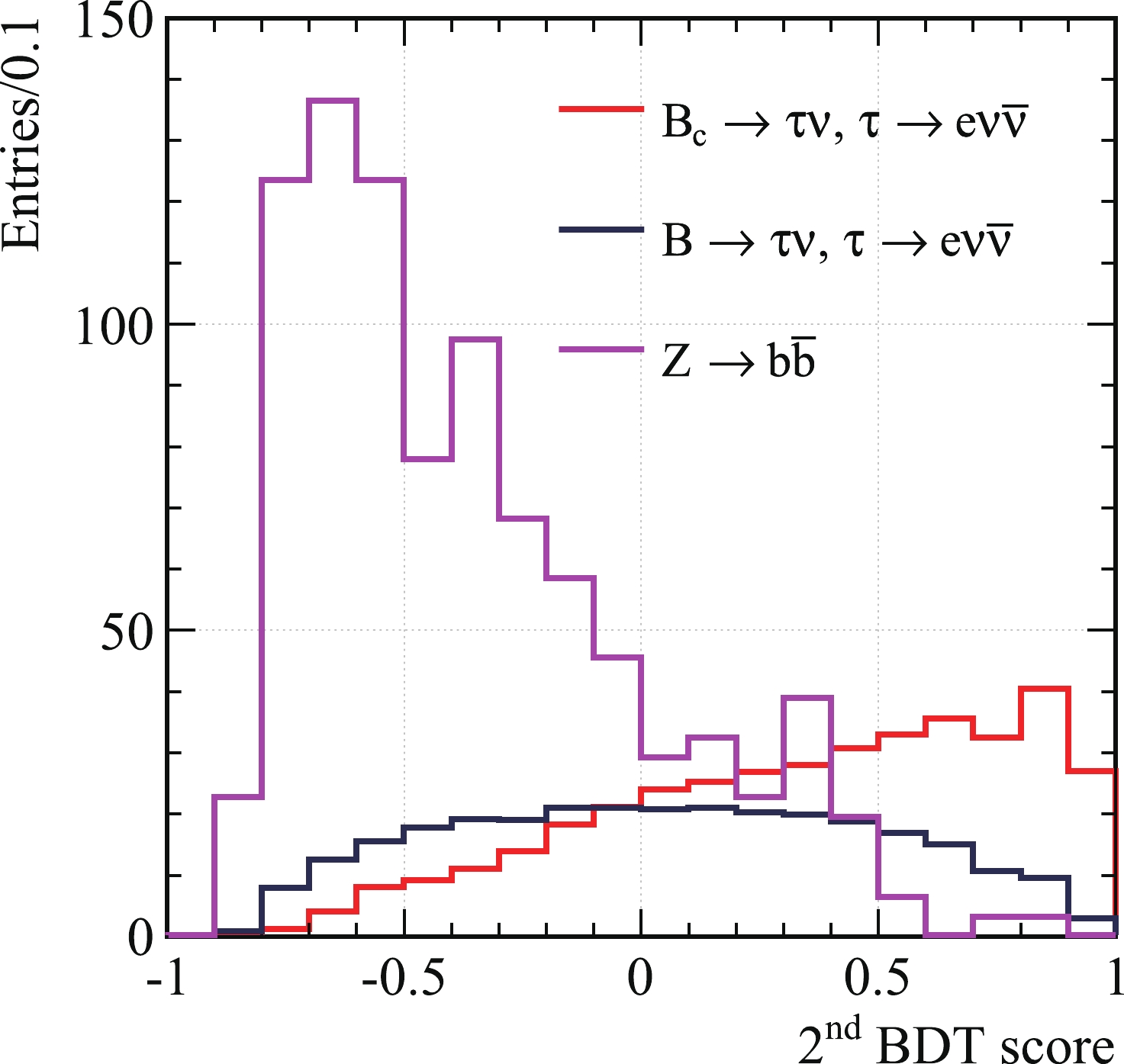
Figure 8. (color online) The second BDT score.
Now we can compute the relative accuracy of the signal strength:
$ \sigma(\mu)/\mu = \sqrt{N_S + N_B} / N_S \,, $

(16) where
$ N_S $ and$ N_B $ denote the numbers of signal and background events that pass all selection cuts, respectively. For the electron final states, we have$ \sigma(\mu_e)/\mu_e = 9.7 $ %. We can repeat the entire process for the muon final state. Here we will include the non-muon$ \tau $ decay channels in the second BDT, since the numbers of events are significantly larger. The results are shown in Table 2, and$ \sigma(\mu_{\mu})/\mu_{\mu} = 10.6 $ %. Combining the two final states, we have$ \sigma(\mu)/\mu = 7.2 $ %. It is now straightforward to calculate$ \sigma(\mu)/\mu $ for both$ B^+_c/B^+ \to \tau^+\nu_\tau $ at Tera-Z at various$ R_{B_c/B} $ . For the$ B \to \tau\nu, \tau \to e/\mu\nu\overline{\nu} $ analysis, all we need to do is repeat the second BDT after switching the signal and background status between it and the$ B_c $ . Figure 9 shows their relationship with$ R_{B_c/B} $ . Here, the yield$ N(B^\pm \to \tau^+\nu_\tau) $ is fixed at$ 1.3 \times 10^4 $ per one billion Z. The projected$ \sigma(\mu)/\mu $ s at Tera-Z are around$ {\cal{O}}(0.1) \sim {\cal{O}} $ (1)% level for both$ B^+_c \to \tau^+\nu_\tau $ and$ B^+ \to \tau^+\nu_\tau $ . At the$ R_{B_c/B} $ value given in Eq. (2), where the yield$ N(B^\pm_c \to \tau^+\nu_\tau) $ is around$ 3.6 \times 10^3 $ per one billion Z, we need around$ 10^9 $ Z boson decays to achieve five$ \sigma $ significance. In Sec. II we discussed the$ |V_{cb}| $ measurement, and with our current results we argue that the accuracy could reach up to$ {\cal{O}} $ (1)% level with certain improvements.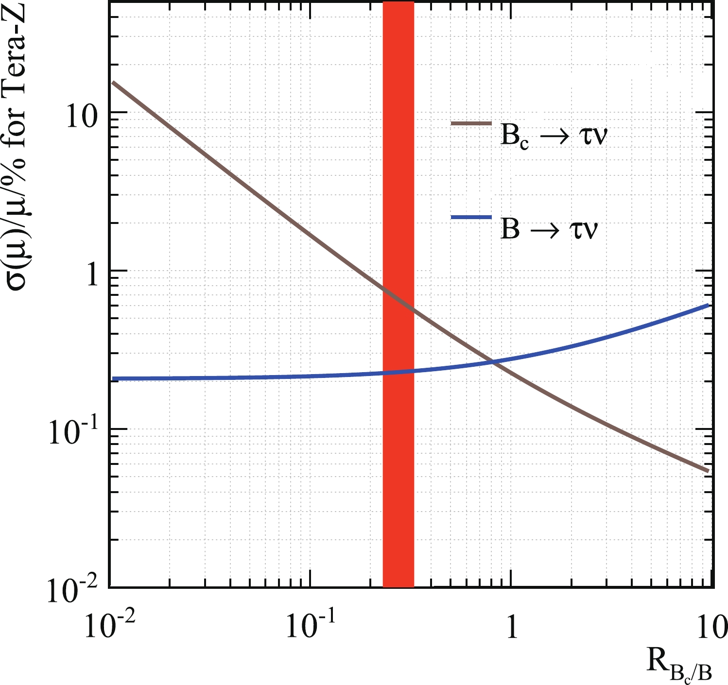
Figure 9. (color online)
$ \sigma(\mu)/\mu $ at Tera-Z versus$ R_{B_c/B} $ . The estimated range of$ R_{B_c/B} $ in Eq. (2) is shown in the red band. The actual uncertainty is larger, since we lack uncertainty for$ {\cal B}(Z \to B^\pm_cX) $ . -
As we have shown in Sec. II, based on the current results on NP in
$ b\to c\tau\nu $ ,$ \varGamma(B^+_c \to \tau^+\nu_\tau) $ tends to deviate from SM predictions, but the statistical importance is not significant. From Fig. 9, one can see that at the CEPC,$ \sigma(\mu)/\mu $ for$ B^+_c \to \tau^+\nu_\tau $ can reach about 1% level. This includes the constraint in both the production of$ B^+_c $ and the decay into$ \tau^+\nu_\tau $ . If the production mechanism is well understood, the result for$ \sigma(\mu)/\mu $ would also imply that the uncertainties in$ \varGamma(B^+_c \to \tau^+\nu_\tau) $ are reduced to the percent level. Furthermore, in the future one could also use$ {\cal B}(B_c^+ \to J/\psi\pi^+) $ as a calibration mode. In theory, lattice QCD can calculate the$ B_c \to J/\psi $ transition form factors while the perturbative contributions are well under control in perturbation theory.One can use such results for
$ \varGamma(B_c^+\to \tau^+\nu_\tau) $ to probe NP to a high precision. In Fig. 10, we show the constraints on$ {\rm{Re}}[C_{{\rm{V}}_2}] $ and$ {\rm{Im}}[C_{{\rm{V}}_2}] $ . If the central values in Eq. (9) remain the same while the uncertainty in$ \varGamma(B_c^+\to \tau^+\nu_\tau) $ is reduced to 1%, the allowed region for$ C_{{\rm{V}}_2} $ shrinks to the dark-blue regions, where the deviation from the SM is greatly enhanced.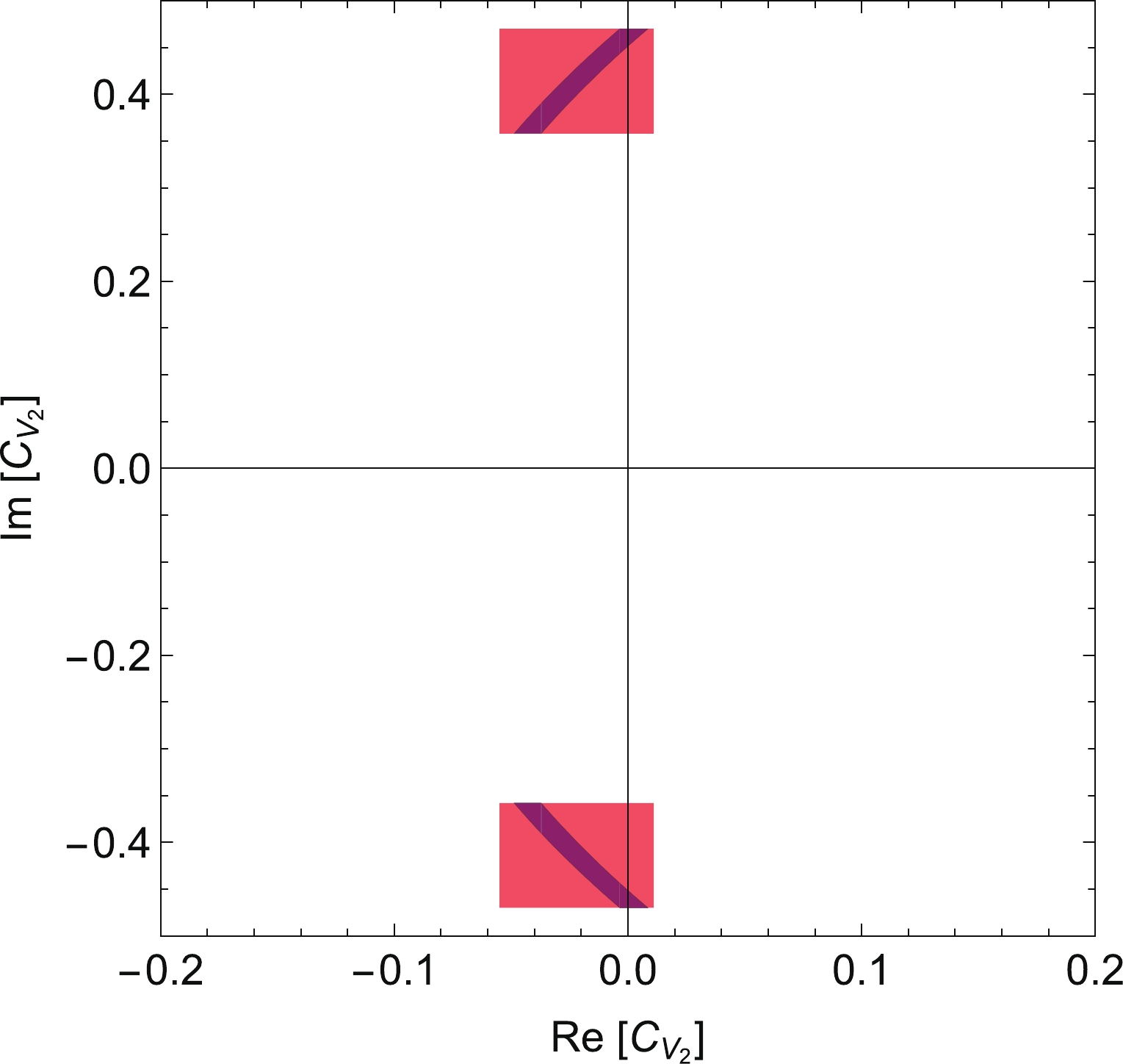
Figure 10. (color online) Constraints on the real and imaginary parts of
$ C_{V_2} $ . The red shaded area corresponds to the current constraints using available data on$ b\to c\tau\nu $ decays. If the central values in Eq. (9) remain while the uncertainty in$ \varGamma(B^+_c \to \tau^+\nu_\tau) $ is reduced to 1%, the allowed region for$ C_{V_2} $ shrinks to the dark-blue regions.Similar results can be obtained for the NP coefficients
${ C_{{\rm{S}}_1}} $ and${ C_{{\rm{S}}_2}} $ , but as we have demonstrated in Sec. II, both scenarios will induce dramatic changes to$ \varGamma(B_c^+\to \tau^+\nu_\tau) $ . These NP effects are so large that they would already be verified or ruled out before entering into the high-precision era of the CEPC. Thus it is less meaningful to present the constraints for these two coefficients. -
Nowadays, hunting for new physics beyond the Standard Model is a primary objective in particle physics. In this paper, we have first demonstrated that the decay
$ B^+_c \to \tau^+\nu_\tau $ provides a unique opportunity to probe new physics contributions, especially to the (pseudo)scalar interactions that exist in many popular models, such as the two-Higgs-doublet model and the leptoquark models.We then analyzed the decay
$ B^+_c \to \tau^+\nu_\tau, \tau^+ \to e^+/\mu^+\nu\overline{\nu} $ at the CEPC Z pole. We referred to the methods used in the L3 analysis [11] for the search for$ B^+ \to \tau^+\nu_\tau $ , which shares a similar event topology. The backgrounds under consideration are$ Z \to q\overline{q} $ and$ B^+ \to \tau^+\nu_\tau $ , as well as other$ \tau $ decay channels of$ B^+_c \to \tau^+\nu_\tau $ . We used a first stage cut chain to suppress most of the light-flavor backgrounds, and subsequently used a 2-stage BDT method to perform a fine-tuned multi-variable analysis. The first BDT separates heavy flavor backgrounds and the second BDT separates$ B^+ \to \tau^+\nu_\tau $ events. The current detector design and reconstruction algorithms provide excellent signal lepton reconstruction efficiency and purity, and do not pose significant constraints on the analysis. We have demonstrated that under current estimates for$ N(B^\pm_c \to \tau^\pm\nu_\tau) $ of around$ 3.6 \times 10^3 $ per one billion Z, we need around$ \sim10^9 $ Z decays to achieve five$ \sigma $ significance. The relative accuracy of the signal strength could reach around 1% level at Tera-Z. If the total$ B^+_c $ yield can be determined to$ {\cal{O}} $ (1%) level accuracy in the future,$ |V_{cb}| $ can also be expected to be measured to$ {\cal{O}} $ (1%) level of accuracy. Our theoretical analysis shows the channel has good potential for NP searches and could provide a significant constraint on NP related to the Wilson coefficient$ C_{{\rm{V}}_2} $ in Eq. (5). We also showed the projected signal strength accuracy for various signal event numbers for both$ B^+_c/B^+ \to \tau^+\nu_\tau $ . The results could be improved with a more exhaustive analysis, especially the inclusion of hadronic$ \tau $ decays and a larger sample of MC-simulated events.To summarize, we have demonstrated the CEPC's benchmark capability for the study of
$ B^+_c \to \tau^+\nu_\tau $ . The results show that the CEPC could provide a new opportunity to search for NP such as the 2HDM and LQ models, measure$ |V_{cb}| $ and test our understanding of QCD. -
We are in debt to Haibo Li, Yiming Li, and Jianchun Wang for useful discussion. We'd like to thank Chengdong Fu and Gang Li for their technical support. In addition, we want to thank Fenfen An for her early studies. We also acknowledge the Priority Academic Program Development for Jiangsu Higher Education Institutions (PAPD).
Analysis of Bc → τντ at CEPC
- Received Date: 2020-09-08
- Available Online: 2021-02-15
Abstract: Precise determination of the


 DownLoad: