


 Abstract
 HTML
HTML Reference
 Related
 PDF
PDF


-
One of the most impressive features of nuclear structures is band mixing at low energies. Several decades ago, Carchidi and colleagues [1, 2] developed generalized two-state model wave functions within the coexistence model for
$ 0^+ $ states in even-even nuclei. A linear combination of the basis states in the two-state model is common. Recently, it has been shown [3–8] that precise evidence exists for the presence of band mixing in medium mass nuclei such as those of Zr, Pd, Mo, Cd, Te, and Xe isotopes. Due to the large space configuration, shell-model calculations with multi particle-hole excitations are not simple. To determine the nuclear structure of band mixing in the collective valence shell and multi-particle-hole excitations, the interacting boson model (IBM) has been proposed [9, 10]. The mass region A$ \simeq $ 100 has been of considerable interest for features of the U(5) to SO(6) transition in even-even nuclei. This mass region is sensitive to patterns such as quantum phase transitions, band mixing, and shape coexistence configurations [11–13].Fortune, in Ref. [14], has determined the amount of mixing between the lowest two
$ 2^+ $ ,$ 4^+ $ , and$ 6^+ $ states in$ ^{72} $ Ge. In this region, he analyzed mixing between the first two$ 0^+ $ and$ 2^+ $ states in$ ^{96} $ Zr [15]. Small mixing pertains to small E0 strength in this nucleus. In heavy mass nuclei, the mixing configuration of members of the first two rotational bands in$ ^{152} $ Sm is apparent [16]. In this case, the lower basis-state band is more collective than the second band. This region exhibits a shape change from the spherical structure of the neutron closed shell nucleus to a rotational, deformed structure. Binary-reaction spectroscopy has provided a new understanding of the band crossing in$ ^{100} $ Mo [17] and of a coexistence configuration in the vibrational limit to a rotational limit [18, 19]. In recent studies, different isotopes have been applied to obtain nuclear structures such as mixed-symmetry states as well as band mixing in$ ^{94,96} $ Mo and shape coexistence in$ ^{98} $ Mo [20–24].The nuclear structures classified in different mass regions have been described by the usual IBM-1, with no distinction made between neutrons
$ N_\nu $ , protons$ N_\pi $ , Proton-Neutron IBM-2, E5, and X5 critical-point excitation and phase coexistence [25–28]. Unlike IBM-1, which is related to the fully symmetric states$ F = F_{\rm max} = (N_\pi+N_\nu)/2 $ , IBM-2 is related to the exchange and interaction of proton and neutron configurations in the band mixing of the wave function. We know that IBM-2 is often adopted in configuration mixing schemes. The states are called band mixing. In nuclear models, the coexistence mixing configuration (CMC) seems to work better due to the band mixing. The CMC calculations have been confirmed to be successful in explaining normal and intruder states that are related to IBM-1 and IBM-2. Though most CMCs have been examined in the IBM-2 framework, configuration mixing can also be analyzed in accordance with IBM-1, with no distinction between neutron-type and proton-type bosons, as shown in Refs. [29–31]. In the CMC, several terms play a role in explaining the band mixing instead of IBM-2. In other words, the CMC is another feature of IBM-2, which does not consider the proton and neutron interactions. Consequently, the CMC with different symmetry limits from the IBM can undoubtedly be of great help in understanding shape coexistence phenomena.The authors of Ref. [12] explicitly explored the degree of separation energy as a signature of coexisting shapes. Lesher et al. [24] reported several low-spin states as band mixing of a
$ (n, n^{\acute{}} \gamma ) $ reaction. In their calculations, the band mixing and coexistence configuration were performed between U(5) and O(6) limits.It may be that the coexistence configurations involve mixed states, as suggested recently by Thomas et al. [32], who used
$ \gamma\gamma $ angular correlation experiments to study spins, multipole mixing ratios, and collective E2 properties. They collected information on the deformation energy surface and mixed-symmetry state.Given this information and the conclusions from Refs. [9, 33–36] regarding analytic expressions and exact eigen energies between the spherical and
$ \gamma $ -soft shapes found by using the Bethe-ansatz within an infinite-dimensional Lie algebra, it would be helpful to describe the shape coexistence configuration and band mixing in$ ^{96,98} $ Mo. We thus followed the method of Refs. [9, 33, 34] and applied a simple two-state model to the energy spectra and electric transition rates in$ ^{96,98} $ Mo. The exact solution and band mixing configurations have recently been shown to be successful in reproducing the lowest state band and E2 matrix elements.It is preferable to work with the proton-neutron interacting model due to the interaction of protons with neutrons, as explained in Ref. [20]. The CMC calculation can be used to explore the normal 2p-0h proton configuration for U(5) vibrational nuclei and the three intruder phonons, with a 2p-4h or 4p-2h configuration across the Z = 40 sub-shell for O(6)
$ \gamma $ -soft nuclei. To this end, we used the same formalism and calculations via the SU(1,1) Lie algebra and SU(1,1) coherent states [9, 33, 37] for the lowest states of band mixing connecting the$ 0^{+} $ and$ 2^{+} $ states and the$ 4^{+} $ and$ 2^{+} $ states. -
IBM-1 and CMC are prominent phenomenological models for describing the mixing of low-lying collective states across an entire major shell. In our system, generators can be constructed in terms of l-boson operators as
$ S^{+}({l}) = \dfrac{1}{2}l^{\dagger}.l^{\dagger} $ for the creation operator,$ S^{-}({l}) = \dfrac{1}{2}{\tilde{l}}.{\tilde{l}} $ for the annihilation operator, and$ S^{0}({l}) = \dfrac{1}{2}\left(l^{\dagger}.{\tilde{l}}+ \dfrac{2l+1}{2}\right) $ for the number-conserving operator, with$ l = 0 $ for s bosons and$ l = 2 $ for d bosons [33, 34]. We use the theory of affine$ \widehat{SU(1,1)} $ algebraic techniques [33, 34], which determines the properties of energy spectra, mixing of states, and electric transition rates. By employing the generators of the affine$ \widehat{SU(1,1)} $ algebra in terms of l-boson operators, a solvable Hamiltonian is constructed for the transitional region between the vibrational and intruder configurations. The Hamiltonian can be written as$ \hat{H } = S_{0}^{+} S_{0}^{-}+ S_{1}^{0} $ by adding the second Casimir of$ \hat{C }_{2}(SO(2l+1))+ \hat{C }_{2}(SO(3)) $ for IBM-1 [33]. All details of the calculations can be found in Refs. [33, 34].$ \hat{H } = S_{0}^{+} S_{0}^{-}+ S_{1}^{0}+\hat{C }_{2}(SO(2l+1))+ \hat{C }_{2}(SO(3)). $

(1) In order to describe the CMC, we first define a typical consistent-Q Hamiltonian in the framework of the original IBM-1 as
$ \hat{H}_{CQ} = \epsilon_d\;\hat{n}_d-\kappa\;\hat{Q}(\chi)\cdot \hat{Q}(\chi), $

(2) where
$ \epsilon_d $ ,$ \kappa $ , and$ \chi \in [-\sqrt{7}/2,0] $ are real parameters of the model. Thus, a suitable Hamiltonian for describing the CMC may be written as [9]$ \hat{H} = \hat{P}(\triangle\;\hat{n}_s\;+\triangle\;\hat{n}_d+\hat{H_0}+m (S^++S^-\;))\;\hat{P}, $

(3) where
$ \hat{H_0} = \varepsilon_d\;\hat{n}_d+cC_2(O(5))+f \hat{L}\cdot\;\hat{L} $ is a U(5)-limit Hamiltonian; c and f are real parameters needed to remove the degeneracy in the level energies for a fixed number of d bosons,$ n_d $ , but with different$ \nu $ and L.$ \Delta $ is the energy needed to excite two more particles from the closed-shell, resulting in a configuration with two more particles and two more holes; it is taken to be a constant for simplicity when 2n-particles and 2n-hole excitations with n = 0, 1, 2, ... are considered. m is the mixing parameter under the projection operator of P in the CMC.The coexistence configuration has been found in Mo isotopes where the normal and intruder states were defined by U(5) and O(6) limits, respectively [38]. Suppose that the normal states (N bosons) with a vibrational limit and intruder states (N+2 bosons) with a rotational limit coexist and that they can interact and mix. In that case, the total lowest weight
$ \mid lw> $ wave function can be$ a\left|lw_{N}\right \rangle_{(g)}+ b\left|lw_{N+2}\right\rangle_{(e)} $ , where the subscripts g and e refer to the ground and excited bands, respectively, and$ \mid l'w'\rangle \equiv N, n_{d}, \nu, n_{\Delta}, L, M $ . We do not want to restrict band mixing to the$ n_{d} = N $ and$ n_{d} = N+2 $ states. Rather, this is an example of band mixing that can be extended to other states. We apply the mixing of several simple states to the transitions in the three apparent$ 0^{+} $ ,$ 2^{+} $ , and$ 4^{+} $ bands and the transitions of$ 0\leftrightarrow2 $ and$ 2\leftrightarrow4 $ in each nucleus. This mixing band configuration has been previously applied to several mass regions from light to heavy mass nuclei, for which evidence exists on the coexistence of different structures at low excitation energies. This simple approach attempts to extract the exact solution with high accuracy.Measurements of the reduced transition probabilities, B(E2;
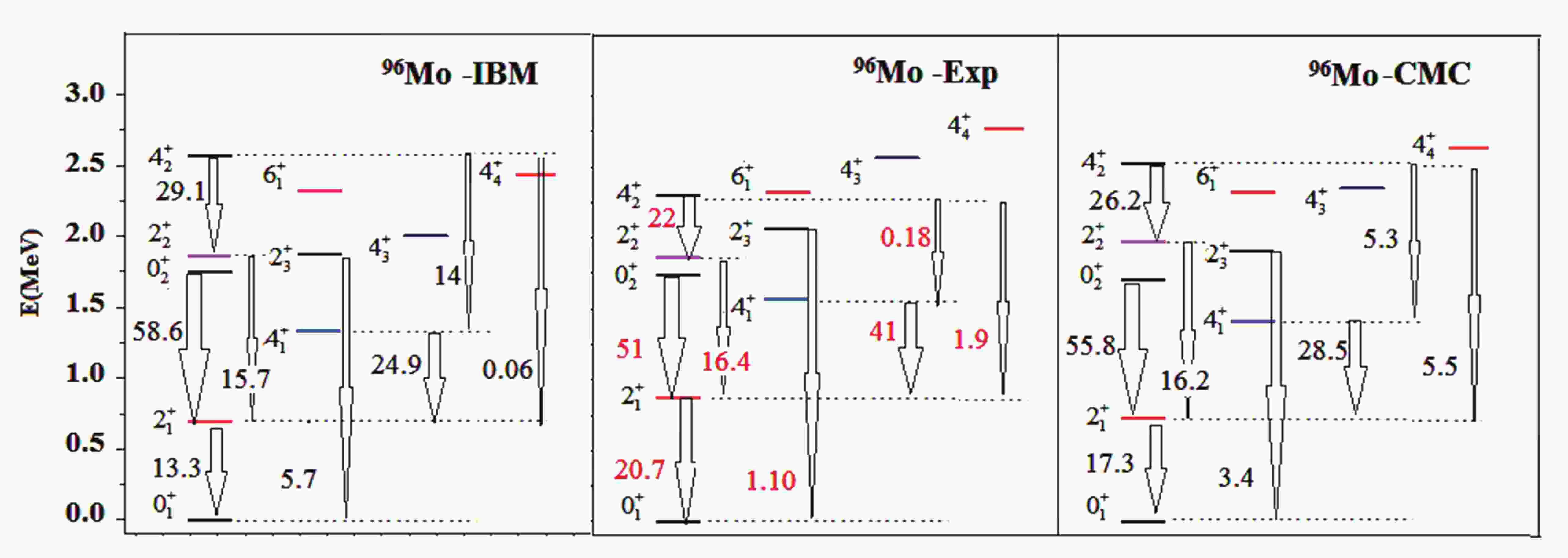
$ 4\rightarrow2 $ ) and B(E2;$ 2\rightarrow1 $ ) , and their ratio, R = B(E2;$ 4\rightarrow2)/B(E2; 2\rightarrow1 $ ), are good indicators of the phase transition and collectivity of a nucleus in this transitional region. The energy spectra and some partial transition rates of low-lying states related to band mixing in$ ^{96,98} $ Mo are plotted and compared in Figs. 1 and 2. From the value of the transition matrix elements and comparison with experimental data, CMC is better than IBM-1. That is, the results of CMC have higher accuracy, i.e., minimum$\left(\sigma =\left(\dfrac{1}{N_{\rm tot}}\sum\nolimits_{i,{\rm tot}} | E_{{\rm exp}(i)} - E_{\rm{cal}}(i){|}^2 \right)^{\frac{1}{2}}\right)$ values, when compared with the experimental data. In the mean root square,$ {{{N}}_{{\rm{tot}}}}$ is the number of energy states included in the extraction processes.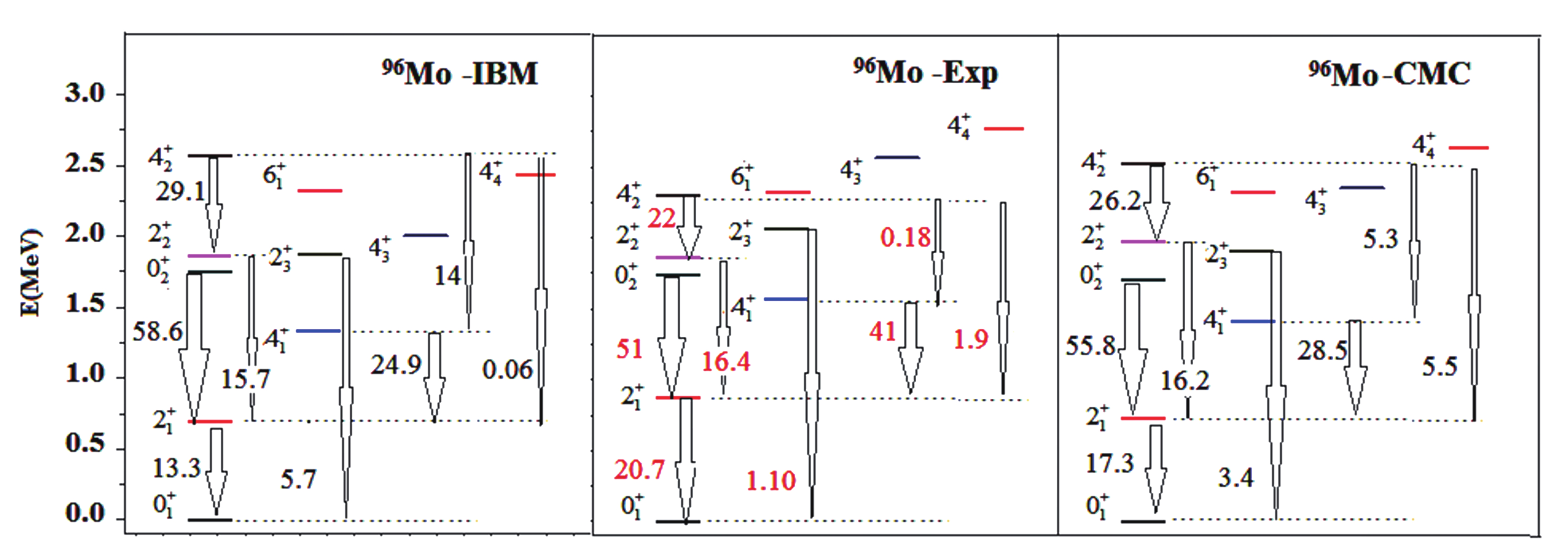
Figure 1. (color online) Energy spectra and E2 strengths for the lowest states in even-even
$ ^{96} $ Mo. The experimental data were taken from [39].
Figure 2. (color online) Energy spectra and E2 strengths for the lowest states in even-even
$ ^{98} $ Mo. The experimental data were taken from [40].To represent the band mixing, we introduce two bands, g and e, as in the Refs. [14, 15], with the
$ 0^{+} $ ,$ 2^{+} $ , and$ 4^{+} $ basis lowest state wave functions$ 0_g $ ,$ 0_e $ ;$ 2_g $ ,$ 2_e $ ; and$ 4_g $ ,$ 4_e $ , respectively. We define the lowest weight$ \mid lw\rangle $ state for the ground state and some excited states as$ \begin{aligned}[b] \left|lw\right\rangle_{(g.s.)}({}^AMo) =& a\left|lw\right\rangle_{(g)}+b\left|lw\right\rangle_{(e)}, \\ \left|lw\right\rangle_{(0_2^+)}({}^AMo) =& b\left|lw\right\rangle_{(g)}-a\left|lw\right\rangle_{(e)}, \end{aligned} $

(4) where the coefficients of a and b are the mixing amplitudes. These coefficients represent the mixing amplitudes for both the ground and excited states. Later, when mixing the potentials, we use
$ a_0b_0 $ ,$ a_2b_2 $ , and$ a_4b_4 $ for the ground and excited$ 0^+ $ ,$ 2^+ $ , and$ 4^+ $ states, respectively. We define the lowest weight state for the ground and excited states of the$ 2^{+} $ and$ 4^{+} $ bands, similar to Eq. (4). The lowest weight state of the mixing band should satisfy the relation$ S^{-} (s) |l'w'\rangle = 0, \quad S^{-} (d) |l'w'\rangle = 0 $ . To evaluate the strength of the matrix elements and energy spectra based on the affine SU(1,1) algebra, the eigenstates are considered as$ |k;\nu_{d}\nu_{s}n_\Delta LM \rangle = N S^{+}(x_{1})S^{+}(x_{2})S^{+}(x_{3})...S^{+}(x_{k})|l'w'\rangle, $

(5) where
$ \nu_{s} $ and$ \nu_{d} $ are seniority quantum numbers. To obtain the eigenstates of (1), the Fourier-Laurent expansion of the eigenstates of (1) can be investigated using the SU(1,1) generators$ S^{+}(x_{i}) $ in terms of unknown c-number parameters,$ x_i $ (roots of k pairs) with$ i = 1,2,...k $ , and$ S^{+}(x_{i}) = \frac {C_{s}}{1-C_{s}^{2} x_{i} } S^{+} (s)+\frac {C_{d}}{1-C_{d}^{2} x_{i} } S^{+} (d), $

(6) where
$ C_s $ and$ C_d $ are real control parameters. We thus obtain N as the normalization factor with$ N = \sqrt{\frac{1}{\left( \displaystyle\sum\limits_{i = n}^{k}{\dfrac{2{{C}_{s}}^{2}\left(k-n+\dfrac{1}{2}\left({{\nu }_{s}}+\dfrac{1}{2}\right)\right)}{(1-C_{s}^{2}{{x}_{k+1-n}})(1-C_{s}^{2}{{x}_{i}})}+\frac{2\left(k-n+\dfrac{1}{2}\left({{\nu }_{d}}+\dfrac{5}{2}\right)\right)}{(1-{{x}_{k+1-n}})(1-{{x}_{i}})}} \right)}}, $

(7) where we fix
$ C_{s} $ = [0, 1] and$ C_{d} $ = 1 in the phase transition.The author of Refs. [4, 15] followed a unique determination for the parameters of the two-state model. Here we instead develop an exact solution for the mixed states.
We can define the first set of eigenstates (called normal states in what follows), which are labeled with an additional quantum number
$ \zeta $ = 1 and are similar to those provided by the U(5) limit of the IBM without CMC, by SU(1,1) coherent states [9],$ \vert\zeta = 1,\vert lw\rangle = {\rm e}^{\alpha S_s^++\beta S_d^+}\;\vert lw\rangle. $

(8) Since the s-boson part and d-boson part of the Hamiltonian are separated, using the Hausdorff-Campbell relation, we use
$ \zeta = 1 $ for unmixed states and$ \zeta = 2 $ for excited mixed states. Details of the exact solutions have been presented in Refs. [9, 33, 34].The electric quadrupole operator is simply defined as
$\begin{aligned}[b] {T} _{ \mu}^{(E2)} =& q_{e2}\hat{P}_N [(s^{\dagger}\times \tilde{d} + d^{\dagger} \times \tilde{s})_{\mu}^{(2) }]\hat{P}_N\\&+q'_{e2}\hat{P} [(s^{\dagger}\times \tilde{d} + d^{\dagger} \times \tilde{s})_{\mu}^{(2) }]\hat{P},\end{aligned} $

(9) where
$ \hat{P}_N $ is the projection operator onto the configuration mixing without multiparticle-hole excitations. The reduced transition probability$ B(E2) $ is given by$ B(E2; \alpha _{i} L_{i} \rightarrow \alpha _{f} L_{f}) = \frac {|\langle \alpha _{f} L_{f} || T^{E2} || \alpha _{i} L_{i}\rangle |^{2} }{2L_{i}+1}, $

(10) where the reduced matrix element is defined in terms of the CG coefficient, and
$ \langle \alpha _{f} L_{f} || \hat{I} || \alpha _{i}L_{i}\rangle = \delta_{\alpha _{f},\alpha _{i}}\delta_{L_{f},L_{i}} $ with the unit identity operator$ \hat{I} $ .For the projection operator, we have
$ \hat P|N',{n_d},\nu ,{n_\Delta },L,M\rangle = \left\{ {\begin{array}{l} {|N',{n_d},\nu ,{n_\Delta },L,M\rangle }&{{\rm if}\;N' \geqslant N}\\ 0&{\rm otherwise} \end{array}} \right., $

(11) which keeps the operator effective only within the boson subspace by
$ [N]\oplus[N+2]\oplus[N+4]\oplus... $ mixed configurations.Here, we define the matrix elements
$ M_g $ and$ M_e $ connecting the$ 0^{+} $ and$ 2^{+} $ states and$ 4^{+} $ and$ 2^{+} $ states$ M_g = \left\langle0_g\left|E2\right|2_g\right\rangle, \quad \quad M_e = \left\langle0_e\left|E2\right|2_e\right\rangle, $

(12) and
$ M_g^{'} = \left\langle2_g\left|E2\right|4_g\right\rangle, \quad \quad M_e^{'} = \left\langle2_e\left|E2\right|4_e\right\rangle. $

(13) Furthermore, we assume that, for the band mixing of the ground and excited states, the g states are not connected to the e states by the E2 operator then the square of the electric transition amplitude. Thus,
$ M\;(E2;\;J_i\rightarrow J_f\;) $ , satisfying$ M\;^2(E2;\;J_i\rightarrow J_f\;) = (2J_i+1)B(E2;\;J_i\rightarrow J_f\;) $ . We report the reduced electric quadrupole rates for eight transitions, including the four connecting$ 0\leftrightarrow2 $ from$ M0-M3 $ and the four connecting$ 2\leftrightarrow4 $ from$ M4-M7 $ in$ ^{96} $ Mo. We also have five rates for the transitions connecting$ 0\leftrightarrow2 $ from$ M^{'}0-M^{'}4 $ and four for those connecting$ 2\leftrightarrow4 $ from$ M^{'}5-M^{'}8 $ in$ ^{98} $ Mo. The reduced E2 transitions are listed in Tables 1 and 2. For the convenience of subsequent discussion, we use the labels$ M0-M7 $ for$ ^{96} $ Mo and$ M^{'}0-M^{'}8 $ for$ ^{98} $ Mo.label initial final $ M(E2)_{\rm exp} $ 

$ M(E2)_{\rm IBM-1} $ 

$ M(E2)_{\rm CMC} $ 

$ M0 $ 

$ 2^{+}_{1} $ 

$ 0^{+}_{1} $ 

10.17 8.15 9.30 $ M1 $ 

$ 0^{+}_{2} $ 

$ 2^{+}_{1} $ 

7.14 7.65 7.46 $ M2 $ 

$ 2^{+}_{2} $ 

$ 2^{+}_{1} $ 

9.05 8.86 9.0 $ M3 $ 

$ 2^{+}_{3} $ 

$ 0^{+}_{1} $ 

2.34 5.33 4.12 $ M4 $ 

$ 4^{+}_{1} $ 

$ 2^{+}_{1} $ 

19.20 14.96 16.01 $ M5 $ 

$ 4^{+}_{2} $ 

$ 4^{+}_{1} $ 

1.27 11.22 6.90 $ M6 $ 

$ 4^{+}_{2} $ 

$ 2^{+}_{1} $ 

4.13 0.73 7.03 $ M7 $ 

$ 4^{+}_{2} $ 

$ 2^{+}_{2} $ 

14.07 16.18 15.35 Table 1. Experimental and theoretical values of
$ M(E2) $ (W.u.) connecting the$ 0^{+} $ and$ 2^{+} $ states from$ M0-M3 $ and$ 4^{+} $ and$ 2^{+} $ states from$ M4-M7 $ in$ ^{96} $ Mo.label initial final $ M^{'}(E2)_{\rm exp} $ 

$ M^{'}(E2)_{\rm IBM-1} $ 

$ M^{'}(E2)_{\rm CMC} $ 

$ M^{'}0 $ 

$ 2^{+}_{1} $ 

$ 0^{+}_{1} $ 

9.94 8.51 9.20 $ M^{'}1 $ 

$ 2^{+}_{2} $ 

$ 0^{+}_{2} $ 

3.39 5.14 4.36 $ M^{'}2 $ 

$ 2^{+}_{2} $ 

$ 0^{+}_{1} $ 

2.28 3.86 2.08 $ M^{'}3 $ 

$ 2^{+}_{3} $ 

$ 0^{+}_{2} $ 

6.0 4.0 5.73 $ M^{'}4 $ 

$ 2^{+}_{3} $ 

$ 0^{+}_{1} $ 

0.4 4.0 3.65 $ M^{'}5 $ 

$ 4^{+}_{1} $ 

$ 2^{+}_{1} $ 

19.51 17.33 18.97 $ M^{'}6 $ 

$ 4^{+}_{1} $ 

$ 2^{+}_{2} $ 

11.61 15.26 14.26 $ M^{'}7 $ 

$ 4^{+}_{2} $ 

$ 2^{+}_{1} $ 

unknown 7.22 5.36 $ M^{'}8 $ 

$ 4^{+}_{2} $ 

$ 2^{+}_{2} $ 

unknown 12.51 13.07 Table 2. Experimental and theoretical values of
$ M(E2) $ (W.u.) connecting the$ 0^{+} $ and$ 2^{+} $ states from$ M^{'}0-M^{'}4 $ and$ 4^{+} $ and$ 2^{+} $ states from$ M^{'}5-M^{'}8 $ in$ ^{98} $ Mo.To describe the band mixing in the nuclei, it might be helpful to apply simple two-state mixing with fewer fitting parameters. For our band mixing, we analyze the
$ 0\leftrightarrow2 $ and$ 2\leftrightarrow4 $ transitions separately, with the lowest weight states for$ ^{96} $ Mo and$ ^{98} $ Mo, and then compare the$ 2^{+} $ mixing obtained in the separate fits. Results for the$ 0\leftrightarrow2 $ and$ 2\leftrightarrow4 $ fits and a comparison with IBM-1 and CMC are listed in Table 1 for$ ^{96} $ Mo and Table 2 for$ ^{98} $ Mo. We obtain the coefficients of the lowest weight states for the mixing band by a fitting procedure. The amplitudes have physical meaning in that we can define the strength of the mixing using these values. When adjusting the parameters, we confine the amplitudes to [0-1] to clearly determine the strength of the mixing. We report the g and e amplitudes for the low lying states.Inspection shows that the experimental sum of
$ M^2 $ for$ ^{96} $ Mo is greater than the sum of$ M^{'}{^2} $ for$ ^{98} $ Mo. The sum of$ M^2 $ for connecting the$ 0^{+} $ and$ 2^{+} $ states for$ ^{96} $ Mo and the sum of$ M^{'}{^2} $ for the same states for$ ^{98} $ Mo are 241.76 and 151.64 Weiskopf units (W.u.), respectively.The sum of
$ M^2 $ for connecting the$ 2^{+} $ and$ 4^{+} $ states for$ ^{96} $ Mo and sum of$ M^{'}{^2} $ for the same states for$ ^{98} $ Mo are 585.26 and 515.43 (W.u.), respectively. The first and second$ 2^{+} $ state has high strength for both the$ 2^{+} $ and$ 0^{+} $ states. For example, the relevant E2 matrix elements$ M(E2) $ in$ ^{96} $ Mo for the transitions of$ 2^{+}_{1}\rightarrow 0^{+}_{1} $ and$ 2^{+}_{2}\rightarrow 2^{+}_{1} $ are 10.17 and 9.05, respectively. Moreover, the value of$ M^{'}(E2) $ in$ ^{98} $ Mo for the transitions of$ 2^{+}_{1}\rightarrow 0^{+}_{1} $ is 9.94. The results of our fitting for IBM-1 and CMC confirm this pattern. We can conclude, as has long been thought, that the first two$ 2^{+} $ states are maximally mixed.Based on variations of our calculations, we conclude that the IBM-1 sum is slightly smaller than the experimental one. Nevertheless, the CMC results are large, indicating too much deformation (and/or collectivity) in that calculation. We also note that the CMC sum is larger than that of IBM-1. The deviations that occur when connecting the
$ 2\leftrightarrow4 $ fits are shown in Figure. Some of the discrepancies of an extraction of the$ 2\leftrightarrow4 $ transitions refer to a shortage of experimental data for$ 4^{+}_{2}\rightarrow 2^{+}_{2} $ and$ 4^{+}_{2}\rightarrow 2^{+}_{1} $ in the fitting procedure of$ ^{98} $ Mo.Based on the value of B(E2) connecting the first and second
$ 4^{+} $ states to the first and second$ 2^{+} $ states [39, 40], it is clear that it is the$ 4^{+} $ state that should be included in the mixing. The experimental values of$ M(E2) $ in$ ^{96} $ Mo for the transitions of$ 4^{+}_{1}\rightarrow 2^{+}_{1} $ and$ 4^{+}_{2}\rightarrow 2^{+}_{2} $ are 19.20 and 14.07, respectively. The experimental values of$ M^{'}(E2) $ in$ ^{98} $ Mo for the transitions of$ 4^{+}_{1}\rightarrow 2^{+}_{1} $ and$ 4^{+}_{1}\rightarrow 2^{+}_{2} $ are 19.51 and 11.61, respectively. Unfortunately, there are no experimental data for the transitions of$ 4^{+}_{2}\rightarrow 2^{+}_{1} $ and$ 4^{+}_{2}\rightarrow 2^{+}_{2} $ , but we have calculated the IBM-1 and CMC for these transitions. It should be noted that the small size of M and$ M^{'} $ in our system is usually indicative of weak mixing and$ M_g\gg M_e $ .In the extraction procedure, connecting the
$ 0 \leftrightarrow 2 $ transitions, the E2 matrix elements of the g band are approximately 1.83 and 2.16 times greater than those of the e band for IBM-1 and CMC, respectively, in$ ^{96} $ Mo. Moreover, the E2 matrix elements of the g band for connecting the$ 2 \leftrightarrow 4 $ transitions in$ ^{96} $ Mo are greater than those of the e band by approximately 2.19 and 3.29 times for IBM-1 and CMC, respectively. Our results suggest that the basis-state transition matrix elements for the g bands are more significant than for the e bands. This also holds for$ ^{98} $ Mo. For connecting the$ 0 \leftrightarrow 2 $ transitions, the E2 matrix elements of the g band are approximately 2.30 and 3.09 times greater than those of the e band for IBM-1 and CMC, respectively, in$ ^{98} $ Mo. Furthermore, the E2 matrix elements of the g band for connecting the$ 2 \leftrightarrow 4 $ transitions in$ ^{98} $ Mo are approximately 2.07 and 2.37 times greater than those of the e band for IBM-1 and CMC, respectively. The conclusion is again that the lower basis-state band is slightly more collective for Mo isotopes. Comparing these extractions, we can conclude that the CMC results are better than those of IBM-1. Using the notation from Tables 1 and 2, we have some interesting results: the relation$ \sum_{}M_i^2 = M_g^2+M_e^2 $ is prominent for both connecting transitions. A comparison of these assumptions for$ \sum_{}M_i^2 $ is given in Figs. 3 and 4 for$ ^{96} $ Mo and$ ^{98} $ Mo. The values of Fits 1 and 2 are related to the calculation of IBM-1 and CMC, respectively. We can see that the fitted values of CMC are in good agreement with the experimental data.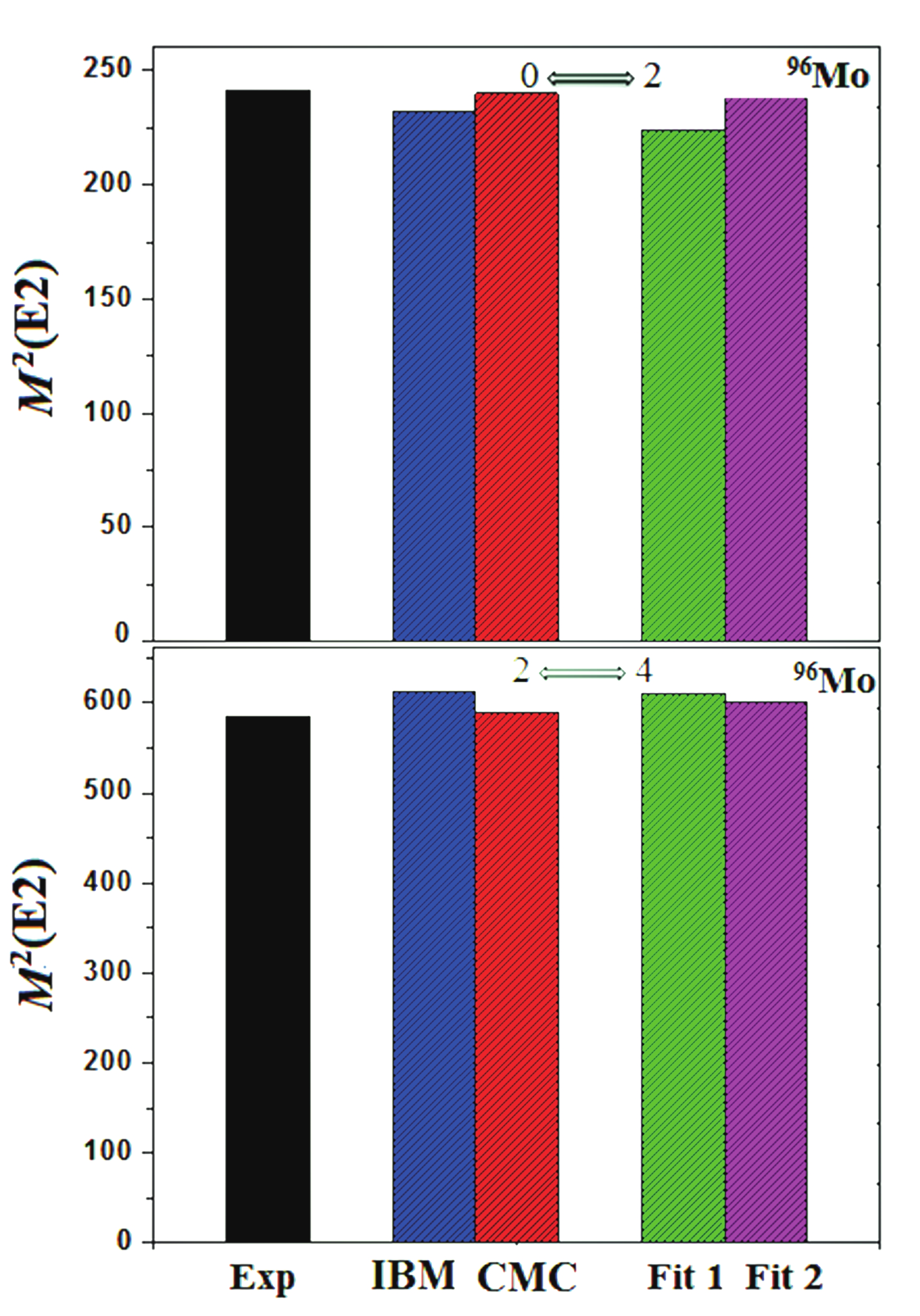

Figure 4. (color online) The same as Fig. 3 in
$ ^{98} $ Mo.The best fit results for the basis-state transition matrix elements connecting the
$ 0^{+} $ and$ 2^{+} $ states and$ 2^{+} $ and$ 4^{+} $ states in$ ^{96,98} $ Mo are shown in Tables 3-6. In both$ ^{96,98} $ Mo isotopes, the lower basis-state (g-band) is found to be somewhat more collective than the second state.parameter $ M_g $ 

$ M_e $ 

$ R=M_e/M_g $ 

value fit 1 13.37 7.28 0.54 value fit 2 14.07 6.49 0.46 Table 3. Best fit results for connecting the
$ 0^{+} $ and$ 2^{+} $ states in$ ^{96} $ Mo.parameter $M_g$ 

$M_e$ 

$R=M_e/M_g$ 

value fit 1 22.51 10.26 0.45 value fit 2 23.22 7.05 0.30 Table 4. Bets fit results for connecting the
$2^{+}$ and$4^{+}$ states in$^{96}$ Mo.parameter $M^{'}_g$ 

$M^{'}_e$ 

$R^{'}=M^{'}_e/M^{'}_g$ 

value fit 1 11.07 4.81 0.43 value fit 2 11.81 3.82 0.32 Table 5. Best fit results for connecting the
$0^{+}$ and$2^{+}$ states in$^{98}$ Mo.parameter $ M^{'}_g $ 

$ M^{'}_e $ 

$ R^{'}=M^{'}_e/M^{'}_g $ 

value fit 1 24.53 11.83 0.48 value fit 2 25.46 10.70 0.42 Table 6. Best fit results for connecting the
$ 2^{+} $ and$ 4^{+} $ states in$ ^{98} $ Mo.This solution has
$ R = M_e/M_g $ = 0.45, which is almost the same as the ratio$ R^{'} = M^{'}_e/M^{'}_g $ = 0.48 for the$ 2 \leftrightarrow 4 $ transitions in IBM-1. The solution also has$ R = M_e/M_g $ = 0.30, which is similar to$ R^{'} = M^{'}_e/M^{'}_g $ = 0.42 for the$ 2 \leftrightarrow 4 $ transitions in CMC. Good agreement with CMC is also noted in this case. Nevertheless, this trend does not hold for the$ 0 \leftrightarrow2 $ transitions. This may indicate that the$ 0^{+} $ state should not be included in good band mixing.Recently, considerable attention has been directed to investigating band mixing based on the coexistence model [41]. The authors of [41] proposed a two-state model containing band mixing, which could be used as a signature of collectivity. Some interesting structures are investigated in the paper, and it is shown that the variation of the matrix elements can modify the structure of the nuclei. In this region, the authors found a two-state mixing model in the lowest two
$ 0^+ $ ,$ 2^+ $ , and$ 4^+ $ states of$ ^{42} $ Ca. The excited band was found to be more collective than the ground band in$ ^{42} $ Ca [41]. In our case, the resulting structural information consists of the extracted values of the basis-state transition matrix elements for the$ (g) $ and$ (e) $ bands. The small size of the resulting$ M_e $ reveals that the upper$ 2^{+} $ basis state, especially in the case of$ 2^{+}_{3} $ , is nearly spherical with no strong E2 to$ 0^{+} $ state ($ 2^{+}_{3}\rightarrow 0^{+}_{1} = 1.10 $ ) in$ ^{96} $ Mo and ($ 2^{+}_{3}\rightarrow 0^{+}_{1} = 0.032 $ ) in$ ^{98} $ Mo. This suggests that this state has a spherical shape and that it can be treated as an intruder state. In particular, it means that there are coexistence configurations associated with these states. In our work, we also report the collectivity of states using the algebraic model, and this solvable model confirms the coexistence configuration. Therefore, investigation of the band mixing in this structure reveals that the nuclear models presented here can be utilized for other signatures of coexistence configurations. Each physical ground$ (g) $ and excited$ (e) $ state can be represented as a linear combination of basis states. From the coefficients in Eq. (4), we find that the basis state$ 0_g $ is lower in energy than$ 0_e $ , and the pattern is the same for higher J. Therefore, the ground band is below the excited band. The extracted values of the basis-state in the transition matrix elements, which emerge from the analysis of Eqs. (12) and (13), indicate that$ M_g $ and$ M^{'}_g $ are larger than$ M_e $ and$ M^{'}_e $ for connecting the$ 0\leftrightarrow 2 $ and$ 2\leftrightarrow 4 $ transitions in$ ^{96,98} $ Mo. Then, the conclusion is that the lower basis-state band is slightly more collective. According to an analysis of the IBM and CMC configurations, the dominance of the basis-state g increases as the angular momentum J in the lower state increases. The ratios$ M_e/M_g $ and$ M^{'}_e/M^{'}_g $ are remarkably constant in$ ^{98} $ Mo. Furthermore, the absolute values of the basis-state transition matrix elements ($ M_g, M^{'}_g, M_e $ , and$ M^{'}_e $ ) support the earlier remark that$ ^{96} $ Mo is slightly more collective than$ ^{98} $ Mo.The energy spectra and relevant E2 matrix elements that arise from the fits for IBM and CMC are presented and are compared to the experimental values. The values of M and
$ M^{'} $ are provided in the figures. These values indicate that, as discussed above, the CMC analysis agrees much better with the experimental data than do the IBM predictions. A comparison of the matrix elements and the absolute values of$ M_g $ and$ M_e $ suggests that$ ^{96} $ Mo is slightly more collective than$ ^{98} $ Mo. It is evident that the CMC calculations are good agreement with the present data. We now present our numerical results for the best fit related to the CMC calculations in order to illustrate and compare the mixing amplitudes and mixing potentials in$ ^{96} $ Mo and$ ^{98} $ Mo. The mixing amplitudes and mixing potentials derived from the best fit are listed in Table 7. We note that the strength of mixing for the g band in the lower state increases as the angular momentum J increases from 0 to 4. The comparison is clear in the table. By solving and analyzing the band mixing and fitting procedure for the coefficients, we find that the coefficients of the ground states are larger than the coefficients of excited states, indicating that the basis state of the ground states is lower in energy than the excited states. This behavior is even more pronounced for higher angular momenta: the coefficients$ J_{g}>J_{e} $ for the$ 0^{+} $ up to the$ 4^{+} $ state. We therefore know that the g band is below the e band. We have also seen that the extracted values of the matrix elements for$ ^{96} $ Mo and$ ^{98} $ Mo indicate that$ M_g $ and$ M^{'}_g $ are larger than$ M_e $ and$ M^{'}_e $ . The conclusion is that the lower basis-state band is slightly more collective.J $ ^{96} $ Mo g amplitude

$ ^{96} $ Mo V/keV

$ ^{98} $ Mo g amplitude

$ ^{98} $ Mo V/keV

0 0.50 315.70 0.43 164.12 2 0.77 249.32 0.69 191.31 4 0.89 172.01 0.86 108.18 Table 7. Comparison of the mixing amplitudes and mixing potentials in
$ ^{96} $ Mo and$ ^{98} $ Mo.Next, we focus on an important indicator of band mixing, the mixing potential, which can be defined based on the level spacing. The level spacing of the low lying states is essential for describing the band mixing. The spacing of the
$ 0^{+} $ ,$ 2^{+} $ , and$ 4^{+} $ states can be combined with the mixing amplitudes to obtain the matrix elements responsible for the mixing. Thus, in each nucleus, the mixing potentials between the$ 0^{+} $ ,$ 2^{+} $ , and$ 4^{+} $ bands are$ V_{0} = a_{0}b_{0} \Delta E_{2} $ ,$ V_{2} = a_{2}b_{2} \Delta E_{2} $ , and$ V_{4} = a_{4}b_{4} \Delta E_{4} $ , respectively. The comparisons are listed in Table 7. From the interaction matrix elements in a two-state model, we can learn the collectivity of the basis states. We find the wave-function amplitudes by analyzing the IBM and CMC models. The mixing amplitudes arise from the extraction of coefficients from Eq. (4). The spacings (energy separation) of the physical states for the J =$ 0^{+} $ ,$ 2^{+} $ , and$ 4^{+} $ states are useful for determining the mixing potentials. For instance, for$ 0^{+} $ , we have$ V_{0} = a_{0}b_{0} \Delta E_{2} $ , where$ \Delta E_{2} $ is the energy difference in the nucleus between the excited$ 0^{+} $ state and the ground state. We have similar expressions for the other angular momentum values. We neglect the negative values of the mixing potentials because physically, we select positive$ a_0 $ and$ b_0 $ in the wave function, thereby dismissing solutions for negative values. The same scheme can be extended to a combination of two$ 2^{+} $ states or two$ 4^{+} $ states. Thus far, in our discussion, an inspection of the mixing amplitudes and mixing potentials for both nuclei indicates that the two$ 2^{+} $ states are almost maximally mixed. Important information is contained in the mixing amplitudes and mixing potentials that arise from the analysis. Based on the analysis and the results in Table 7, we find that the mixing potential for$ ^{96} $ Mo is higher than for$ ^{98} $ Mo. We can conclude that in IBM-1, we do not have a projection operator in the Hamiltonian when compared with CMC. By adding a U(5) limit term and applying the projection operator, we are able to consider the band mixing in the Mo isotopes. One of the main criteria for selecting the appropriate model in our work is the results for the energy spectra and E2 transition. We also achieve good agreement between the variation of$ M(E2 $ ) and$ M^{'}(E2) $ with the experimental data. We can conclude that the results for two-state mixing based on the mixing model are better than the results based on IBM for the band mixing of Mo isotopes. -
We applied the lowest weight
$ lw $ two-state mixing model to the partial$ 0^{+} $ ,$ 2^{+} $ , and$ 4^{+} $ states of Mo isotopes and the matrix elements connecting them and compared it with nuclear models. The models are satisfactory for$ ^{96,98} $ Mo. The results indicate that the lower basis-state band is slightly more collective in both nuclei. The simple numerical approach presented in this paper opens up ways of understanding band mixing and coexistence configurations in the framework of the interacting boson approximation, i.e., CMC. The CMC calculations in the two-state mixing model reproduce the experimental data very well, providing insight into the mixing model between the lowest states. The results of the fitting indicate that the$ 0^{+} $ states are barely mixed, whereas the$ 2^{+} $ and$ 4^{+} $ states exhibit a high level mixing.In summary, we propose a novel theoretical two-state mixing based on a solvable model. From the numerical results produced by the interacting model, we find that this nuclear model can be an exceptional tool for describing the structure of band mixing. The main characteristics of the proposed structure, such as the energy spectra, transition probabilities, and other degrees of freedom, can be finely paraphrased by the interacting models.
Band mixing in 96,98Mo isotopes
- Received Date: 2020-07-02
- Available Online: 2021-02-15
Abstract: We use the two lowest weight states to fit E2 strengths connecting the


 DownLoad: