


 Abstract
 HTML
HTML Reference
 Related
 PDF
PDF


-
The first gravitational waves (GWs) were directly detected from the coalescence of binary black holes (BBHs) [1-8] by Advanced LIGO [9] and Virgo [10]. The recent experimental precision satisfies the requirement of general relativity theory, but the observational precision of GWs also leaves the window for alternative theories of gravity open [11]. In addition, the Event Horizon Telescope (EHT) collaboration recently released the first shadow image of a supermassive BH M87 [12, 13] in the galaxy. These results prove the existence of BHs in the universe, thus giving birth to a new era in the astronomy of astrophysical compact objects [14]. The interaction between two BHs can be conditionally divided into three phases: the inspiral phase [15], the merger phase [16], and the ringdown stage [17]. The portion of the GW signal associated with single BH oscillations is referred to as the ringdown phase, as the perturbed BH rings down, akin to a struck bell. The ringdown phase is the brief oscillation stage before the newly formed BH reaches its final stable state. The damping times and frequencies associated with a given BH are known as quasinormal modes (QNMs) [18]. Therefore, QNMs play a central role in the final stage, the ringdown phase, in the coalescence of BBHs [19-23].
In addition, BHs are nonlinear solutions to a highly nonlinear theory. It is always a difficult task to study their dynamics. The perturbation method is an effective tool to study the interaction between a BH and a basic test field. The study of BH perturbation started with Regge and Wheeler's [24] analysis of the perturbation of an axisymmetric gravitational field. Subsequently, Zerilli [25-27] studied polar symmetric perturbation. The BH perturbations were then systematically summarized in Chandrasekhar’s monograph [28]. A disturbed BH can be considered a dissipative system, and the perturbation has a discrete spectrum. As a consequence, QNM frequencies are complex numbers that also give the damping of the oscillations. The imaginary part of the frequencies represents the decay of the amplitude, and the real part corresponds to the oscillations of the perturbations. The decay time scale and oscillation frequency only depend on the spacetime background of the BH, independent of the initial disturbance. Because specific black holes have specific QNMs, they can accurately reflect the spacetime properties of BHs. This is graphically known as the characteristic sound of a BH, which has become a powerful tool to reveal the intrinsic properties of BHs. A good review of QNM theory can be found in [17, 18, 29, 30].
The mass, angular momentum, and charge of a BH can be determined by detecting the quasinormal frequencies and damping rates. QNMs can also be used to test the no-hair theorem and quantization of black holes [31, 32]. In addition, in gauge/gravity duality theory, there is a connection between QNMs and the poles of propagators in dual field theory, which is why physicists use it as a tool to study strongly coupled gauge theory (or holography) [33, 34]. Therefore, much attention has been given to modified theories of gravity.
In this paper, charged BHs in the Born-Infeld gravity are investigated. In 1930, born and Infeld proposed the nonlinear theory of electrodynamics and obtained the self-energy of a finite point charge in a nonlinear system [35]. The main motivation is to observe it occurring in D-branes and open superstrings. The low energy efficiency of open superstrings leads to Born-Infeld-type action [36]. Along with the development of superstring theory, the dynamics of some super-gravity soliton solution D-branes [37] are controlled by the interaction of Born-field action. Later, Garcia et al. obtained the Born-Infeld black hole solution [38], which has been extended to a nonlinear charged BH in general relativity, characterized by spacetime dimension n, mass M, charge Q, and nonlinear parameter
$ \beta $ . The major goal of our research in this article is to explore the physical characteristics of Born-Infeld BHs, where the spacetimes are perturbed and the QNMs generated are probed by the perturbation. Most research on the QNMs of Born-Infeld BHs has focused on scalar fields, electromagnetic fields, and gravitational field perturbations (that is, fields with integer spin). Fernando [39] calculated the gravitational perturbation of a charged BH under the Born-Infeld gravity. Liu et al. [40] studied the QNMs of the scalar field interacting with the electromagnetic field of the Born-Infeld AdS BH. To make the study more complete, based on the frame in high-dimensional spherically symmetric BHs [41, 42], we study the spacetime structure and the QNMs for massive and massless Dirac fields of Born-Infeld BHs. Using the WKB method, the effect of the dimension of spacetime n, charge Q, and multipole numbers$ |k| $ on the QNMs of Born-Infeld BHs is studied. Specially, the dynamic evolution of the Dirac perturbation fields in Born-Infeld spacetime is investigated using the finite difference method. The results show that the quasinormal behavior of Born-Infeld BHs depends on the dimension of spacetime n.The structure of this article is as follows: Section 2 explains the research background of the paper, which is mostly based on the QNMs under Dirac field perturbation. We study the stability of the Born-Infeld BH with the finite difference method in Section 3. In addition, we utilize the WKB method to calculate the QNMs numerically in Section 4, including two parts: Part A, where QNMs for massless fields are calculated; and Part B, in which the QNMs of Born-Infeld BHs are analyzed for the massive case. In the last section, the important consequences and expectations are revealed.
-
The general action describing Born-Infeld interaction in a
$ (n+1) $ -dimensional ($ n \geqslant 3 $ ) background without the cosmological constant$ \Lambda $ has the form [41-44]$ S = \int {\rm d}^{n+1}x\sqrt{-g}\left(\frac{R}{16\pi G}+L(F)\right), $

(1) where R is the scalar curvature, and the Born-Infeld
$ L(F) $ part of the action is decomposed to$ L(F) = 4\beta^{2}\left(1-\sqrt{1+\frac{F^{\mu\nu}F_{\mu\nu}}{2\beta^{2}}}\right ). $

(2) Here,
$ L(F) $ is a function of the electrodynamic field strength$ F_{\mu \nu} $ .$ \beta $ is a Born-Infeld parameter with dimensions of$ {\rm length}^{-(n+1)/2} $ . For simplicity, let us assume$ 16\pi G = 1 $ . In the limit$ \beta\rightarrow\infty $ , the Born-Infeld$ L(F) $ tends to be Maxwell's electrodynamics with$ -F^2 $ , and$ L(F) $ is$ L(F) = -F^{\mu\nu}F_{\mu\nu}+{\cal O}(F^{4}). $

(3) By changing the action of gauge field
$ A_{\mu} $ and metric field$ g_{\mu\nu} $ , the equations of motion and Einstein equations of an electromagnetic field can be derived$ \partial_{\mu}\left (\frac{\sqrt{-g}F^{\mu\nu}}{\sqrt{1+\dfrac{F^{\mu\nu}F_{\mu\nu}}{2\beta^{2}}}}\right ) = 0, $

(4) $ {R}_{\mu\nu}-\frac{1}{2}{R}g_{\mu\nu} = \frac{1}{2}g_{\mu\nu}L(F)+ \frac{2F_{\mu \alpha}F^{\; \alpha}_{\nu}}{\sqrt{1+\dfrac{F^{\mu\nu}F_{\mu\nu}}{2\beta^{2}}}}. $

(5) Assuming metric ansatz is in the form
$ {\rm d}s^{2} = -f(r){\rm d}t^{2}+\frac{1}{f(r)}{\rm d}r^{2}+ R^{2}(r)h_{ij}{\rm d}x^{i}{\rm d}x^{j}, $

(6) $ h_{ij} $ is a function of coordinates$ x^{i} $ . It spans a hypersurface whose curvature in$ (n-1) $ -dimensions is the scalar curvature$ (n-1)(n-2)k $ .$ f(r) $ and$ R(r) $ are two functions of r. For the metric (6), the non-vanishing components of the Ricci tensor are obtained as [45],$ {R}^{t}_{t} = -\frac{f''}{2} - (n-1)\frac{f'R'}{2R}, $

(7) $ {R}^{r}_{r} = -\frac{f''}{2}-(n-1)\frac{f'R'}{2R}-(n-1)\frac{fR''}{R}, $

(8) $ {R}^{i}_{j} = \left( \frac{n-2}{R^2}k -\frac{1}{(n-1)R^{n-1}}[f(R^{n-1})']'\right)\delta^{i}_{j}. $

(9) This is the derivative of a prime with respect to the coordinate r.
Regarding
$ F^{rt} $ , setting$ F^{\mu\nu} $ equal to$ 0 $ satisfies the class of solutions to Eq. (4), which yields$ F^{rt} = \frac{\sqrt{(n-1)(n-2)}\beta q}{\sqrt{2\beta^{2}R^{2n-2}+(n-1)(n-2)q^{2}}}, $

(10) where q is an integral constant associated with the electrodynamic charge. With the electric charge defined by
$Q = \dfrac{1}{4\pi} \int \ ^*F {\rm d}\Omega$ , we have$ Q = \frac{\sqrt{(n-1)(n-2)}\omega_{n-1}} {4\pi\sqrt{2}}q, $

(11) where
$ \omega_{n-1} $ is the volume of the hypersurface with curvature defined as$h_{ij}{\rm d}x^i{\rm d}x^j$ . There is$ F^{rt} $ in the$ \beta $ limit, as$ F^{rt} \sim \dfrac{q}{r^{n-1}} $ . The electric field is finite at$ r = 0 $ . The cosmological constant is redefined as$ \Lambda = 0 $ , and solving equation (6) yields$ \begin{split} f(r) =& k -\frac{m}{r^{n-2}} +\left( \frac{4\beta^2r^2}{n(n-1)} \right) \\ &-\frac{2\sqrt{2} \beta}{(n-1)r^{n-2}}\int \sqrt{2\beta^2r^{2n-2} +(n-1)(n-2)q^2 }{\rm d}r. \end{split}$

(12) For
$ k = 1 $ , the integral in (12) can be represented in terms of hypergeometric functions,$ \begin{split} f(r) =& 1-\frac{m}{r^{n-2}}+\left(\frac{4\beta^{2} r^{2}}{n(n-1)}\right) \\ &-\frac{2\sqrt{2}\beta}{n(n-1)r^{n-3}}\sqrt{2\beta^{2}r^{2n-2}+(n-1)(n-2)q^{2}} \\ &+\frac{2(n-1)q^{2}}{nr^{2n-4} } \ _2F_{1}\bigg[\frac{n-2}{2(n-1)},\frac{1}{2}, \frac{3n-4}{2(n-1)}, \\ & -\frac{(n-1)(n-2)q^{2}}{2\beta^{2}r^{2n-2}}\bigg]. \end{split}$

(13) Here, m is an integral constant that is dependent on the configured ADM mass M. This is given by
$ M = (n-1)\omega_{n-1}m. $

(14) The analytic function within
$ |z| <1 $ can be parsed to the full z plane. Therefore,$ _2F_1(a,b,c,z) $ is a single-valued analytic function that expands along the real number line in the z plane [45]. For$ |z| <1 $ ,$ _2F_1(a,b,c,z) $ has a convergent series expansion. This gives$ f(r) = 1 - {m\over{r^{n-2}}} + {q^2\over{r^{2n-4}}} - {(n-1)(n-2)^2 q^4\over{8 \beta^2 (3n -4)r^{4n-6}}}, $

(15) and when
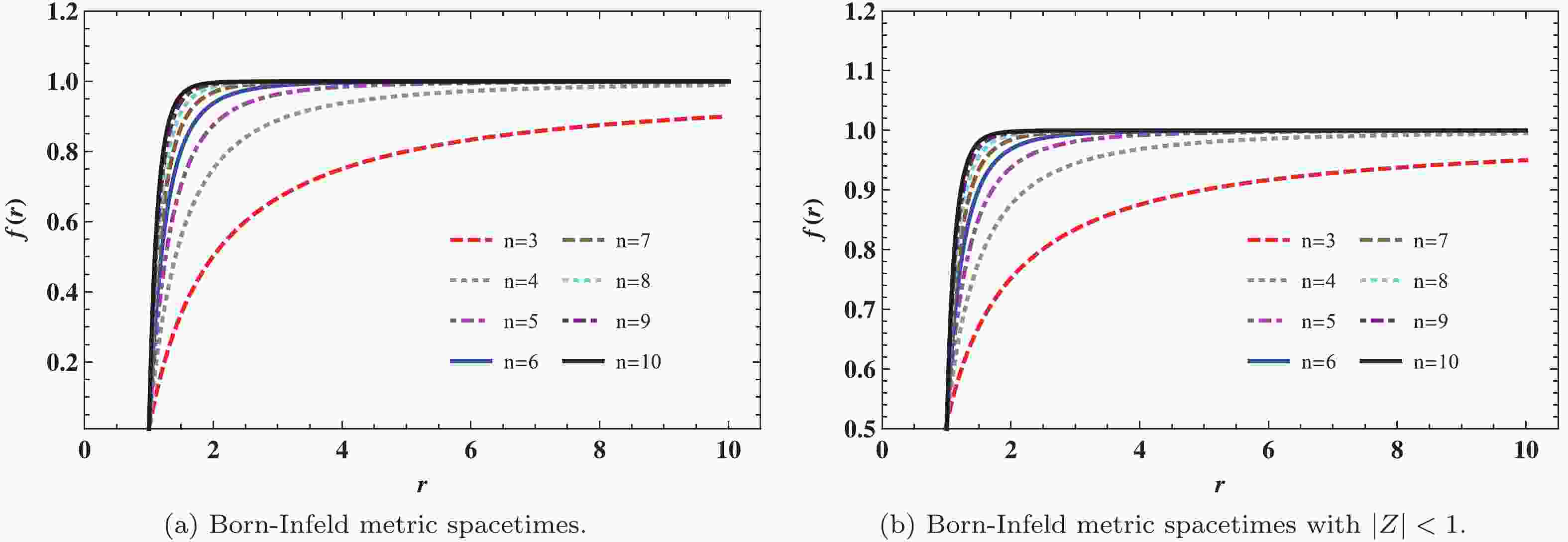
$ \beta \rightarrow \infty $ and$ n = 3 $ , the function$ f(r) $ describes Maxwell's electrodynamics for a Reissner-Norström (RN) BH [46, 47]. These are described in Table 1. Meanwhile, the spacetime structures of Born-Infeld BHs are exhibited in Fig. 1(a) and Fig. 1(b) ($ |z| <1 $ ). For asymptotically flat spacetime, the spacetime of Born-Infeld goes flat at infinity faster with increasing spacetime dimension n.${\rm{EBI}}\;{\rm{BH}}$ 

$f(r)= 1-\dfrac{m}{r^{n-2} }+\dfrac{4{\beta}^2r^2}{n(n-1)} -{ {\dfrac{2{\sqrt2}\beta}{(n-1)r^{n-2} }{\displaystyle\int{\sqrt{2{\beta}^2 r^{2n-2}+(n-1)(n-2)q^2} }{\rm d}r} } }$ 

$|z<1|$ 

$f(r) = 1 - \dfrac{m}{r^{n-2} } + \dfrac{q^2}{r^{2n-4} } - \dfrac{(n-1)(n-2)^2 q^4}{8 \beta^2 (3n -4)r^{4n-6} }$ 

$|z<1|$ ,

$\beta \rightarrow \infty$ 

$f(r) = 1 - \dfrac{m}{{r^{n-2} } } + \dfrac{q^2}{{r^{2n-4} } }$ 

$|z<1|$ ,

$\beta \rightarrow \infty$ ,

$n=3$ 

$f(r)_{RN} = 1 -\dfrac{m}{r}+ \dfrac{q^2}{{r^{2} } }$ 


Figure 1. (color online) Structures of the Born-Infeld metric function
$f(r)$ with different spacetime dimensions n: (from top to bottom:$n=3, 4, 5, 6, 7, 8, 9, 10$ ) (a) Born-Infeld metric spacetimes with$M=1$ ,$Q=0.1$ ,$b=0.1$ , and$r_+=1$ . (b) Born-Infeld metric spacetimes with$|z|<1$ ,$M=1$ ,$Q=0.1$ ,$b=0.1$ , and$r_+=1$ . -
The general equation for a massive Dirac spinor field in high-dimensional spacetime can be expressed as [50, 51]
$ \left[\gamma^{\mu}D_{\mu}+\frac{m}{\hbar}\right]\Psi = 0, \qquad \mu = t, r, \theta, \phi,x^{\eta},\cdots, {x}^{n+1}, $

(16) where
$ {x}^{n+1} $ are extra-dimensional coordinates,$ D_{\mu} = \partial_{\mu}+\frac{i}{2}{\Gamma^{\alpha}\,_{\mu}}^{\beta}\Pi_{\alpha\beta}, $

(17) where
$ \Pi_{\alpha\beta} = \dfrac{i}{4}[\gamma^{a},\gamma^{b}] $ and$ \Gamma_{\mu} = \dfrac{1}{8}[\gamma^{a},\gamma^{b}]e_{a}^{\nu}e_{b\nu;\mu} $ is a spin connection; the gamma matrices satisfy the condition that,$ \{\gamma^{\mu}, \gamma^{\nu}\} = 2g^{\mu\nu}I, $

(18) so the spinor wave function
$ \Psi $ in Eq. (16) can be written as$ \Psi = \left[ \begin{array}{c} A_{(m/2) \times 1}(t,r,\theta,\phi,x^{\eta},\cdots x^{n+1}) \\ B_{(m/2) \times 1}(t,r,\theta,\phi,x^{\eta},\cdots x^{n+1}) \\ \\ \end{array}\right] {\rm e}^{(-{\rm i}\omega t)S(t,r,\theta,\phi,x^{\eta},\cdots x^{n+1})} , $

(19) and the solution form of a statically spherically symmetric BH is given by Eq. (6)
$ e_{\nu}^{a} = {\rm diag}(f(r)^{1/2},f(r)^{-1/2},r,r\sin \theta, x^{\eta}, \cdots, x^{n+1}). $

(20) where
$ f(r) $ represents the Born-Infeld spacetime function listed in Table 1. The Dirac spinor can be written as,$ \Psi = f(r)^{-1/4}\Phi, $

(21) for higher-dimensional spacetime, the Dirac equation simplifies to
$ \left[\frac{1}{f}\left(\frac{\partial S}{\partial t}\right)+f\left(\frac{\partial S}{\partial r}\right)+g^{\theta\theta}\left(\frac{\partial S}{\partial \theta}\right) +g^{\phi\phi}\left(\frac{\partial S}{\partial \phi}\right)+g^{\eta\eta}\left(\frac{\partial S}{\partial x^{\eta}}\right)+ \cdots+g^{x^{n+1}x^{n+1}}\left(\frac{\partial S}{\partial x^{n+1}}\right)+m\right]\Phi = 0. $

(22) Wave functions must be defined separately as follows [52, 53].
$ \begin{split}&\Phi(t,r,\theta,\phi, x^{\eta}, \cdots, x^{n+1}) = \\&\quad\left( \begin{array}{c} \dfrac{iG^{\pm}(r)}{r}\varphi^{\pm}_{jm}(\theta,\phi) H(x^{\eta}, \cdots, x^{n+1})\\ \dfrac{F^{\pm}(r)}{r}\varphi^{\mp}_{jm}(\theta,\phi)H (x^{\eta}, \cdots, x^{n+1})\\ \end{array}\right) {\rm e}^{-{\rm i}\omega t}, \end{split}$

(23) and
$ \varphi^{+}_{jm} = \left( \begin{array}{c} \sqrt{\dfrac{l+1/2+m}{2l+1}}Y^{m-1/2}_{l} \\ \sqrt{\dfrac{l+1/2-m}{2l+1}}Y^{m+1/2}_{l} \\ \end{array} \right) \; \; \; \left({\rm{for}}\; j = l+\frac{1}{2}\right), $

(24) $ \varphi^{-}_{jm} = \left( \begin{array}{c} \sqrt{\dfrac{l+1/2-m}{2l+1}}Y^{m-1/2}_{l} \\ -\sqrt{\dfrac{l+1/2+m}{2l+1}}Y^{m+1/2}_{l} \\ \end{array} \right) \; \; \; \left({\rm{for}}\; j = l-\frac{1}{2}\right). $

(25) Radial functions (
$ G^{\pm} $ and$ F^{\pm} $ ) are considered. Eq. (22) is rewritten as$\begin{split}& \frac{{\rm d}}{{{\rm d}{r_*}}}\left( {\begin{array}{*{20}{c}} {{F^ \pm }}\\ {{G^ \pm }} \end{array}} \right) - \sqrt {f(r)} \left( {\begin{array}{*{20}{c}} {{k_ \pm }/r}&m\\ m&{ - {k_ \pm }/r} \end{array}} \right)\left( {\begin{array}{*{20}{c}} {{F^ \pm }}\\ {{G^ \pm }} \end{array}} \right) =\\&\quad \left( {\begin{array}{*{20}{c}} 0&{ - \omega }\\ \omega &0 \end{array}} \right)\left( {\begin{array}{*{20}{c}} {{F^ \pm }}\\ {{G^ \pm }} \end{array}} \right),\end{split}$

(26) where
${\rm d}/{\rm d}r_{*} = f(r){\rm d}/{\rm d}r$ . Let us proceed with some transformation of$ F^{\pm} $ and$ G^{\pm} $ [50],$ \left( {\begin{array}{*{20}{c}} {{{\hat F}^ \pm }}\\ {{{\hat G}^ \pm }} \end{array}} \right) = \left( {\begin{array}{*{20}{c}} {\sin \dfrac{\theta }{2}}&{\cos \dfrac{\theta }{2}}\\ {\cos \dfrac{\theta }{2}}&{ - \sin \dfrac{\theta }{2}} \end{array}} \right)\left( {\begin{array}{*{20}{c}} {{F^ \pm }}\\ {{G^ \pm }} \end{array}} \right), $

(27) where
$ \theta = \tan^{-1}(mr/|k|) $ . Introducing$ \hat{r}_{*} = r_{*}+ \tan^{-1} $ $(mr/|k|)/2\omega $ into Eq. (26), then$ \frac{{\rm d}}{{{\rm d}{{\hat r}_*}}}\left( {\begin{array}{*{20}{c}} {{{\hat F}^ \pm }}\\ {{{\hat G}^ \pm }} \end{array}} \right) + {W_ \pm }\left( {\begin{array}{*{20}{c}} { - {{\hat F}^ \pm }}\\ {{{\hat G}^ \pm }} \end{array}} \right) = \omega \left( {\begin{array}{*{20}{c}} {{{\hat G}^ \pm }}\\ { - {{\hat F}^ \pm }} \end{array}} \right),$

(28) where
$ W_{\pm} = \frac{\sqrt{f(r)\left(\dfrac{k_{\pm}^{2}}{r^{2}}+m^{2}\right)}}{1+\dfrac{f(r)m|k_{\pm}|}{2\omega(k_{\pm}^{2}+m^{2}r^{2})}}, $

(29) and
$ \frac{\rm d}{{\rm d}\hat{r}_{*}} = \frac{f(r)}{1+\dfrac{m|k_{\pm}|f(r)}{2\omega(k^{2}+m^{2}r^{2})}}\frac{\rm d}{{\rm d}r}. $

(30) The following derivation radial functions can be written as
$ \left(-\frac{{\rm d}^{2}}{{\rm d}\hat{r}^{2}_{*}}+\bar{V}_{\pm}\right)\hat{F}^{\pm} = \omega^{2}\hat{F}^{\pm}, $

(31) $ \left(-\frac{{\rm d}^{2}}{{\rm d}\hat{r}^{2}_{*}}+\tilde{V}_{\pm}\right)\hat{G}^{\pm} = \omega^{2}\hat{G}^{\pm}, $

(32) where
$ {\bar{V}}_{\pm} = \frac{{\rm d}W_{\pm}}{{\rm d}\hat{r}_{*}}+W^{2}_{\pm}, $

(33) and
$ \tilde{V}_{\pm} = -\frac{{\rm d}W_{\pm}}{{\rm d}\hat{r}_{*}}+W^{2}_{\pm}. $

(34) Here,
$ k_\pm $ is the number associated with the angular momentum quantum number l:$ k_{-} = -l $ for$ j = l-1/2 $ and$ k_{+} = l+1 $ for$ j = l+1/2 $ . In the following context, we only consider$ j = l-1/2 $ . Moreover, in spherically symmetric EBI spacetime, Dirac particles and antiparticles have the same QNMs. Therefore, the radial function$ \hat{F}^- $ can represent all the physics of Dirac field evolution. -
In this section, the QNM frequency is calculated, so the properties of the effective potential need to be determined. In the massless case,
$ \hat{F}^- $ was chosen as an example, thus$ \left(-\frac{{\rm d}^{2}}{{\rm d}\hat{r}^{2}_{*}}+V\right)\hat{F}^{-} = \omega^{2}\hat{F}^{-}, $

(35) where
$ V = \tilde{V}_{-}|_{m = 0} = -\frac{{\rm d}W_{-}}{{\rm d}\hat{r}_{*}}+W^{2}_{-}, $

(36) and
$ W_{-} = \sqrt{f(r)}\frac{|k_{-}|}{r}. $

(37) By simplifying the symbols, the '
$ - $ ' subscripts and superscripts of the rest are removed.$ r_+ = 1 $ is used.To calculate the QNM frequency of a BH, the properties of the potential function
$ V(r) $ are first considered. The Dirac effective potential of a Born-Infeld BH is in the form of a barrier, where$ V(r) $ depends on$ |k| $ , the spacetime dimension n, the Born-Infeld parameter b, and the charge Q. Fig. 2(a) shows the variation of the potential function$ V(r) $ with spacetime dimension n for Born-Infeld BHs under massless Dirac field perturbation. As seen in Fig. 2(a), the peak value of the barrier increases as the spacetime dimension n increases. Meanwhile, as shown in Fig. 2(b), as$ |k| $ increases, the peak value of the barrier also increases. From Fig. 2(b), we can find the position of the respective peaks. Similarly, the potential function of a Born-Infeld BH ($ |z|<1 $ ) has the same property, where slight differences are primarily caused by the hyperfunction
Figure 2. (color online) Behavior of Born-Infeld BH potential under massless condition: (a) different values of n (from top to bottom:
$n=3, 4, 5, 6, 7, 8, 9, 10$ ). (b) different values of$|k|$ (from top to bottom:$|k|=1, 2, 3, 4, 5$ ).$ r_{\max}(|k|\longrightarrow \infty )\longrightarrow 1.34, $

(38) and for a Born-Infeld BH
$ |z|<1 $ $ r_{\max}(|k|\longrightarrow \infty )\longrightarrow 1.26. $

(39) To numerically calculate the quasinormal mode frequencies of Born-Infeld BHs, we adopt the WKB approximation developed by Schutz, Will, and Iyer [54-56]. The values for different spacetime dimensions n are listed in Table 2, Table 3, and Table 4, where M is the mass of a Born-Infeld BH, Q is the electric charge, N is the overtone number,
$ |k| $ is related to angular quantum number values, and b is the Born-Infeld parameter. Here, we focus on the spacetime dimension n in the fundamental mode ($ N = 0 $ ) is focused. When$ \beta \rightarrow \infty $ and$ n = 3 $ , the Born-Infeld BH returns to a RN BH, and we compare the results in Born-Infeld BHs with those in RN BHs. The results indicate that$ {\rm{Re}}(\omega) $ and$ |{\rm{Im}}(\omega)| $ both increase as the spacetime dimension n increases. This result shows that for QNMs with higher spacetime dimensions, the rate of decay is accelerating compared with that of the low-dimensional ones. In addition,$ {\rm{Re}}(\omega) $ of the frequencies increases as the angular momentum number$ |k| $ increases with the same spacetime dimension n. However, the magnitude of the imaginary part$ |{\rm{Im}}(\omega)| $ is the opposite. Furthermore,$ {\rm{Re}}(\omega) $ and$ |{\rm{Im}}(\omega)| $ both increase significantly with increasing charge Q while$ |k| $ is constant. The results show that the damping of QNMs is affected by the amount of charge Q. In addition, gravitational perturbations of Born-Infeld BHs are studied in Ref. [39]. The QNM for the gravitational perturbations are computed also using the WKB method. It is interesting to note that although we chose a different range of parameters to calculate, we came to a consistent conclusion: for a Born-Infeld BH, when the charge increases, the imaginary part of the QNM continues to increase.$ n$ 

$|k|=3$ 

$|k|=4$ 

$|k|=5$ 

$RN$ 

$1.1557700139-0.1930619944i$ 

$1.5450184302-0.1929736171i$ 

$1.9335494699-0.1929352414i$ 

$3$ 

$1.1557037495-0.1931330986i$ 

$1.5449228497-0.1930424512i$ 

$1.9334264288-0.1930029746i$ 

$4$ 

$1.4824206993-0.3539002011i$ 

$1.9890849201-0.3535923516i$ 

$2.4935519194-0.3534612524i$ 

$5$ 

$1.6729838527-0.4947724401i$ 

$2.2548474671-0.4941886172i$ 

$2.8325512794-0.4939338712i$ 

$6$ 

$1.7963573716-0.6211054727i$ 

$2.4337539125-0.6203121349i$ 

$3.0645571714-0.6199625719i$ 

$7$ 

$1.8786688941-0.7359672425i$ 

$2.5607045617-0.7351652681i$ 

$3.2331497017-0.7348392792i$ 

$8$ 

$1.9324691882-0.8412210141i$ 

$2.6527294372-0.8407288004i$ 

$3.3597024024-0.8406414492i$ 

$9$ 

$1.9645121204-0.9380346977i$ 

$2.7192730919-0.9382670792i$ 

$3.4561830939-0.9387290357i$ 

$10$ 

$1.9786190819-1.0271463776i$ 

$2.7659881744-1.0285930212i$ 

$3.5298731019-1.0300078509i$ 

Table 2. Fundamental modes (
$N=0$ ,$r_{+}=1$ ,$b=0.1$ ,$Q=0.1$ ) of Dirac perturbations calculated by WKB method.n $|k|=3$ 

$|k|=4$ 

$|k|=5$ 

$RN$ 

$1.1807745781-0.1942520945i$ 

$1.5783039151-0.1941684492i$ 

$1.9751230049-0.1941320692i$ 

$3$ 

$1.1794987143-0.1951524435i$ 

$1.5765856643-0.1950532893i$ 

$1.9729713815-0.1950103782i$ 

$4$ 

$1.4936465475-0.3542072399i$ 

$2.0037367019-0.3538282015i$ 

$2.5117056128-0.3536702111i$ 

$5$ 

$1.6802097464-0.4945933092i$ 

$2.2638019281-0.4937606109i$ 

$2.8434200769-0.4934126781i$ 

$6$ 

$1.8021141106-0.6211467539i$ 

$2.4402161621-0.6197529004i$ 

$3.0720960321-0.6191715201i$ 

$7$ 

$1.8841584999-0.7368298925i$ 

$2.5660317057-0.7348615376i$ 

$3.2389749155-0.7340604371i$ 

$8$ 

$1.9384906269-0.8434959842i$ 

$2.6576702111-0.8410511909i$ 

$3.3646369485-0.8401125704i$ 

$9$ 

$1.9717294392-0.9423033713i$ 

$2.7243442984-0.9396110763i$ 

$3.4607270372-0.9386947312i$ 

$10$ 

$1.9786190819-1.0271463776i$ 

$2.7659881744-1.0285930212i$ 

$3.5298731019-1.0300078509i$ 

Table 3. Fundamental modes (
$N=0$ ,$r_{+}=1$ ,$b=0.1$ ,$Q=0.2$ ) of Dirac perturbations calculated by WKB method.n $|k|=3$ 

$|k|=4$ 

$|k|=5$ 

$RN$ 

$1.2284548139-0.1958292714i$ 

$1.6417685092-0.1957578811i$ 

$2.0543857019-0.1957267574i$ 

$3$ 

$1.2209047995-0.1995406409i$ 

$1.6318195877-0.1994576319i$ 

$2.0420288092-0.1994219029i$ 

$4$ 

$1.5110577791-0.3554398962i$ 

$2.0268844985-0.3551501808i$ 

$2.5405977577-0.3550318873i$ 

$5$ 

$1.6900627387-0.4942823704i$ 

$2.2768365497-0.4936848267i$ 

$2.8596374603-0.4934462438i$ 

$6$ 

$1.8085145254-0.6197325828i$ 

$2.4486792201-0.6187835582i$ 

$3.0825990887-0.6184289584i$ 

$7$ 

$1.8886219035-0.7344391294i$ 

$2.5719915869-0.7331381699i$ 

$3.2463865219-0.7327316406i$ 

$8$ 

$1.9417248012-0.8402141691i$ 

$2.6620585696-0.8385721119i$ 

$3.3701583101-0.8382343667i$ 

$9$ 

$1.9741818898-0.9383165293i$ 

$2.7276327314-0.9363307495i$ 

$3.4649741076-0.9362292839i$ 

$10$ 

$1.9897433647-1.0296336759i$ 

$2.7740734939-1.0272752331i$ 

$3.5376946367-1.0276151146i$ 

Table 4. Fundamental modes (
$N=0$ ,$r_{+}=1$ ,$b=0.1$ ,$Q=0.3$ ) of Dirac perturbations calculated by WKB method. -
Here, we use the finite difference method [57, 58] to illustrate the dynamic evolution of Born-Infeld BHs. We study the ringing of BH spacetimes, which can directly reflect the (in)stability of Born-Infeld BHs in the temporal evolution images containing all frequencies. Hence, using a numerical integration scheme [59], Eq. (28) can be expressed in light-cone coordinates:
$ \omega G^{\pm} = -\frac{f(r){\rm d}F^{\pm}}{{\rm d}r}+\sqrt{f(r)}\frac{k}{r}F^{\pm}+m\sqrt{f(r)}G^{\pm}, $

(40) $ \omega F^{\pm} = \frac{f(r){\rm d}G^{\pm}}{{\rm d}r}+\sqrt{f(r)}\frac{k}{r}G^{\pm}-m\sqrt{f(r)}F^{\pm}. $

(41) Multiplying both sides by
$ \omega $ , Eq. (40) and Eq. (41) are rewritten as$ \omega^{2} G^{\pm} \!\!=\!\! -\frac{\!f\!(r){\rm d}(\omega F^{\pm})}{{\rm d}r}\!\!+\!\!\sqrt{f(r)}\frac{k}{r}(\omega F^{\pm})\!+\!m\sqrt{f(r)}(\omega G^{\pm}), $

(42) $ \omega^{2} F^{\pm} \!\!=\!\! \frac{f(r){\rm d}(\omega G^{\pm})}{{\rm d}r}\!\!+\!\!\sqrt{f(r)}\frac{k}{r}(\omega G^{\pm})\!-\!m\sqrt{f(r)}(\omega F^{\pm}). $

(43) Putting Eqs. (40) and (41) into Eqs. (42) and (43),
$ \begin{split} \frac{m\sqrt{f}}{2}f'F^{\pm} =& f^{2}G''^{\pm}+ff'G'^{\pm}\\&+\left[\frac{kf'}{2r}\sqrt{f}-\frac{k^{2}}{r^{2}}f- \frac{k}{r^{2}}f^{3/2}+\omega^{2}-m^{2}f\right]G^{\pm}; \\ \frac{m\sqrt{f}}{2}f'G^{\pm} =& f^{2}F''^{\pm}+ff'F'^{\pm}\\&+\left[-\frac{kf'}{2r}\sqrt{f}-\frac{k^{2}}{r^{2}}f+ \frac{k}{r^{2}}f^{3/2}+\omega^{2}-m^{2}f\right]F^{\pm}. \end{split}$

(44) Here,
$ ' $ denotes$ \partial/\partial r $ ,$ \omega^{2} = -\partial^{2}/\partial^{2} t $ .$ (t,r) \rightarrow (\mu,\nu) $ is applied, where$ \mu = t-r_{*},\nu = t+r_{*} $ , yielding$ \frac{\partial}{\partial r} = \frac{1}{f}\left(\frac{\partial}{\partial \nu}-\frac{\partial}{\partial \mu}\right),\; \; \; \; \; \; \frac{\partial}{\partial t} = \frac{\partial}{\partial \nu}+\frac{\partial}{\partial \mu}. $

(45) $ F^{\pm}(\mu,\nu) $ and$ G^{\pm}(\mu,\nu) $ are deduced from Eq. (44), which can be integrated using the finite difference method [60, 61]. In Fig. 3 and Fig. 4, the plus '$ + $ ' and minus '$ - $ ' signs of$ F^{\pm}(\mu,\nu) $ are unified to be F.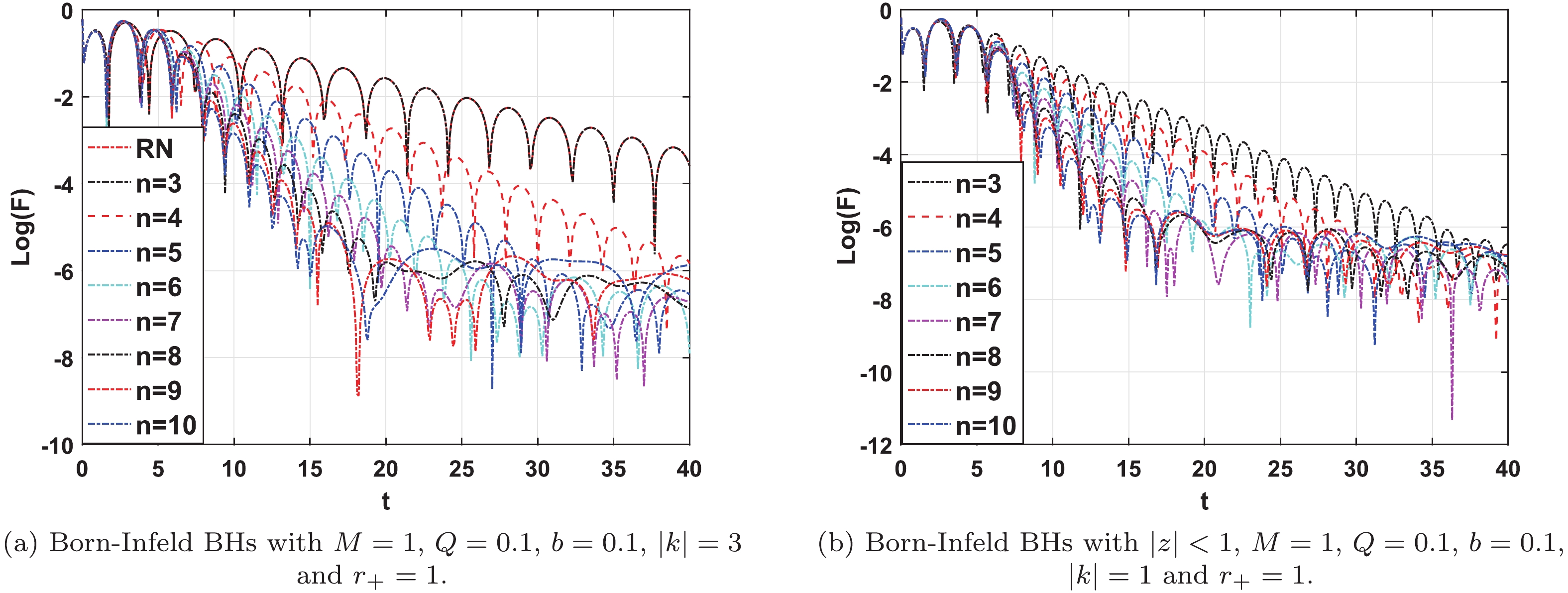
Figure 3. (color online) Dynamic evolution of Born-Infeld BHs with varying spacetime dimensions n (from top to bottom:
$n=3, 4, 5, 6, 7, 8, 9, 10$ ): (a) Born-Infeld BHs with$M=1$ ,$Q=0.1$ ,$b=0.1$ ,$|k|=3$ and$r_+=1$ . (b) Born-Infeld BHs with$|z|<1$ ,$M=1$ ,$Q=0.1$ ,$b=0.1$ ,$|k|=1$ and$r_+=1$ .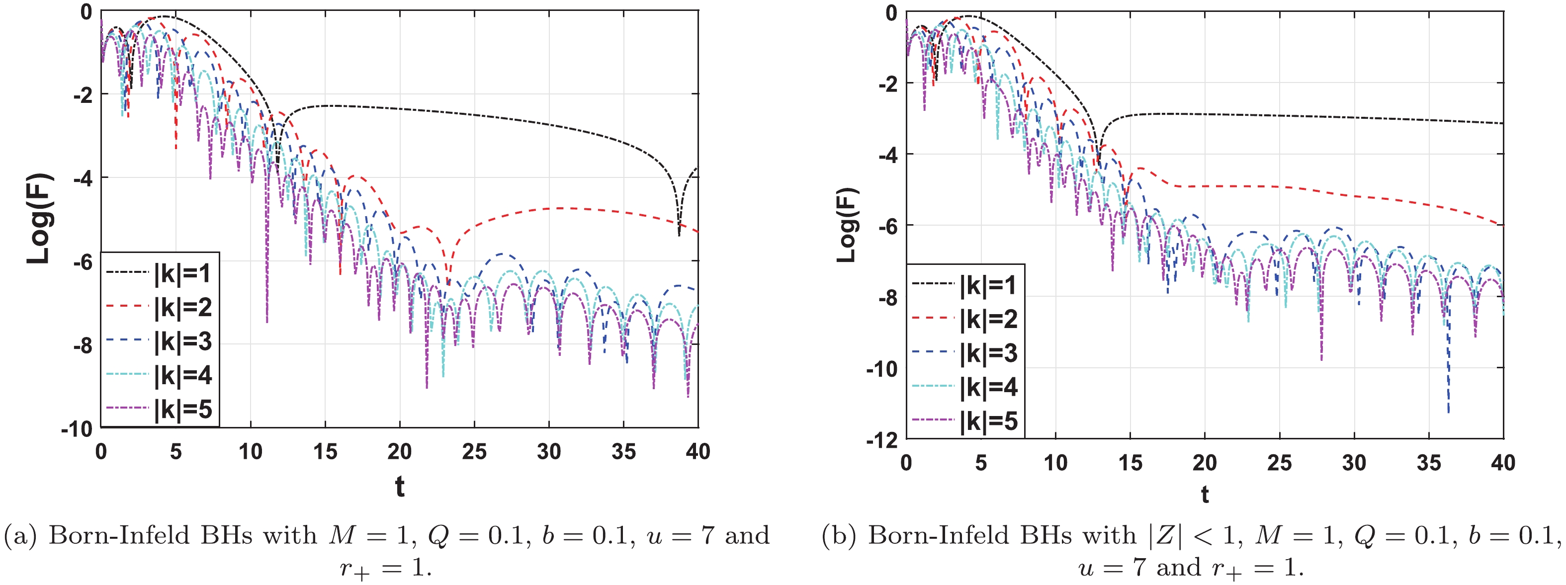
Figure 4. (color online) Dynamic evolution of Born-Infeld BHs with various
$|k|$ .Figure 3 demonstrates the evolution of the Dirac field in Born-Infeld BHs with
$ |k| = 3 $ ,$ Q = 0.1 $ , and$ n = 3, 4, 5, 6, 7, 8, 9, 10 $ . We focus on the effects of different spacetime dimensions n on Born-Infeld BHs. The absolute value of the imaginary parts of quasinormal frequencies increase as the spacetime dimension of BH increases to 10. This result shows that it takes less time for QNMs to completely decay outside the Born-Infeld BHs. In other words, it takes less time to restore equilibrium under perturbation, which indicates that it will affect the QNMs of Born-Infeld BHs with an increase in the spacetime dimension n. Furthermore, Fig. 4 shows that, for a given n,$ {\rm{Re}}(\omega) $ of the frequency increases, but$ |{\rm{Im}}(\omega)| $ of the frequency decreases with increasing$ |k| $ . Note that the oscillation frequency of QNMs is faster, but the decay is slower. -
Next, we exactly calculate the QNMs of Born-Infeld BHs in a massive Dirac field. In the massive case, the potential function
$ V(r) $ depends not only on the mass m of the Dirac field, but also on$ \omega $ . This fact makes it more complicated to utilize the WKB method to calculate the QNM frequencies. Figure 5 shows the dependence of$ V(r) $ on m for$ \omega = 1 $ . The effective potential functions are still in the form of a barrier. Figure 5 shows that the peak of the potential function$ V(r) $ increases with increasing m, where$ V(r) $ exhibits the following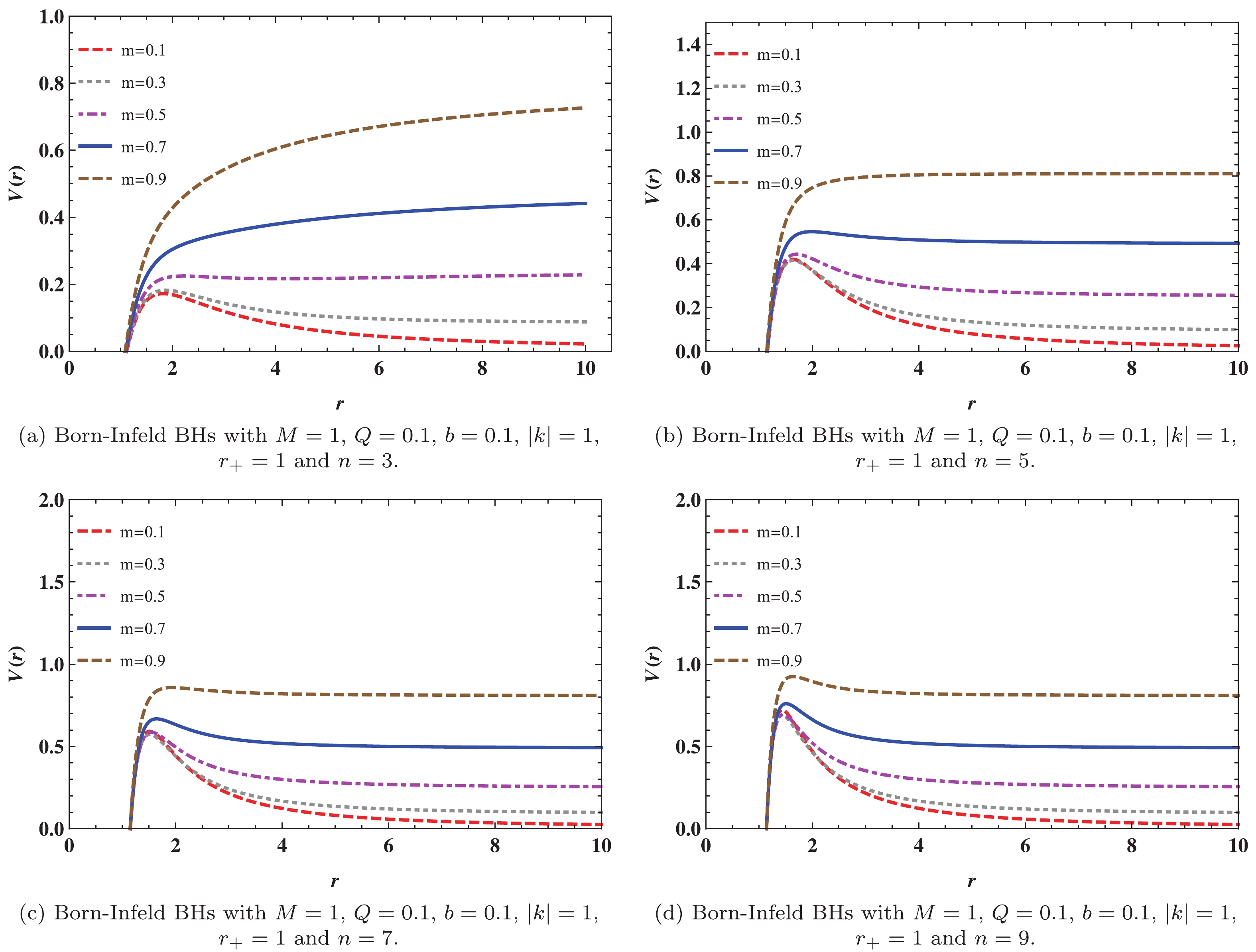
Figure 5. (color online) Behavior of Born-Infeld BH potential under massive condition.
$ V(r\rightarrow\infty) = m^{2}. $

(46) As m increases, the peak potential slowly increases. Eventually, when
$ r\rightarrow \infty $ , the summit of the peak value is less than the asymptotic value$ m^{2} $ . It is important to note that$ \omega $ is unknown at the beginning of the calculation (it is considered a typical value of$ \omega = 1 $ ) and must be self-consistently determined. Consequently, Fig. 5 can only represent the general behavior of the potential$ V(r) $ .The QNM frequency of a massive Dirac field is calculated using the WKB method. Table 5, Table 6, and Table 7 list the values of the QNM frequencies of Born-Infeld BHs for the parameter range
$ b = 0.1 $ ,$ Q = 0.1 $ . As shown in the tables, when the spacetime dimension n increases, the real and imaginary parts of the quasinormal frequency increase. In addition, the rate of oscillation$ {\rm{Re}}(\omega) $ increases, but the rate of decay$ |{\rm{Im}}(\omega)| $ decreases as$ |k| $ increases. As mass m increases,$ {\rm{Re}}(\omega) $ decreases and$ |{\rm{Im}}(\omega)| $ increases. The results show that the frequency oscillation of QNMs are slower and the decay is faster. One possible explanation is that when a disturbance occurs, the massive particles are absorbed by the BH, so the disturbance in the form of a BH carries away the energy of the gravitational wave.n $|k|=3$ 

$|k|=4$ 

$|k|=5$ 

$RN$ 

$1.1515968021-0.1943567809i$ 

$1.5419114849-0.1936812139i$ 

$1.9310725009-1.9310725009i$ 

$3$ 

$1.1515299453-0.1944290635i$ 

$1.5418153731-0.1937506829i$ 

$1.9309490124-0.1934480016i$ 

$4$ 

$1.4755292119-0.3566031472i$ 

$1.9839878478-0.3550679945i$ 

$2.4895032612-0.3543882938i$ 

$5$ 

$1.6643329773-0.4986323948i$ 

$2.2484728448-0.4962875707i$ 

$2.8275017646-0.4952509473i$ 

$6$ 

$1.7864791766-0.6259645966i$ 

$2.4264859682-0.6229378917i$ 

$3.0588107791-0.6216062186i$ 

$7$ 

$1.8678760678-0.7417338491i$ 

$2.5527693886-0.7382567926i$ 

$3.2268852313-0.7367680599i$ 

$8$ 

$1.9209447481-0.8478465144i$ 

$2.6442654611-0.8442465146i$ 

$3.3530315052-0.8428272448i$ 

$9$ 

$1.9523543509-0.9455039034i$ 

$2.7103645384-0.9421851886i$ 

$3.4491774444-0.9411518977i$ 

$10$ 

$1.9658661367-1.0354755466i$ 

$2.7659881744-1.0328956917i$ 

$3.5225784444-1.0326531373i$ 

Table 5.
$\omega$ in Born-Infeld BH ($r_{+}=1$ ,$Q=0.1$ ,$m=0.1$ ).n $|k|=3$ 

$|k|=4$ 

$|k|=5$ 

$RN$ 

$1.1501095992-0.1948497541i$ 

$1.5408771069-0.1939407203i$ 

$1.9302738954-0.1935386298i$ 

$3$ 

$1.1512527143-0.1959224385i$ 

$1.5417809717-0.1940103869i$ 

$1.9301503937-0.1936068759i$ 

$4$ 

$1.4716635239-0.3581239203i$ 

$1.9812604589-0.3558811885i$ 

$2.4873855581-0.3548924013i$ 

$5$ 

$1.6588120618-0.5010814268i$ 

$2.2445702706-0.4975913882i$ 

$2.8244741359-0.4960595044i$ 

$6$ 

$1.7797682963-0.6292545361i$ 

$2.4217307861-0.6246730881i$ 

$3.0551245677-0.6226789402i$ 

$7$ 

$1.8602668839-0.7458103989i$ 

$2.5473634088-0.7403826574i$ 

$3.2331497017-0.7348392792i$ 

$8$ 

$1.9126157415-0.8526820449i$ 

$2.6383369987-0.8467358085i$ 

$3.3484440776-0.8443502049i$ 

$9$ 

$1.9434064183-0.9510951098i$ 

$2.7039941198-0.9450201528i$ 

$3.4442573887-0.9428749815i$ 

$10$ 

$1.9563439528-1.0418450546i$ 

$2.7499171683-1.0360659718i$ 

$3.5173696678-1.0345653663i$ 

Table 6.
$\omega$ in Born-Infeld BH ($r_{+}=1$ ,$Q=0.1$ ,$m=0.2$ ).n $|k|=3$ 

$|k|=4$ 

$|k|=5$ 

$RN$ 

$1.1513234725-0.1944854686i$ 

$1.5419258726-0.1937346437i$ 

$1.9311600612-0.1934044131i$ 

$3$ 

$1.1500471235-0.1945577233i$ 

$1.5408302274-0.1938040522i$ 

$1.9300369849-0.1934724886i$ 

$4$ 

$1.4708385944-0.3583636618i$ 

$1.9809166931-0.3560005393i$ 

$2.4872077078-0.3549608303i$ 

$5$ 

$1.6564368177-0.5019917935i$ 

$2.2431563863-0.4980590023i$ 

$2.8234791729-0.4963428007i$ 

$6$ 

$1.7762398844-0.6308278393i$ 

$2.4195067261-0.6254697514i$ 

$3.0535106013-0.6231610884i$ 

$7$ 

$1.8558543032-0.7480347342i$ 

$2.5445058474-0.7414896237i$ 

$3.2205995072-0.7387415151i$ 

$8$ 

$1.9074914561-0.8555553184i$ 

$2.6349635078-0.8481391213i$ 

$3.3459534959-0.8451866092i$ 

$9$ 

$1.9376726156-0.9546224811i$ 

$2.7001810904-0.9467106038i$ 

$3.4414365679-0.9438729825i$ 

$10$ 

$1.9500505317-1.0460573872i$ 

$2.7457110128-1.0380389132i$ 

$3.5142605301-1.0357177954i$ 

Table 7.
$\omega$ in Born-Infeld BH ($r_{+}=1$ ,$Q=0.1$ ,$m=0.3$ ). -
In this work, we have calculated the QNMs of the perturbation of massless and massive Dirac fields in the background of a Born-Infeld BH. Here, the QNM frequencies are determined and tabulated using the WKB method, and the dynamic evolution of the Born-Infeld BHs is described using the finite difference method, which varies the multipole number
$ |k| $ and spacetime dimension n.The findings of this article are as follows: for massless Dirac perturbations, with a given Q, the oscillation frequency
$ {\rm{Re}}(\omega) $ increases but the decay rate$ |{\rm{Im}}(\omega)| $ decreases slowly with increasing$ |k| $ . Meanwhile, the real part of the QNM frequencies$ {\rm{Re}}(\omega) $ and the imaginary part$ |{\rm{Im}}(\omega)| $ become larger with higher dimensions.For massive Dirac perturbations of a Born-Infeld BH, the potential function
$ V(r) $ depends on the mass m and spacetime dimension n. The peak value of the potential function increases with increasing mass m. This implies that for a massive particle, the slower it oscillates, the faster it decays. The faster Born-Infeld BH oscillates in higher-dimensional spacetime, the faster it decays. The massive field particles themselves have energy, so they are absorbed by the BH when disturbed. Although the disturbance will cause the BH to take away the energy, the energy will be replenished, so with more massive field particles, the oscillation will be slower, but the decay will be faster. In higher dimensions, more of the energy of the perturbation of the BH will propagate outward, which will oscillate faster and decay faster. This is a description of the excited states of fermions (such as neutrinos) near a Born-Infeld BH.In summary, the following conclusions can be obtained: the asymptotically late time oscillation does not depend too much on the field spin and the Born-Infeld parameter. The decay is according to the oscillation, which depends more on the number of extra dimensions and the multipole number.
A natural extension of this work is to research BHs in Anti-de Sitter spacetime. The development of string theory on AdS/CFT duality, and the relationship between Born-Infeld theory and string theory, is the driving force behind this phenomenon. We therefore think it is worth understanding the various properties of BH solutions in this theory. In addition, we need to broaden our study of the high-frequency part to fully understand its physical nature. These interesting ideas will be used as follow-up research in the near future.
Dirac quasinormal modes of Born-Infeld black hole spacetimes
- Received Date: 2020-02-14
- Accepted Date: 2020-05-15
- Available Online: 2020-09-01
Abstract: Quasinormal modes (QNMs) for massless and massive Dirac perturbations of Born-Infeld black holes (BHs) in higher dimensions are investigated. Solving the corresponding master equation in accordance with hypergeometric functions and the QNMs are evaluated. We discuss the relationships between QNM frequencies and spacetime dimensions. Meanwhile, we also discuss the stability of the Born-Infeld BH by calculating the temporal evolution of the perturbation field. Both the perturbation frequencies and the decay rate increase with increasing dimension of spacetime n. This shows that the Born-Infeld BHs become more and more unstable at higher dimensions. Furthermore, the traditional finite difference method is improved, so that it can be used to calculate the massive Dirac field. We also elucidate the dynamic evolution of Born-Infeld BHs in a massive Dirac field. Because the number of extra dimensions is related to the string scale, there is a relationship between the spacetime dimension n and the properties of Born-Infeld BHs that might be advantageous for the development of extra-dimensional brane worlds and string theory.


 DownLoad: