Shadows and weak gravitational lensing by the black hole in Einstein-Maxwell-scalar theory

In general relativity (GR), black holes have so far been known as a generic result of finding exact analytical solutions to the field equations. Now the recent observations associated with gravitational waves [1, 2] and with the first image of the elliptical M87 galaxy as supermassive black hole observed by the Event Horizon Telescope (EHT) collaboration [3−5] have proven the existence of black holes in the universe. Therefore, these modern observations in connection with black holes become increasingly important to reach a deeper understanding of their attractive nature and to examine the spacetime geometry in the frame of various theories of gravity.

The Event Horizon Telescope (EHT) Collaboration [3, 4] published a black hole image in 2019: near black holes, light can be strongly deflected and even traveling in a circular path. Because of this strong deflection, as well as the fact that no light comes out of a black hole, a black hole appears as a dark disc in the sky; this disc is known as the black hole shadow. The shadow of a nonrotating black hole is a circular disc. Synge [6] conducted the first study of light deflection around a Schwarzschild black hole, and Luminet [7] simulated a shadow photograph of the black hole. In this direction, the shadow analysis was first considered around a Kaluza-Klein rotating dilaton black hole (see for example [8]). Later, the shadow analysis was extended to Einstein-Maxwell-Dilaton-Axion (EMDA) black hole and naked singularity [9]. The size and the shape of the shadow depend on the mass, the charge, and the angular momentum. We find that, for fixed values of these parameters, the shadow is slightly larger and less deformed than for its Kerr-Newman counterpart. The shadow analysis plays an important role in probing black hole spacetime geometry and accretion models in EMDA supergravity theory [10, 11]. Similarly, the null-like geodesics around compact objects can also act as the best tools to classify the spacetime structure of charged static dilaton black holes in Einstein-Maxwell-dilaton gravity [12]. Furthermore, EMDA gravity can also be regarded as an important tool in addressing the late time acceleration of the universe and thus it is worth exploring aspects of such gravity model in explaining the astrophysical observations, including shadows of M87^* and Sgr A^* black holes [13]. The rotating charged black holes with a scalar dilaton field in the environment surrounding plasma medium was also investigated with the aim of studying their shadows [14]. Also, the parametrized axially symmetric black holes can include infinite number of deformation parameters that can alter the black hole geometry, thus allowing to new methods for the shadow calculations [15]. It has then value to analyze the impact of some of these deformation parameters on the black hole shadow in order to enhance our understanding about these objects [16]. As a result of the detection of black hole shadows, many researchers have been working on theoretical modeling of black hole shadows in recent years [17−31]. It should also be noted that black hole shadows have also been extended to alternative compact object models, e.g., scalar boson and Proca stars by adapting analytical fittings of numerical solutions (see for example [32−34]).

In GR, it is well-known that a gravitational lensing has so far been described by the deflection angle of the light ray which deviates from its original path due to a distant source regarded as a massive compact object. Hence, the impact of the background spacetime on gravitational lensing has been one of the fascinating tasks in an astrophysical context. The fact to be noted here is that the first experiment pertining to testing of GR was addressed through the gravitational lensing effect (see for example [35]). The gravitational lensing has since been considered to be one of the potent tests in providing information in relation to distance sources and compact objects (e.g., black holes) and in probing their unknown aspects. An extensive analysis has been done on these lines in various situations; here we give some representatives [36−45].

To agree with the observational conclusions, it is essential to test the spacetime geometry and to study its impact on the phenomena occurring in the close vicinity of massive compact objects. In an astrophysical scenario, black holes can only possess mass M, rotation a, and electric charge Q. Of them, the black hole's rotation has been confirmed by a number of observations; see some representative references [46−51]. Reissner-Nordström (RN) black hole solution can only be characterized by mass M and charge Q [52, 53] with its interesting properties [54, 55]. One of the thought mechanisms permits black hole be charged with a positive net electric charge; see details [56, 57]. Also, the induced field can help black hole in having electric charge under the effect of magnetic field lines [58]. On these lines there have since been different solutions, including a rotating Schwinger dyon black hole solution with the electric $ Q_e $ and magnetic $ Q_m $ charges [59, 60] and regular black hole solutions associated with non-linear electrodynamics (NED) [61−68]. Here, it is worth noting that Einstein's thoery of gravity is also applicable for the low energy limit of string field theory that facilitates the dilaton scalar field. It is to be emphasized that this field involves additional term in the action with the gauge, axion and dilaton fields (see details [69, 70]). For that purpose, the heterotic string theory was also proposed using the scalar dilaton field together with the electromagnetic field [71]; here we give some representative references in connection with the dilaton fields [70−75]. Apart, in the frame of the extended theories, black hole solutions have also been considered in Refs. [76−80] and analysed with their quantum features [81−84]). Also, there exist interesting black hole solutions in EMS theory involving the dilaton field and cosmological constant [70, 85, 86]. An extensive analysis in connection with these black hole solutions in EMS theory has since been devoted to the study of their properties [86−90].

Here it must be noted that, in previous works the dilaton black hole spacetimes can be affected by the dilaton charge all through that acts as a new hair as well as a powerful tool for testing optical phenomena around the spacetime. However, in this paper we consider an interesting solution describing a charged black hole in EMS theory of gravity as the extension of RN solution involving dilaton field, as described by the line element in Eq. (1), which we can further manifest with details. This solution can directly be affected by the black hole electrical charge, thus referring to the main distinguishing characteristics from the dilaton black hole solution. It is therefore instructive to thoroughly explore remarkable aspects of such a black hole solution in EMS theory and the effects of its parameters on the optical properties around the spacetime geometry, thereby enhancing our understanding in relation to its implications in explaining astrophysical observations and in distinguishing from other black hole solutions. In this paper, we do therefore study the optical properties of this black hole solution using shadow and weak gravitational lensing with the magnification of lensed image in the strong field regime. We then analyze the influence of the EMS black hole parameters on optical phenomena, thus allowing us to gain a deeper understanding of the spacetime geometry. We intend to start investigating the shadow of the charged black hole in EMS theory using analytical calculations. Comparing analytical results to numerical simulations, which can only show the case for a specific set of parameters, analytical results illustrate exactly how impacts differ based on these parameters, as well as their general characteristics.

The paper is organized as follows. In Sec. II, we discuss the metric for a charged black hole in EMS theory of gravity, which is followed by the main study as regards the black hole shadow and the analytical solutions providing the radius of the photon sphere and the shadow. Sec. III is devoted to the study of the weak gravitational lensing with the magnification of lensed image around the black hole. We discuss our concluding remarks in Sec. IV.

Throughout the paper we use a system of units in which $ G = c = 1 $ and signature $ (-, +, +, +) $ for the metric.

Here, the action can be depicted as (see details in Refs. [70, 86])

where new quantities in the action are ϕ and $ K(\phi) $ which represent the massless scalar field and the scalar field function, respectively. It should be noted that $ K(\phi) $ is also referred to as the coupling function describing the relation between dilaton fields and the electromagnetic $ F_{\alpha\beta} $. The last term $ V(\phi) $ in the action depicts the potential pertaining to the cosmological constant Λ, thereby resulting in referring to the de-Sitter black hole solution with the dilaton field in the EMS theory; i.e. $ V(\phi) = \dfrac{\Lambda}{3} (e^{2\phi}+4+ e^{-2\phi}) $ [85]. Then the metric describing a spherically symmetric charged black hole in EMS theory in Schwarzschild coordinates (i.e., $ V(\phi) = 0 $) is then given by [86]

with radial functions $ U(r) $ and $ f(r) $ for the $ K(\phi) = \dfrac{2e^{2\phi}}{\beta e^{4\phi}+\beta-2\gamma} $ that have following forms respectively

Note that M and Q are respectively referred to as black hole's mass and electric charge, while β and γ to as dimensionless constants in EMS theory. It should be noted that $ f(r) $ and $ U(r) $ can recover the Schwarzschild and the Reissner-Nordström black hole solutions in the case of various combinations of parameter β and γ (see details in Refs. [70, 71]). It should be noted that $ f(r) $ and $ U(r) $ recovers the Schwarzschild one in case one switches off β and γ parameters. Similarly, it reduces to the Reissner-Nordström black hole in the case of $ \gamma = 0 $ and $\, \beta = 1 $. However, the above solution turns into the dilation solution in the case when $\, \beta = 0 $ and $ \gamma = -1 $ (see for example [70, 71]). The black hole horizon $ r_{h} $ can easily be determined by $ U(r) = 0 $, which is given by

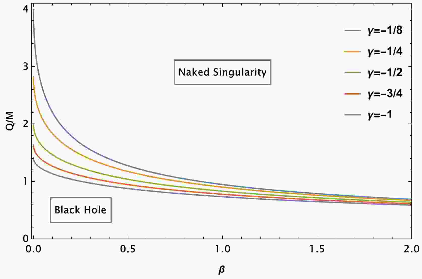
From the above equation, we note that the black hole horizon no longer exists in the case of larger parameter β, thus resulting in exhibiting the space–time as a naked singularity. We demonstrate it in Fig. 1 as the parameter space plot between the charge parameter Q and the dimensionless parameter β of the black hole for various combinations of parameter γ. As can be observed from Fig. 1, black hole sustains its existence in the region which is separated from naked singularity regions by the curves. We can also approach this issue from a different perspective, i.e., black hole extremes can be determined by imposing the following condition $ U(r) = U'(r) = 0 $ that results in obtaining the limiting values of black hole parameters as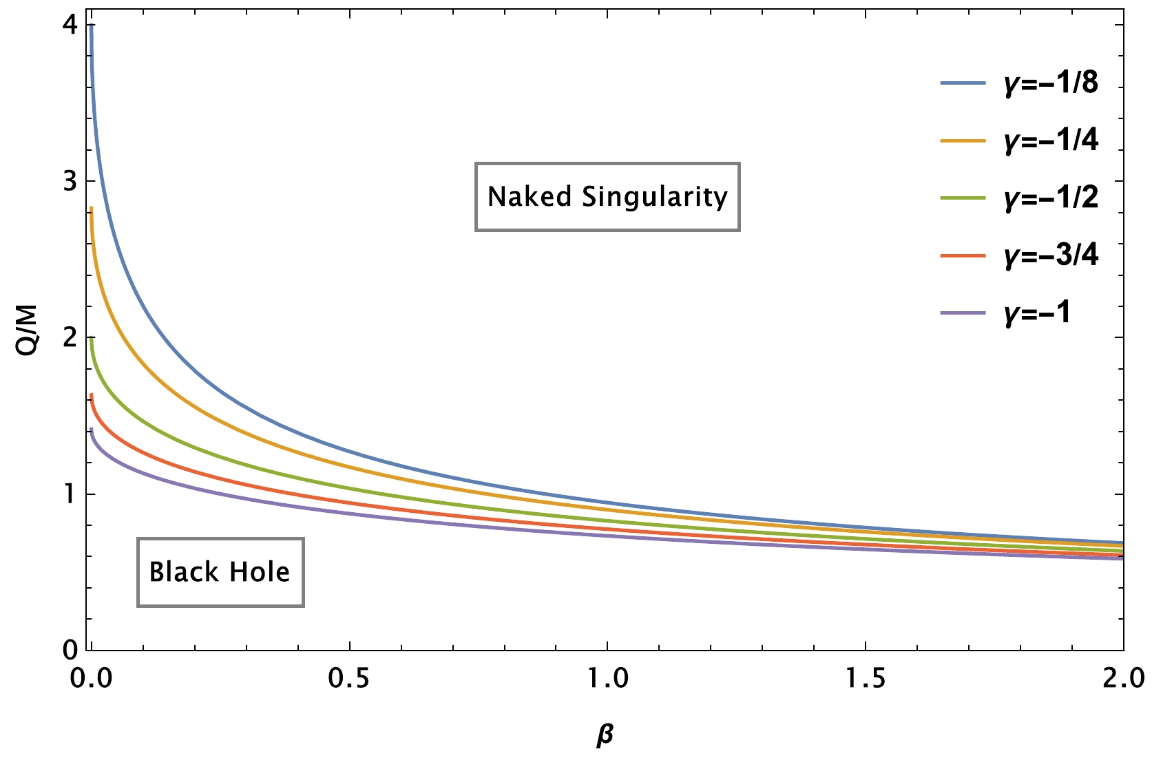

Figure 1.  (color online) Parameter space plot between the charge parameter $Q/M$ and the dimensionless parameter β of the black hole in the EMS theory for various combinations of parameter γ.

In Fig. 2 we demonstrate possible extreme values of Q as a function of γ for keeping fixed β. As can be observed from Fig. 2, extreme value of black hole charge can reach its large values as a consequence of an increase in the value of γ, while the opposite is the case for β. The extreme conditions Eqs. (4) and (5) give implicitly $ \,\beta_{\rm{max}} = 2 \gamma $ and $ {Q_{\rm{extr}}}/{M} = \sqrt{{2}/{\gamma}} $ [89] addressing the limiting values of black hole parameters.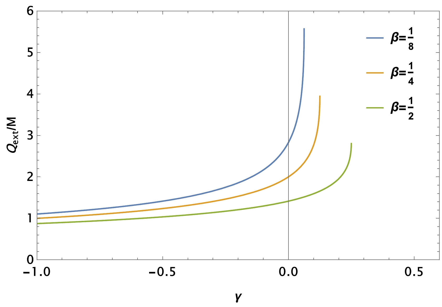

Figure 2.  (color online) Extreme values of $Q_{extr}/M$ is plotted as a function of the parameter γ for various combinations of β.

For studying shadow formation, it is necessary to consider the motion of test particles around a static and spherically symmetric black hole solution in EMS theory metric (1). The Lagrangian corresponding to the metric (1) is

To obtain the geodesic equations we use the Hamilton-Jacobi equation given as follows:

where $ {\cal{S}} $ is the Jacobi action. The following Jacobi action separable solution reads

where E and $ \ell $ are the two Killing vectors of metric (1), given by

Thus, the geodesic equations

where $ {\cal{K}} $ is the Carter separation constant and

Dimensionless quantities called impact parameters are introduced as

It depends on the critical parameters' values whether the photon is captured, scattered to infinity, or bound to orbits. Our interest is in spherical light geodesics constrained on a sphere of constant coordinate radius r with $ {\dot r} = 0 $ and $ {\ddot r} = 0 $ also known as spherical photon orbits. Without any loss of generality, we choose the equatorial plane, $ \theta = \pi/2 $. Circular orbits correspond to the maximum effective potential and the unstable photons should satisfy the following conditions:

or,

where $ r_{ps} $ is the photon sphere and marks the location of the apparent image of the photon rings and the Carter separation constant disappears by recast Eq. (13) and Eq. (14). If we consider metric (1) then we can write the radius of the photon sphere as the solution of the equation

or explicitly

The above equation is a cubic equation, hence it has three analytical roots. Using the Mathematica 11 software, the only real root is provided by

where

and

To illustrate the picture, we plot the radius of photon sphere in Fig. 3 with respect to the parameters β and γ. As can be seen from Fig. 3, the photon sphere increases as the magnitude of the γ parameter increases. However, as the parameter β increases, the photon sphere decreases first and then remains constant regardless of how much it increases. Figure 4 depicts a three-dimensional plot of the radius of the photon sphere with respect to parameters β and γ revealing their effect on $ r_{ps} $.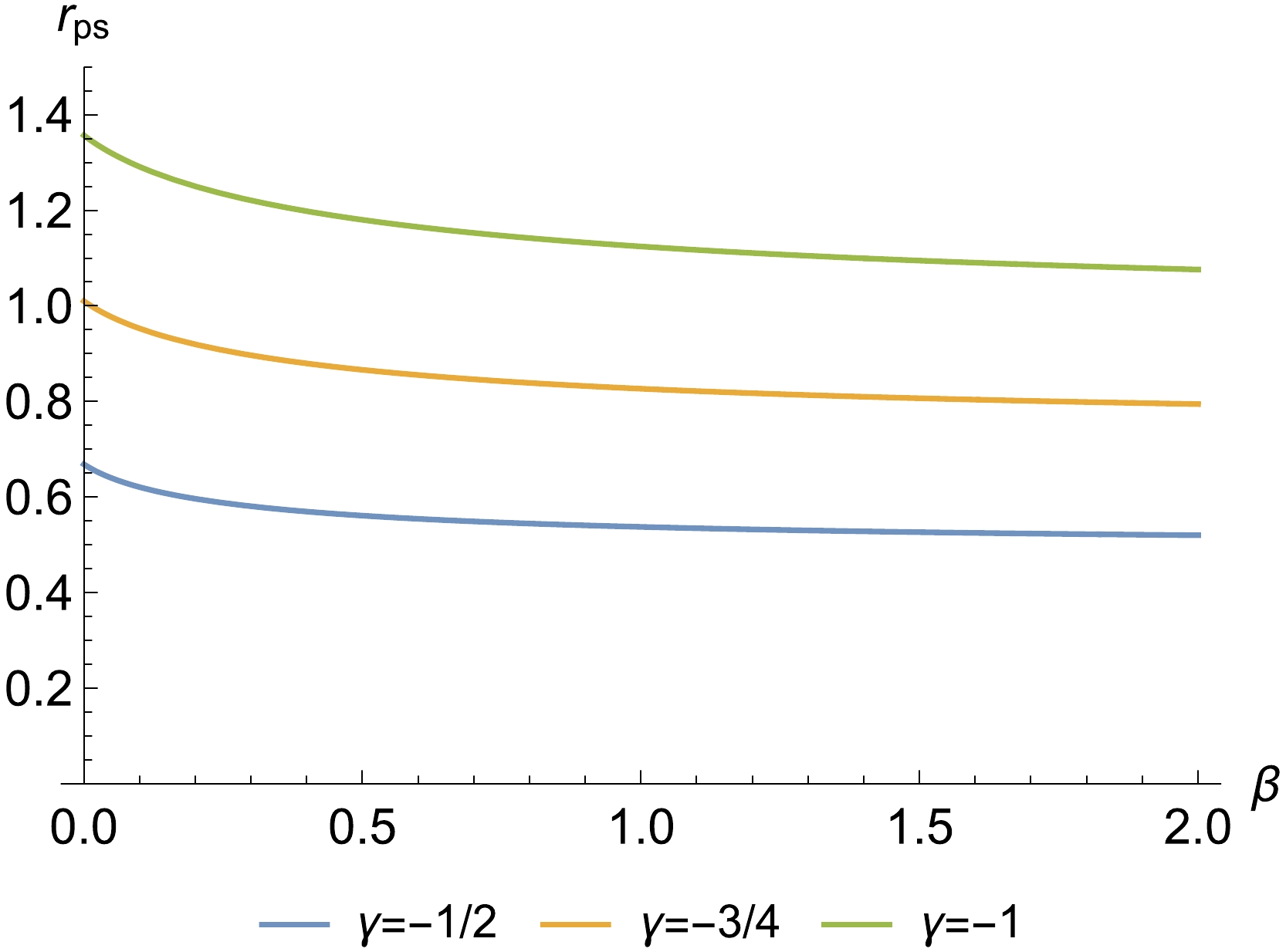

Figure 3.  (color online) Plot of Eq. (20) illustrating the dependence of $r_{ps}$ from the black hole parameters β and γ. Here $Q/M=0.66$.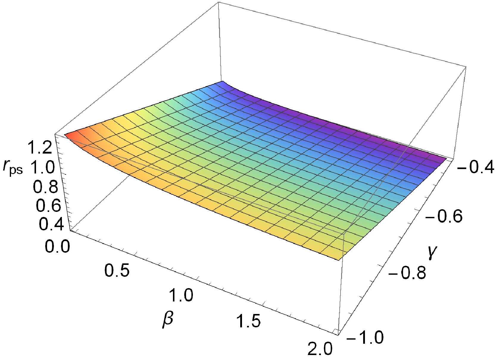

Figure 4.  (color online) Three-Dimension plot of Eq. (20) illustrating the dependence of $r_{ps}$ from the black hole parameters β and γ. Here $Q/M=0.66$.

In this view, the radius of the shadow $ R_{sh} $ is defined by the lensed image of the photon sphere

and thus it coincides in value with the impact parameter itself. Figures 5 and 6 depicts the variation of the shadow observable $ R_{sh} $ and the contours plot, respectively, for the charged black hole solution in EMS theory in the (β, γ) space to demonstrate how shadow size varies with them. We observe that an increase in the magnitude of γ parameter leads to an increase in the size of the black hole shadow. In contrast, the β parameter has the opposite effect, as it decreases the shadow of the black hole.

Figure 5.  (color online) Variation of the shadow observable $R_{sh}$ Eq. (21) for the charged black hole in EMS theory. Here $Q/M=0.66$.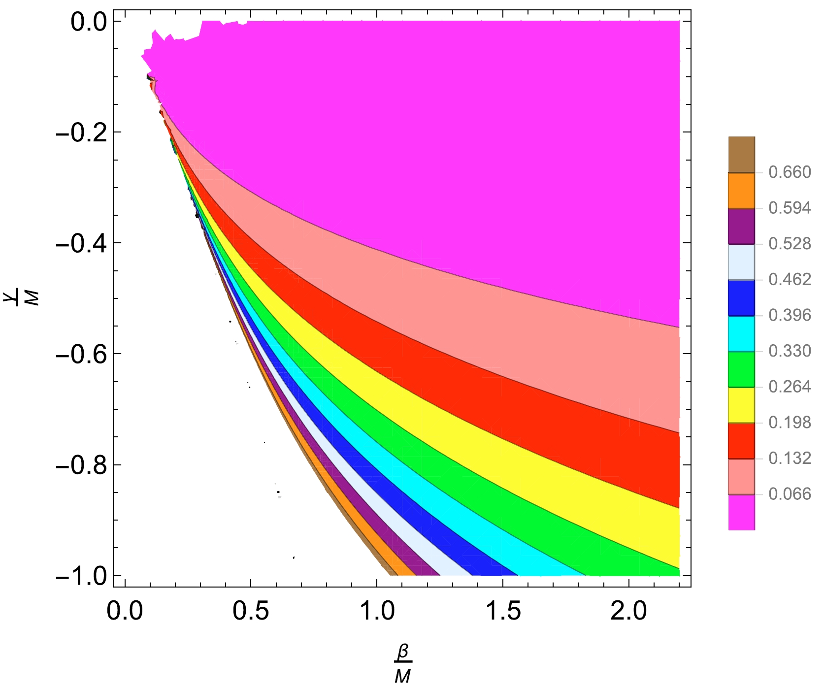

Figure 6.  (color online) Variation of the contour plot for the charged black hole in EMS theory. Here $Q/M$=0.66.

Celestial coordinates are used to describe the shadow of the black hole seen on an observer's frame [91]. Thus, we define the celestial coordinates X and Y by

where $ (r_{0},\theta_{0}) $ are the position coordinates of the observer. Assuming the observer is on the equatorial hyperplane, Eqs. (22) and (23) follow

In Table 1, we have presented the numerical values of $ r_{ps} $ and $ R_{sh} $ for a specific set of parameters. The profile of shadows cast by the charged black hole in EMS theory is shown in Fig. 7 under the influence of the parameters β and γ. Figure 7 clearly shows that the shadow radii decrease in black holes as β increases and that the decrements of the shadow radii also increase with different intervals.

	$\gamma =-1/2$			$\gamma =-3/4$			$\gamma =-1$
	$r_{ps}/M$	$R_{sh}/M$		$r_{ps}/M$	$R_{sh}/M$		$r_{ps}/M$	$R_{sh}/M$
$\beta =1$	0.5377	0.0678		0.8268	0.1433		1.124	0.24206
$\beta =3/2$	0.52669	0.05842		0.80688	0.12522		1.0949	0.21377
$\beta =2$	0.52024	0.05210		0.79469	0.11269		1.0762	0.19371

Table 1.  Numerical results for the $r_{ps}$ and $R_{sh}$ of the black hole in EMS theory. Here, $Q/M=0.66$.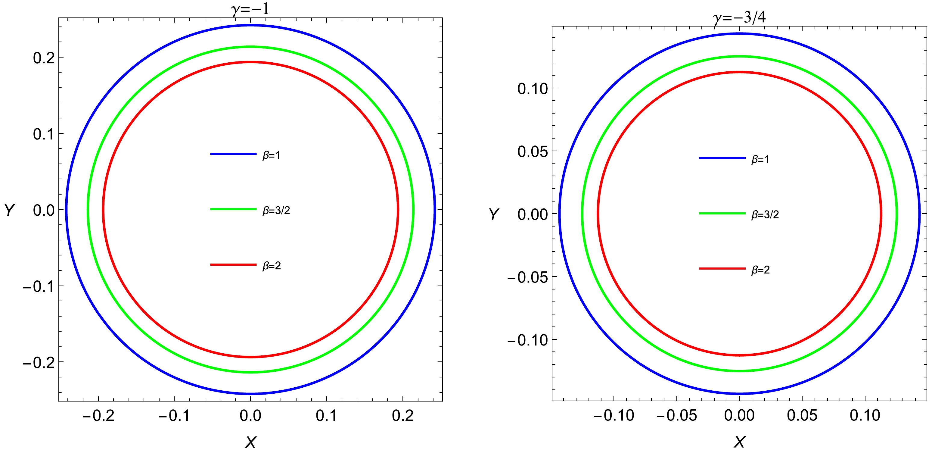

Figure 7.  (color online) The profile of shadows cast by the charged black hole in EMS theory for different values of β and γ parameters. Here, $Q/M=0.66$.

In this section, we examine the weak gravitational lensing around the black hole in the EMS theory. It is to be emphasized that the deviation of a ray of light from its original path occurs when it passes through the close vicinity of massive objects. For a weak-field approximation, the following relation can be used for metric tensor as [92]

where $ \eta_{\alpha \beta} $ and $ h_{\alpha \beta} $ refer to the expressions for Minkowski spacetime and perturbation gravity field describing EMS theory, respectively. For the weak gravitational field to be satisfied the followings for $ \eta_{\alpha \beta} $ and $ h_{\alpha \beta} $ must hold well

where $ x^{\alpha} $ refers to the spacetime coordinate.

Using the fundamental equation we can get the expression for the deflection angle around a compact object in EMS theory as follows[92].

We can write the line element Eq. 1 as follows

where $ ds^2_0 = -dt^2+dr^2+r^2(d\theta^2+\sin^2\theta d\phi^2) $. Now we can easily find components $ h_{\alpha \beta} $ of metric element in Cartesian coordinates in the form

where $ \cos^2\chi = z^2/(b^2+z^2) $ and $ r^2 = b^2+z^2 $.

Now one can define the derivatives of $ h_{00} $ and $ h_{33} $ by radial coordinate. After that, we can calculate the deflection angle $ \hat{\alpha}_b $.

With this in view, we determine explicit form of the deflection angle analytically. To this end, we restrict the location of observer to the equatorial plane, i.e., $ \theta = \pi/2 $. Afterwards, for the deflection angle to be analyzed we recall the Hamilton formalism to evaluate the geodesic equations. The standard Hamiltonian is written as

with its equations

From the Hamilton-Jacobi equation, one can also be able to write its equations as follows:

From the above equations the simplified form yields as

It should be noted that the Hamiltonian can be considered as $ H = 0 $ for the null particle, so the Eq. (32) can be rewritten on the basis of $ p_t = -E $ and $ p_{\varphi} = l $, i.e.,

so that we have the following form as

Taking $ b = {E/}{l} $, referred to as the impact parameter, into consideration we rewrite Eq. (37) as

As a matter of fact that the deviation of the light ray leads to the deflection angle by which the ray is bent from its original path when passing through a massive object. Hence, the deflection angle can be evaluated when the light is bent from its original path at the closest distance from the massive object (i.e., $ r = r_0 $). Further, to determine the impact parameter at $ r = r_0 $ one can set the following condition as

with

Taking Eqs. (39)and (40) together the impact parameter can be obtained as follows:

Following Eqs. (38) and (41) the integral form of the deflection angle by which the light is deviated from its original path can be defined by

The important point to be noted here is that one can take into account π when evaluating the deflection angle of the light ray deviating from its original trajectory if and only if the coordinate's center refers to the compact object. With this in view, the actual deflection angle by which the light is bent from its original path can be then defined by $ \hat{\alpha_b} = \bar{\alpha}-\pi $. However, it turns out to be complicated to integrate Eq. (42) analytically for the deflection angle. We therefore resort to numerical evaluation of the deflection angle $ \hat{\alpha_b} $. To gain a deeper understanding on the deflection angle of the light ray we analyse its behaviour and further show its dependence on the impact parameter for various values of black hole parameters in Fig. 8. As can be observed from Fig. 8, the deflection angle of the light ray decreases with the increase in the impact parameter $ b/M $, whereas the curves shift towards down to its smaller values with the increase in black hole charge and parameter β.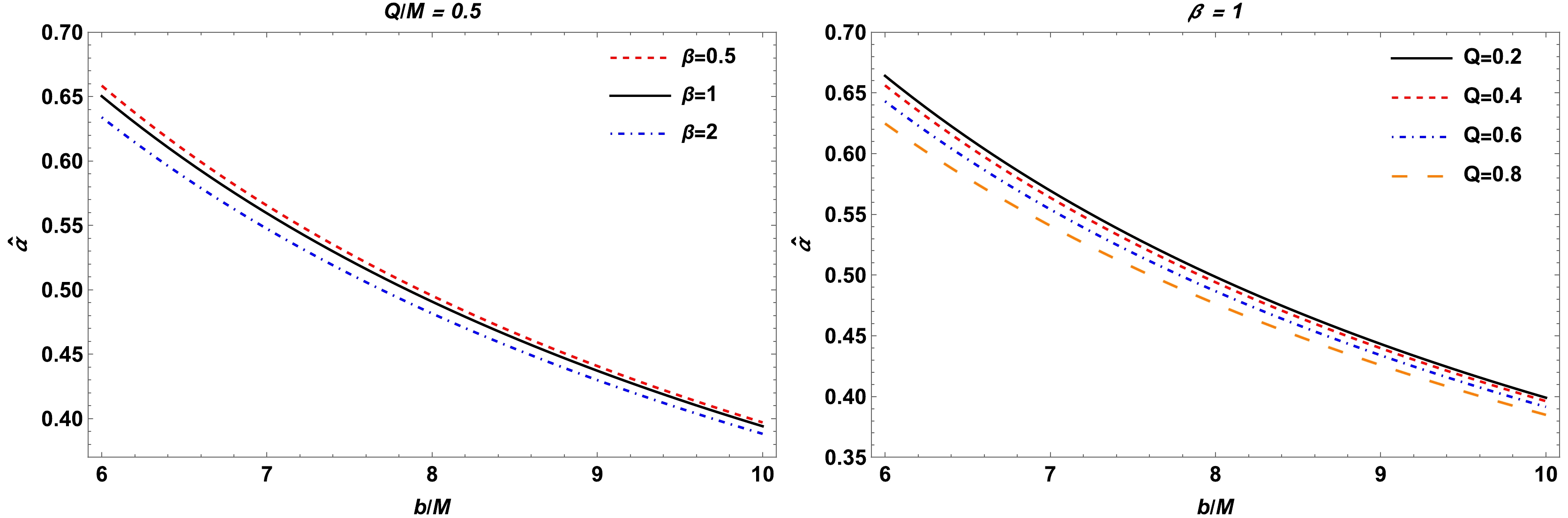

Figure 8.  (color online) Deflection angle $\hat{\alpha}$ is plotted as functions of the impact parameter b for different combinations of parameter β (left panel) and black hole charge (right panel) for the fixed γ.

Let us then examine the brightness of the image using the light's deflection angle around the black hole in EMS theory. To this end, let us write the following expression which is given in terms of the light angles, such as $ \hat{\alpha_b} $, θ and β [36, 41, 93])

Note that in the above expression we represent the following quantities, that is, the distances between the source and the observer $ D_\mathrm{s} $, the lens and the observer $ D_\mathrm{d} $ and the source and the lens $ D_\mathrm{ds} $ accordingly, whereas θ and β denote the angular position of image and source, respectively. Based on Eq. (43), the equation describing the angular position β of source is written as

Here it should be noted that we have used $ \xi(\theta) = |\hat{\alpha}_b|\,b $ with $ b = D_\mathrm{d}\theta $ [93]. With this in view, one can determine the image's shape as Einstein's ring using the radius $ R_s = D_\mathrm{d}\,\theta_E $ provided that its shape behaves like a ring. In Eq. (44) the angular part $ \theta_E $ that appears due to spacetime geometry between the source images can be given as [36]

Afterwards, we examine the magnification of brightness which is defined by (see for example [41, 94−97])

where $ I_\mathrm{tot} $ denotes the total brightness, whereas $ I_* $ stands for the unlensed brightness of the source. Raking all together the total magnification can be obtained as

Here $ x = {\beta}/{\theta_E} $ refers to a dimensionless quantity. Let us then explore the source's magnification numerically. With this aim, we analyse the dependence of the total magnification on black hole electric charge for various combinations of parameter β, and we demonstrate it in Fig. 9. As can be observed from Fig. 9, the total magnification decreases with the increase in the black hole charge, whereas its curves shift towards down to smaller values of it as a consequence of an increase in the value of parameter β.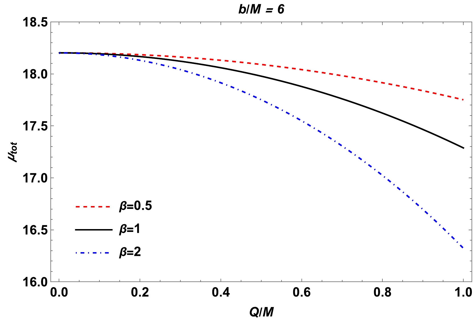

Figure 9.  (color online) Total magnification $\mu_{tot}$ is plotted as functions of black hole charge for different combinations of parameter β for the fixed γ. Note that we have set the impact parameter as $b = 6M$.

Optical studies of black holes play a crucial role for providing information in connection with distance sources, compact objects and their fascinating nature. Hence, we considered the charged black hole solution in EMS theory of gravity to understand its spacetime geometry in entirety. Also it should be emphasized that the strong field regime can have a significant impact not only on massive particle geodesics but also on the null geodesics that can give rise to a change in observable quantities including the radius of the shadow $ R_{sh} $ and etc. Therefore, it is important to study the impact of the spacetime geometry on observable quantities in the close vicinity of black hole, thus resulting in having certainty with the observational conclusions.

In this paper, we studied the optical properties, e.g., the photon motion and the weak gravitational lensing around the black hole in EMS theory for various situations. For that, we calculated the shadow cast by the black hole. We are able to obtain analytical solutions for both the radius of the photon sphere and the shadow radius. Our results show that the black hole parameters γ and β both influence the shadow of black hole. The radius of the photon sphere and the radius of the shadow both increase as the magnitude of the parameter γ increases. However, as the parameter β increases, they decrease first and then remains constant no matter how much it increases (Figs. 4 and 5). According to the obtained result, the size of the shadow (Fig. 7) of the charged black hole in EMS theory is highly dependent on the parameter β, and for large values of β, the shadow size is reduced significantly.

We also investigated the weak gravitational lensing for the black hole in EMS theory. With this regard, we calculated the deflection angle of light in the weak field regime. Further, we represented the dependence of the deflection angle on the impact parameter for different values of the black hole parameters; see Fig. 8. We inferred from the result that the value of the deflection angle gets decreased with the increase of the impact parameter, black hole charge and parameter β. Finally, we studied the total magnification of the images. The dependence of the total magnification on the black hole charge was demonstrated in Fig. 9. It is clearly seen that the total magnification gets decreased with the increase of the black hole charge and parameter β.

These obtained theoretical studies can permit to provide information in connection with black holes in EMS theory of gravity in explaining astrophysical observations.

M.A and B.A wish to acknowledge the support from Research Grant F-FA-2021-432 of the Ministry of Higher Education, Science and Innovations of the Republic of Uzbekistan.