


 Abstract
 HTML
HTML Reference
 Related
 PDF
PDF


-
Since it was established in the 1960s, the standard model (SM) of particle physics has achieved many remarkable successes and has been constantly examined for over four decades. Nowadays, the search for new physics (NP) beyond the SM is the primary endeavor in particle physics and is generally performed using two distinct techniques. On the one hand, new particles can be directly produced in high energy collisions, for instance, at the Large Hadron Collider. On the other hand, it is highly valuable to examine various low-energy observables with high precision for the indirect search for NP.
Weak decays of heavy charm and bottom quarks provide an ideal platform to test the standard model of particle physics, especially the Cabibbo-Kobayashi-Maskawa (CKM) paradigm, which describes quark mixing and CP violation. Any significant deviation of the CKM matrix from SM expectations would provide definitive clues for new physics beyond the SM. Most previous analyses have concentrated on the meson sector such as B and D mesons, while recently, heavy baryon decays have been used to determine
$ |V_{ub}/V_{cb}| $ from$ \Lambda_b \to p \mu^-\bar{\nu}_\mu $ and$ \Lambda_b \to \Lambda_c \mu^-\bar{\nu}_\mu $ [1], and$ |V_{cs}| $ from$ \Lambda_c\to \Lambda e^+\nu_e $ [2, 3].The study of the weak decays of charmed baryons
$ \Xi_c^{+,0} $ , especially$ \Xi_c\to \Xi\ell^+\nu $ decays, is highly valuable from various aspects. Firstly, the combination of form factors from lattice QCD (LQCD) and experimental results from the branching fractions of semileptonic decays allows for an independent determination of$ |V_{cs}| $ . Secondly, a comparison between theory calculations and experimental measurements provides a stringent test of theoretical models. Thirdly, compared to the isosinglet counterpart$ \Lambda_c $ , whose decays have been extensively investigated in experiments [4-12] and LQCD [13, 14], the iso-doublet$ \Xi_c^{+,0} $ baryons have more versatile decay modes. The closeness of the decay branching fractions of the exclusive$ \Lambda_c\to \Lambda \ell^+\nu $ and inclusive$ \Lambda_c \to X\ell^+\nu $ modes [8] exhibits a different pattern with heavy bottom/charm mesons. The combined analysis of the$ \Xi_c\to \Xi \ell^+\nu $ decays and$ \Lambda_c $ decays can provide a way to validate or invalidate this pattern, which is valuable for understanding the underlying dynamics in baryonic transition and testing the flavor SU(3) symmetry [15-17]. Moreover, decays of$ \Xi_c $ have played an important role in the study of the doubly-charmed baryon$ \Xi_{cc}^{++} $ [18], the precision lifetime measurement of of$ \Xi_b^0 $ [19], and the discovery of new exotic hadron candidates$ \Omega_c $ [20].Since the first observation of the inclusive semileptonic decay [21, 22], a number of different decay modes of
$ \Xi_c $ have been studied in experiments [23-27]. In addition to measuring the branching fractions of suppressed modes, the LHCb searched for CP violation in$ \Xi_c^+\to pK^-\pi^+ $ [26]. Recently, the ALICE [28] and Belle [29] collaborations measured the branching fractions for$ \Xi_c\to \Xi\ell^+\nu $ as$ {\cal{B}}_{\rm ALICE}(\Xi_{c}^0\to \Xi^- e^+\nu_{e}) = (2.43\pm0.25\pm0.35\pm0.72) {\text{%}}, $

(1) $ {\cal{B}}_{\rm Belle}(\Xi_{c}^0\to \Xi^- e^+\nu_{e}) = (1.72\pm 0.10 \pm 0.12 \pm 0.50){\text{%}} , $

(2) $ {\cal{B}}_{\rm Belle}(\Xi_{c}^0\to \Xi^- \mu^+\nu_{\mu}) = (1.71\pm 0.17 \pm 0.13 \pm 0.50){\text{%}}, $

(3) where the final errors arise from the uncertainties in
$ {\cal{B}}(\Xi_{c}^0\to \Xi^-\pi^+) $ [27].Theoretically, the
$ \Xi_{c}\to \Xi $ transition depends on six form factors that parametrize the matrix elements of vector and axial-vector currents between the$ \Xi_{c} $ and Ξ baryons. Most available theoretical analyses of these form factors are based on phenomenological models [30-35]; however, results vary substantially depending on explicit assumptions. A first-principle calculation is crucial for a precise determination of the CKM matrix element and reliable analysis of CP violation in nonleptonic decays. In this study, we use state-of-the-art LQCD techniques and, for the first time in literature, calculate the$ \Xi_{c}\to \Xi $ form factors. Predictions for semi-leptonic decay widths are also presented, based on which$ |V_{cs}| $ is extracted. Our results greatly improve upon the theoretical calculations and are more precise than the experimental measurements. These results also serve as mandatory inputs for the future analysis of non-leptonic decays, particularly in the factorization method. -
This study is based on 2+1 flavor ensembles generated using tree level tadpole improved clover fermion action and tadpole improved Symanzik gauge action. One step of Stout link smearing is applied to the gauge field used by the clover action to improve the stability of the pion mass for a given bare quark mass. The tadpole improvement factors for quarks and gluons are tuned to the fourth root of the plaquette using Stout link smearing and the original gauge links. We start from the ensemble s108 with the bare coupling
$ \beta = 10/g^2 = 6.20 $ and size$ 24^3\times 72 $ . Then, we determine the lattice spacing using Wilson flow [36] and tune the bare coupling for the s080 ensemble with a smaller lattice spacing to make their physical volumes approximately equal. Details on the two ensembles used in this paper can be found in Table 1.$\beta=10/g^2$ 

$L^3\times T$ 

a $c_{\textrm{sw}}$ 

$\kappa_l$ 

$m_{\pi} $ 

$\kappa_s$ 

$m_{\eta_s} $ 

s108 6.20 $24^3 \times 72$ 

0.108 1.161 −0.2770 285 0.1330 640 s080 6.41 $32^3 \times 96$ 

0.080 1.141 −0.2295 295 0.1318 650 Table 1. Parameters of the 2+1 flavor clover fermion ensembles used in this calculation. The
$\pi$ /$\eta_s$ masses and the lattice spacings are given in units of MeV and fm, respectively.For these two ensembles, we can use the charm quark masses
$ m_c^{s108}a = 0.485 $ and$ m_c^{s080}a = 0.235 $ , respectively, by requiring the corresponding$ J/\psi $ mass to have its physical value$ m_{J/\psi} = 3.096900(6) $ GeV [37] within 0.3% accuracy.The extraction of the
$ \Xi_c\to \Xi $ form factors requires the lattice QCD calculation of the three-point correlation function (3pt) from$ \Xi_c $ to Ξ and the two point correlation functions (2pt) of$ \Xi_c $ and Ξ. The 3pt with the weak current$ J^\mu = V^\mu-A^\mu = \bar s \gamma^\mu(1-\gamma_5)c $ is defined by$ \begin{aligned}[b] C_{3}^{V-A}(q^2, t, t_{\rm seq}) =& \int {\rm d}^3\vec x {\rm d}^3 \vec y {\rm e}^{-{\rm i}\vec p_{\Xi}\cdot \vec x} {\rm e}^{-{\rm i}\vec q\cdot \vec y} T_{\gamma'\gamma} \\ & \times \langle 0| \chi_{\gamma}^{\Xi}(\vec x, t_{\rm seq}) J^{\mu}(\vec y, t)\overline \chi_{\gamma'}^{\Xi_c}(\vec 0, 0)|0\rangle , \end{aligned} $

(4) where
$ \chi_{\gamma}^{\Xi, \Xi_c} $ is the interpolation field of Ξ and$ \Xi_c $ , respectively. T is a combination of the Dirac matrix that is chosen to project the form factor.$ C_3^{V-A}(q^2, t, t_{\rm seq}) $ is related to the bare form factor F using standard parameterization of the 3pt with one excited state:$ \begin{aligned}[b] C_3^{V-A}(q^2, t, t_{\rm seq}) =& \frac{f_{1}f_{2}m_{1}^2m_{2}^2}{4E_1E_2}{\rm e}^{-E_2(t_{\mathrm{seq}}-t)-E_1t} \\ &\times \left( F+c_1{\rm e}^{-\Delta E_1t}+c_2{\rm e}^{-\Delta E_2 (t_{\rm seq}-t)} \right), \end{aligned}$

(5) where
$ f_{i} $ ,$ m_{i} $ , and$ E_{i} $ are the decay constants, masses, and ground-state energies of$ \Xi_c $ ($ i = 1 $ ) and Ξ ($ i = 2 $ ).$ \Delta E_{i} $ describes the mass differences between the first excited states and ground states.$ c_{i} $ and the subsequent$ d_i $ are parameters for excited state contamination. For the 2pt with$ B = 1, 2 $ ,$ \begin{aligned}[b] C_{2}^{B}(t) =& \int {\rm d}^3\vec x {\rm e}^{-{\rm i} \vec p_{B} \cdot \vec x} T^{\prime}_{\gamma'\gamma} \langle 0|\chi_{\gamma}^{B}(\vec x, t) \overline \chi_{\gamma'}^{B}(\vec 0,0) |0\rangle \\ =& \frac{f_B^2m_B^2}{2E_B}{\rm e}^{-E_Bt}\left(1+d {\rm e}^{-\Delta E_B t}\right), \end{aligned}$

(6) in which
$ T^\prime $ is chosen as the identity matrix to simplify the expression. To eliminate the contributions from the excited-states, we can define the following ratios for different projection matrices T and current operators$ V^{\mu}/A^{\mu} $ :$ R_{V/A}(T,\mu) = \sqrt{\frac{C_{3}^{V/A}(q^2, t, t_{\rm seq})C_{3}^{V/A}(q^2, t_{\rm seq}-t, t_{\rm seq})} {C_2^{B_1}(t_{\rm seq}) C_2^{B_2}(t_{\rm seq}) } }, $

(7) where the subscripts V or A correspond to the vector or axial-vector current in the 3pt. After using the reduction formula, the ratios
$ R_F $ of the six form factors$ F = (f_\perp, f_+, f_0, g_\perp, g_+, g_0) $ can be constructed with different combinations of$ R_{V/A}(T, \mu) $ . Further details can be found in Appendix B. Then, we adopt the parameterization$ \begin{aligned}[b] R_F =& F\Bigg(\frac{1+c_1{\rm e}^{-\Delta E_1t}+c_2{\rm e}^{-\Delta E_2 (t_{\rm seq}-t)}}{1+d_1{\rm e}^{-\Delta E_1t_{\rm seq}}}\\&\times \frac{1+c_1{\rm e}^{-\Delta E_1 (t_{\rm seq}-t)}+c_2{\rm e}^{-\Delta E_2t}}{1+d_2{\rm e}^{-\Delta E_2t_{\rm seq}}}\Bigg)^{1/2} \\ \simeq & F[1+ c' ({\rm e}^{-\Delta E't/2}+ {\rm e}^{-\Delta E'(t_{\rm seq}-t)})], \end{aligned} $

(8) to eliminate excited-state contaminations and obtain the desired form factor F. It should be noted that Eq. (9) is the complete form of the parametrization of the 3pt and 2pt and is employed in the fit for most cases. However, for the largest negative
$ q^2 $ case$ \left(\vec{p}_2 = (0,0,2)\times\dfrac{2\pi}{La}\right) $ , the lattice results are noisy, and the contributions from the effective mass gap$ \Delta E_i $ is too small to be reliably determined from ratio fittings; thus, we will use an approximation in Eq. (10) for this case. To determine the form factor F and the parameters$ c_i $ and$ E_i $ , we fit the results of the$ R_F $ ratios with different$ t_{\mathrm{seq}} $ . In Appendix C, we also attempt to apply a joint fit for the ratio results and 2pt, which shows consistent results.The vector and axial-vector
$ c\to s $ currents on the lattice suffer from finite renormalization. Such a renormalization can be defined by the ratio of the conserved-like-vector-current$ V_{\rm c} $ and the local current V in the hadron matrix element$ \begin{aligned}[b] R^{q_1\to q_2}_V(t) =& \frac{\langle M_1(T/2)\sum_{\vec{x}}V^{q_1\to q_2}_{\rm c}(\vec{x},t)M_2(0)\rangle}{\langle M_1(T/2)\sum_{\vec{x}}V^{q_1\to q_2}(\vec{x},t)M_2(0)\rangle}\\ =& Z^{q_1\to q_2}_V+{\cal{O}}({\rm e}^{-T/4 \Delta E}), \end{aligned} $

(9) where
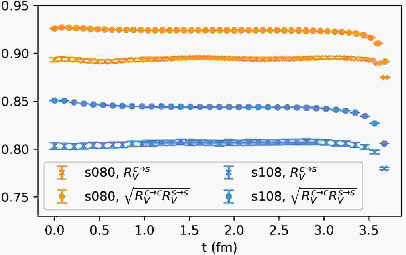
$ M_{1,2} $ are interpolating operators for pseudoscalar mesons and$ \Delta E $ is the mass gap between the ground state and first exited state. For the$ c\to s $ current, one can use either the combination$ (M_1,M_2) = (\eta_s, D_s) $ or the geometric average of those of the$ s\to s $ current and$ c \to c $ current using$ (M_1,M_2) = (\eta_s, \eta_s) $ and$ (\eta_c,\eta_c) $ , respectively. We illustrate the$ Z_V $ in Fig. 1, in which the crosses and dots correspond to$ R^{c\to s}_V(t) $ and$ \sqrt{R^{c\to c}_V(t)R^{s\to s}_V(t)} $ , respectively. Constant fits can effectively describe the data at medium large$ t\sim T/4 $ ; the difference between the two definitions decreases for the finer s080 ensemble (upper yellow data), and both definitions are closer to one compared to the values of the coarser s108 ensemble (lower blue data). Thus, the differences between the two strategies arise from discretization effects. In the following discussion, we will use$ Z^{c\to s}_V $ to obtain the central values of the final result and then repeat the analysis with$ \sqrt{Z^{c\to c}_VZ^{s\to s}_V} $ and treat the differences as the systematic uncertainties. Due to chiral symmetry breaking of the clover fermion action, the renormalization factor in the axial-vector current is not exactly equal to that of the vector. Thus, we use off-shell quark matrix elements to define$ Z_A $ as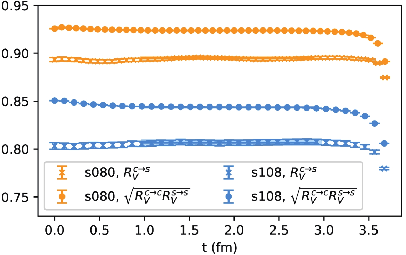
Figure 1. (color online) Lattice results for
$R_V^{c\to s}$ and$\sqrt{R_V^{c\to c}R_V^{s\to s}}$ . The bands correspond to the ground state contributions of$Z_V^{c\to s}$ and$\sqrt{Z_V^{c\to c}Z_V^{s\to s}}$ in the s080 and s108 ensembles, respectively.$ Z^{c\to s}_A\equiv Z^{c\to s}_V\sqrt{ \frac{\mathrm{Tr}[\langle c|V^{\mu}|c\rangle\gamma^{\mu}\gamma_5]}{\mathrm{Tr}[\langle c|A^{\mu}|c\rangle\gamma^{\mu}]} \frac{\mathrm{Tr}[\langle s|V^{\mu}|s\rangle\gamma^{\mu}\gamma_5]}{\mathrm{Tr}[\langle s|A^{\mu}|s\rangle\gamma^{\mu}]}}, $

(10) with the multiple off-shell quark momenta
$ p^2 $ . Using$ a^2p^2 $ extrapolation and three values of$ p^2 $ in the range of$ a^2p^2\in[4,8] $ , we obtain$ {Z_A}/{Z_V} $ = 1.010231(69) and 1.020296(68) for s108 and s080, respectively. -
By choosing different reference time slices, we perform 48
$ \times $ 393 measurements for the s108 ensemble and 72$ \times $ 436 measurements for the s080 ensemble. The lattice results of the$ R_{f_\perp} $ ratios with$ \vec{p}_{\Xi} = (0,0,1)\times \dfrac{2\pi}{La} \Bigg(\dfrac{2\pi}{La}\simeq $ $ 0.48\;{\rm GeV}\Bigg) $ are shown in Fig. 2. The$ \chi^2/d.o.f $ are less than or close to 1 for most fits of the 400 bootstrap samples, which indicates a good fit quantity. The colored bands in the left panel of Fig. 2, predicted by the fit, agree with the data points. To further validate the results, we calculate the differential summed ratio [38]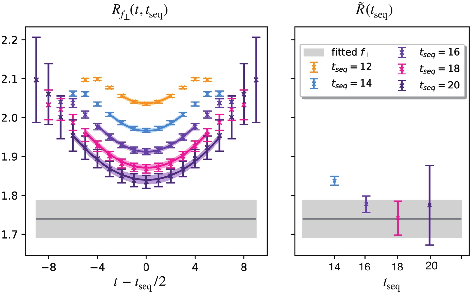
Figure 2. (color online) Lattice results for the
$f_\perp(\Xi_c\to \Xi)$ form factor in the s080 ensemble with$\vec{p}_{\Xi}=(0,0,1)\times \frac{2\pi}{La}$ in the source-sink separation range$[12a, 20a]$ . The left panel shows a two-state fit with the excited state contamination using the parametrization defined in Eq. (9), and the right panel gives the differential summed ratio. The ground-state matrix element (the grey band) obtained from the two-state fit agrees with the differential summed ratio when$t_{\rm seq}>14$ .$ \tilde{R}(t_{\rm seq}) \equiv \frac{SR(t_{\rm seq})-SR(t_{\rm seq}-\Delta t)}{\Delta t}, $

(11) and show the results in the right panel of Fig. 2, where
$ SR(t_{\rm seq})\equiv\sum_{t_c<t<t_{\rm seq}-t_c}R_F(t, t_{\rm seq}) $ ,$ t_c = 3a $ is the requirement used in the fits to suppress contributions from the higher excited states.$ \tilde{R}(t_{\rm seq}) $ agrees with the grey band from the two-state fit when$ t_{\rm seq}>14a $ .To access the
$ q^2 $ distribution, we employ the z-expansion parametrization of form factors that arises from analyticity and unitarity [39, 40]:$ f(q^2) = \frac{1}{1-q^2/(m_{\rm pole}^{f})^2} \sum\limits_{n = 0}^{n_{\rm max}} (c_{n}^f+ {d^f_{n}a^2}) [z(q^2)]^n, $

(12) where
$ z(q^2) = \frac{\sqrt{t_+-q^2} - \sqrt{t_+-t_0}}{\sqrt{t_+-q^2} + \sqrt{t_+-t_0}}. $

(13) $ t_0 = q_{\rm max}^2 = (m_{\Xi_c}-m_{\Xi})^2 $ and$ t_+ = (m_D+m_K)^2 $ , and$ d^f_{n} $ describes the discretization error of each z-expansion parameter$ c_{n}^f $ . The pole masses in the form factor are$ m_{\rm pole}^{f_+,f_\perp} = 2.112 $ GeV,$ m_{\rm pole}^{f_0} = 2.318 $ GeV,$ m_{\rm pole}^{g_+,g_\perp} = 2.460 $ GeV, and$ m_{\rm pole}^{g_0} = 1.968 $ GeV. We collect the fitted parameters in Table 2 and show the$ q^2 $ dependent form factor in the continuum limit (by eliminating the$ d^f_{n} $ terms) from the fit. The lattice results at a given$ q^2 $ are presented in Fig. 3. As shown in the figure, our form factor results for the s108 and s080 ensembles exhibit only small discretization effects.$c_0$ 

$c_1$ 

$c_2$ 

$f_{\perp}$ 

1.51±0.09 −1.88±1.21 1.71±0.49 $f_{0}$ 

0.64±0.09 −1.83±1.22 0.56±0.51 $f_+$ 

0.77±0.07 −4.09±1.18 0.35±0.49 $g_{\perp}$ 

0.56±0.07 −0.35±1.26 0.15±0.29 $g_{0}$ 

0.63±0.07 −1.37±1.36 0.15±0.29 $g_+$ 

0.56±0.08 0.00±1.38 0.14±0.29 Table 2. Results for the z-expansion parameters describing the form factors with statistical errors.
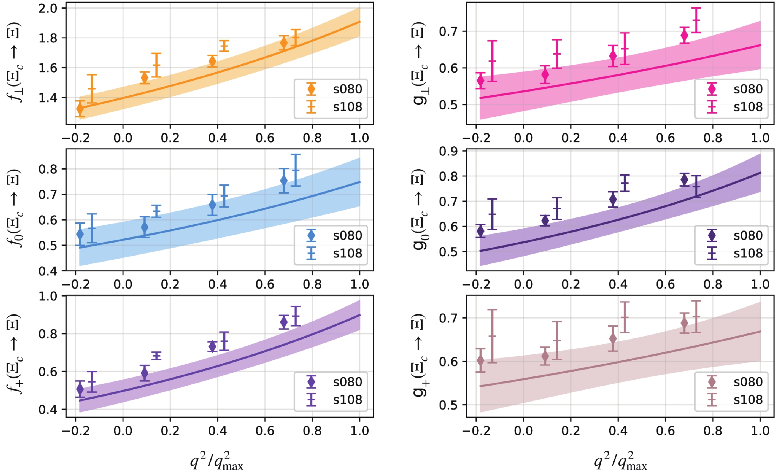
Figure 3. (color online) The
$q^2$ distribution for the$\Xi_c\to \Xi$ form factors. The z expansion approach has been used to fit the lattice data. An extrapolation to the continuum limit has been made, and the shaded regions correspond to the final results with$a\to 0$ .In Fig. 4, we use the above form factors to predict differential decay widths (in
$ {\rm ps}^{-1} {\rm GeV}^{-2} $ ) for$ \Xi_{c}^0\to \Xi^- \ell^+\nu $ divided by$ |V_{cs}|^2 $ as a function of$ q^2 $ . Results for$ \Xi_{c}^+\to \Xi^0 \ell^+\nu $ are also similar. Using the lifetime from PDG:$ \tau({\Xi^0_c}) = (1.53\pm0.06)\times 10^{-13} $ s and$ \tau({\Xi^-_c}) = (4.56\pm $ $ 0.05)\times 10^{-13} $ s, and$ |V_{cs}| = 0.97320\pm0.00011 $ [37], one can obtain the following decay branching fractions: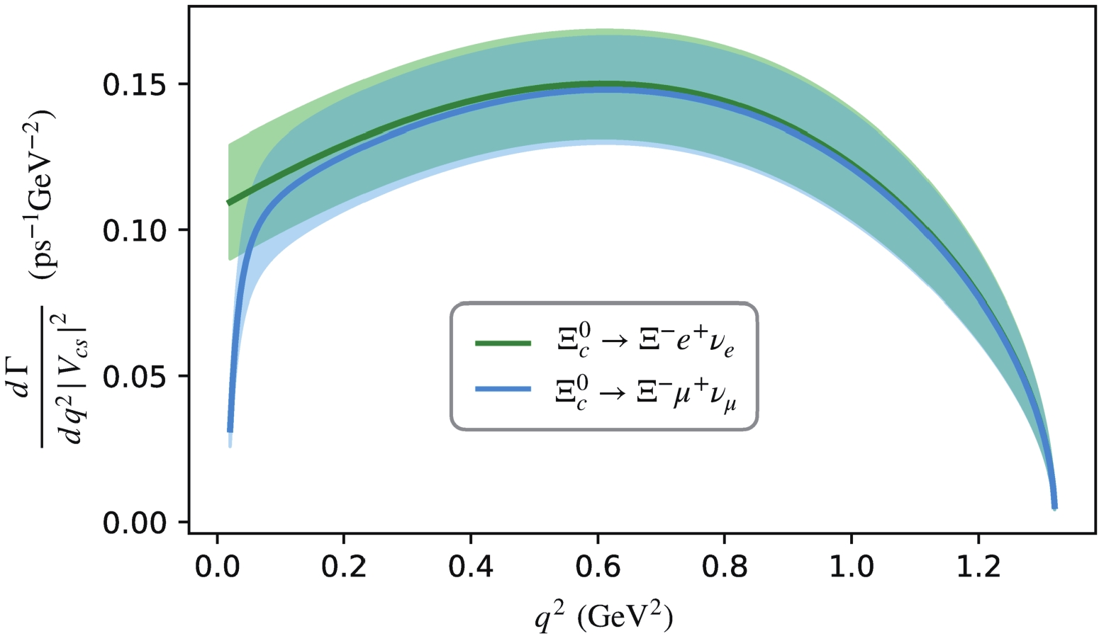
Figure 4. (color online) Predictions of the differential decay widths for
$\Xi_{c}^0\to \Xi^- e^+\nu_e$ and$\Xi_{c}^0\to \Xi^- \mu^+\nu_\mu$ , divided by$|V_{cs}|^2$ in${\rm ps}^{-1} {\rm GeV}^{-2}$ .$ \begin{aligned}[b] &{\cal{B}}(\Xi_{c}^0\to \Xi^- e^+\nu_e) = 2.38(0.30)_{\mathrm{stat.}}(0.32)_{\mathrm{ext.}}(0.07)_{\mathrm{ren.}}{\text{%}} ,\\& {\cal{B}}(\Xi_{c}^0\to \Xi^- \mu^+\nu_\mu) = 2.29(0.29)_{\mathrm{stat.}}(0.30)_{\mathrm{ext.}}(0.06)_{\mathrm{ren.}}{\text{%}},\\& {\cal{B}}(\Xi_{c}^+\to \Xi^0 e^+\nu_e) = 7.18(0.90)_{\mathrm{stat.}}(0.96)_{\mathrm{ext.}}(0.20)_{\mathrm{ren.}}{\text{%}} ,\\& {\cal{B}}(\Xi_{c}^+\to \Xi^0 \mu^+\nu_\mu) = 6.91(0.87)_{\mathrm{stat.}}(0.91)_{\mathrm{ext.}}(0.19)_{\mathrm{ren.}}{\text{%}} . \end{aligned} $

(14) The first errors arise owing to statistical fluctuations, while the second and third errors are systematic uncertainties caused by the differences between continuum-extrapolated results and those from the s080 ensemble and the differences between the results from
$ Z_{V/A}^{c\to s} $ or$ \sqrt{Z_{V/A}^{c\to c}Z_{V/A}^{s\to s}} $ in the renormalization, respectively. Our predictions for branching fractions are consistent with model results in Ref. [30]; however, they are less than those in Refs. [31, 34]. Compared to previous theoretical results, which typically have 30% ~ 50% parametric uncertainties and uncontrollable systematic uncertainties, our results have greatly improved upon the theoretical predictions. Furthermore, our calculation indicates sizable SU(3) symmetry breaking effects compared to the$ \Lambda_c\to \Lambda\ell^+\nu $ decays [3, 13].The ratio of branching fractions is predicted as
$ \begin{aligned}[b] R_{\mu/e} = &\frac{{\cal{B}}(\Xi_{c}^0 \to \Xi^- \mu^+\nu_\mu)}{{\cal{B}}(\Xi_{c}^0\to \Xi^- e^+\nu_e)} = \frac{{\cal{B}}(\Xi_{c}^+ \to \Xi^0 \mu^+\nu_\mu)}{{\cal{B}}(\Xi_{c}^+\to \Xi^0 e^+\nu_e)} \\ =& 0.962(0.003)_{\mathrm{stat.}}(0.002)_{\mathrm{syst.}}, \end{aligned} $

(15) where the majority of the uncertainties from the form factors have largely canceled. The deviation from unity arises from the mass differences between muons and electrons. This result is consistent with and more precise than the Belle measurement
$ R_{\mu/e} = 1.00\pm0.11\pm0.09 $ [29], which indicates that effects not considered by our lattice calculation are less significant at our level of precision.Our results for branching fractions are consistent with and approximately two times more precise than the measurements by the ALICE and Belle collaborations, as shown in Eqs. (1)-(3). Using the ALICE measurement [28], we obtain a theoretical constraint of
$ |V_{cs}| $ $ |V_{cs}| = 0.983(0.060)_{\mathrm{stat.}}(0.065)_{\mathrm{syst.}}(0.167)_{\mathrm{exp.}}, $

(16) where the first two uncertainties are the statistical and systematic uncertainties of the theoretical results, and the final uncertainty is dominant and arises from experimental data. Using the Belle result [29], we also have
$ |V_{cs}| = 0.834(0.051)_{\mathrm{stat.}}(0.056)_{\mathrm{syst.}}(0.127)_{\mathrm{exp.}}, $

(17) which is obtained by combining
$ \Xi_{c}^0\to \Xi^- e^+\nu_e $ and$ \Xi_{c}^0\to \Xi^- \mu^+\nu_\mu $ . Using the individual channel, we have$ |V_{cs}|_{(\ell = e)} = 0.830(0.051)_{\mathrm{stat.}}(0.055)_{\mathrm{syst.}}(0.128)_{\mathrm{exp.}} $ and$ |V_{cs}|_{(\ell = \mu)} = 0.846(0.052)_{\mathrm{stat.}}(0.056)_{\mathrm{syst.}}(0.135)_{\mathrm{exp.}} $ . Both results for$ |V_{cs}| $ from ALICE and Belle data are consistent with the global fit [37] within 1-$ \sigma $ .It is necessary to point out that the largest errors in the extracted results for
$ |V_{cs}| $ are from experimental data on$ {\cal{B}}(\Xi_c^0\to \Xi^-\pi^+) $ [27]. This can be improved by more precise measurements in the LHCb, Belle-II, BESIII, and other experiments in future. Moreover, as a conservative estimate, we have included systematic uncertainties (approximately 6%). In the continuum extrapolation, the statistical uncertainties in the two lattice ensembles are added, and the final uncertainties are also approximately 6%. -
In this study, we have generated 2+1 flavor ensembles with tree level tadpole improved clover fermion action and tadpole improved Symanzik gauge action. One step of Stout link smearing is applied to the gauge field used by the clover action. We then present the first lattice QCD calculation of the form factors governing
$ \Xi_{c}\to \Xi \ell^+\nu_{\ell} $ with two sets of newly generated ensembles. The continuum limits are taken based on calculations at two lattice spacings. Using the CKM matrix element$ |V_{cs}| $ from PDG and the$ \Xi_{c} $ lifetimes, we predict the branching fractions$\quad\quad \quad {\cal{B}}(\Xi_{c}^0\to \Xi^- e^+ \nu_{e}) = 2.38(0.30)_{\mathrm{stat.}}(0.32)_{\mathrm{syst.}} $ %,$ \quad\quad \quad{\cal{B}}(\Xi_{c}^0\to \Xi^- \mu^+ \nu_{\mu}) = 2.29(0.29)_{\mathrm{stat.}}(0.31)_{\mathrm{syst.}} $ %,$ \quad\quad \quad{\cal{B}}(\Xi_{c}^+\to \Xi^0 e^+ \nu_{e}) = 7.18(0.90)_{\mathrm{stat.}}(0.98)_{\mathrm{syst.}} $ %,$ \quad\quad \quad{\cal{B}}(\Xi_{c}^+\to \Xi^0 \mu^+ \nu_{\mu}) = 6.91(0.87)_{\mathrm{stat.}}(0.93)_{\mathrm{syst.}} $ %. Our results have greatly improved upon previous theoretical calculations and are consistent with and approximately two times more precise than measurements by the ALICE and Belle collaborations. Our calculation also indicates sizable SU(3) symmetry breaking effects compared to the$ \Lambda_c\to \Lambda\ell^+\nu $ decays. These results also serve as mandatory inputs for the analysis of non-leptonic decays in the factorization method. Using the measured branching fraction from two experiments and our lattice results, we obtain the theoretical constraint of the CKM matrix element:$ |V_{cs}| = 0.983(0.060)_{\mathrm{stat.}}(0.065)_{\mathrm{syst.}}(0.167)_{\mathrm{exp.}} $ and$ 0.834(0.051)_{\mathrm{stat.}} (0.056)_{\mathrm{syst.}} (0.127)_{\mathrm{exp.}} $ , where the errors arise from theoretical and experimental uncertainties, respectively. -
We thank Andreas Schäfer for valuable discussions, Y.B. Yin, J. Zhu, and T. Cheng for pointing out the ALICE result in Ref. [28], C.P. Shen and Y.B. Li for correspondence on the Belle measurement [29], and W. B. Qian, Y. H. Xie, H. B. Li, B. Q. Ke, and X. R. Lyu for notifying us on the studies of
$ \Xi_c $ decays in the LHCb and BESIII experiments. We greatly thank Prof. En-Ke Wang, Nu Xu and Rong-Gen Cai for their support during gauge configuration generation on the cluster, which was supported by the Southern Nuclear Science Computing Center (SNSC) and the HPC Cluster of ITP-CAS. The LQCD calculations were performed using the Chroma software suite [41] and QUDA [42-44] through the HIP programming model [45]. The numerical calculation is supported by the Priority Research Program of Chinese Academy of Sciences and performed on the CAS Xiandao-1 computing environment. The setup for the numerical simulations was conducted on the π 2.0 cluster supported by the Center for High Performance Computing at Shanghai Jiao Tong University. -
While lattice QCD is an ab-initio approach that can handle strong interactions in hadron physics, the precision in the calculation is highly limited to various systematic uncertainties. A major systematic uncertainty resides in the ensembles. In this study, we generated two sets of 2+1 flavors clover fermion ensembles with lattice spacings
$ a = 0.108 $ and$ 0.08 $ fm. The sea quark masses are demarcated by pseudoscalar mesons ($ \pi $ for the light quark pair$ \bar{q}q $ and$ \eta_s $ for the$ \bar{s}s $ case). For example, the left panel of Fig. A1 illustrates the determination of pion mass through the two-point function in s108 and s080, respectively. The fit results are given as$ m_{\pi}^{s108} = $ $ 284.5(1.5) $ MeV with$ \chi^2/d.o.f = 0.80 $ and$ m_{\pi}^{s080} = $ $ 295.0(8) $ MeV with$ \chi^2/d.o.f = 0.82 $ . For the case of charmed baryons, it is reasonable to assume that the contributions of the sea charm and heavier quarks are neglected. The valence charm quark mass is determined by tuning the$ J/\psi $ mass, as shown in the right panel of Fig. A1, where the disconnected diagrams are not considered. The fitted results are$ m_{J/\psi}^{s108} = 3.09657(32) $ GeV and$ m_{J/\psi}^{s080} = $ $ 3.08979(31) $ GeV, respectively, which are consistent with the physical$ J/\psi $ mass within 0.3% accuracy.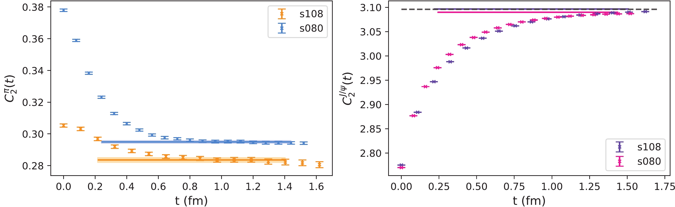
Figure A1. (color online) Effective mass plots compared with 2-state fitted plateaus for pions (left panel) and
$J/\psi$ (right panel) in different ensembles, in which the t-range of fitted plateaus indicate the range of data selected for the fit, and the dashed line in right panel denotes the physical$J/\psi$ mass. -
As in Eq. (5), the projected ratios of correlation functions can be defined as
$\tag{B1} \begin{aligned}[b]& R_1\equiv \frac{R_V(I, z)+R_V(\gamma^0, z)}{2}, \\& R_2\equiv R_V(\gamma^z, 0), \\& R_3\equiv R_V(\gamma_5\gamma^x, y), \\& R_4\equiv \frac{R_A(\gamma_5, z)+R_A(\gamma_5\gamma^0, z)}{2}, \; \\& R_5\equiv R_A(\gamma_5\gamma^z, 0), \\& R_6\equiv R_A(\gamma^x, y). \end{aligned} $

We can construct the combined ratio
$ R_F $ of the six form factors$ F = (f_\perp, f_+, f_0, g_\perp, g_+, g_0) $ as$ R_{f_\perp} = \frac{R_3}{4m_1N_{z}\hat{p}}, $

$\tag{B2} R_{g_\perp} = \frac{R_6}{4m_1N_{z}\hat{p}}, $

$\tag{B3} \begin{aligned}[b] R_{f_0} =& -\frac{\left(E_{2}-m_{1}\right)\left(m_{1}^{2}-m_{2}^{2}\right)+\left(E_{2}+m_{1}\right) q^{2}}{8 m_{1}^{2}\left(m_{1}-m_{2}\right)\left(E_{2}+m_{2}\right) N_{z} \hat{p}} R_{1} \\ & +\frac{m_{1}^{2}-m_{2}^{2}+q^{2}}{8 m_{1}^{2}\left(m_{1}-m_{2}\right) N_{z} \hat{p}} R_{2} \\&+\frac{2 m_{1} E_{2}-m_{1}^{2}-m_{2}^{2}+q^{2}}{8 m_{1}^{2}\left(m_{2}+E_{2}\right) N_{z} \hat{p}} R_{3}, \end{aligned} $

$\tag{B4}\begin{aligned}[b] R_{f_+} =& -\frac{\left(E_{2}-m_{1}\right)\left[\left(m_{1}+m_{2}\right)^{2}-q^{2}\right]}{8 m_{1}^{2}\left(E_{2}+m_{2}\right)\left(m_{1}+m_{2}\right) N_{z} \hat{p}} R_{1} \\ & +\frac{\left(m_{1}+m_{2}\right)^{2}-q^{2}}{8 m_{1}^{2}\left(m_{1}+m_{2}\right) N_{z} \hat{p}} R_{2} \\&+\frac{2 m_{1} E_{2}-m_{1}^{2}-m_{2}^{2}+q^{2}}{8 m_{1}^{2}\left(m_{2}+E_{2}\right) N_{z} \hat{p}} R_{3}, \end{aligned}$

$\tag{B5} \begin{aligned}[b]R_{g_0} = & \frac{\left(E_{2}+m_{1}\right)\left(m_{1}^{2}-m_{2}^{2}\right)+\left(E_{2}-m_{1}\right) q^{2}}{8 m_{1}^{2}\left(m_{1}+m_{2}\right)\left(E_{2}-m_{2}\right) N_{z} \hat{p}} R_{4} \\& -\frac{m_{1}^{2}-m_{2}^{2}+q^{2}}{8 m_{1}^{2}\left(m_{1}+m_{2}\right) N_{z} \hat{p}} R_{5} \\ & + \Bigg[\frac{2 m_{1}\left(E_{2}-m_{2}\right)-m_{1}^{2}+m_{2}^{2}}{8 m_{1}^{2}\left(E_{2}-m_{2}\right) N_{z} \hat{p}} \\&+\frac{\left(m_{1}-m_{2}\right) q^{2}}{8 m_{1}^{2}\left(E_{2}-m_{2}\right)\left(m_{1}+m_{2}\right) N_{z} \hat{p}} \Bigg] R_{6}, \end{aligned} $

$ \begin{aligned}[b]R_{g_+} = & \frac{\left(E_{2}+m_{1}\right)\left[\left(m_{1}-m_{2}\right)^{2}-q^{2}\right]}{8 m_{1}^{2}\left(E_{2}-m_{2}\right)\left(m_{1}-m_{2}\right) N_{z} \hat{p}} R_{4} \\ & -\frac{\left(m_{1}-m_{2}\right)^{2}-q^{2}}{8 m_{1}^{2}\left(m_{1}-m_{2}\right) N_{z} \hat{p}} R_{5} \\ & + \Bigg[\frac{2 m_{1}\left(E_{2}-m_{2}\right)-m_{1}^{2}+m_{2}^{2}}{8 m_{1}^{2}\left(E_{2}-m_{2}\right) N_{z} \hat{p}} \end{aligned} $

$\tag{B6} \begin{aligned}[b]&+\frac{\left(m_{1}+m_{2}\right) q^{2}}{8 m_{1}^{2}\left(m_{1}-m_{2}\right)\left(E_{2}-m_{2}\right) N_{z} \hat{p}} \Bigg] R_6, \end{aligned} $

where
$ m_1 $ is the mass of$ \Xi_c $ ;$ m_2,\; E_2 $ are the mass and energy of Ξ, respectively;$ \hat{p} = {2\pi}/{La}\simeq0.48 $ GeV is the unit momentum for both s108 and s080; and$ \vec{p}_{\Xi} = $ $ (N_x, N_y, N_z)\times\hat{p} $ . -
Here, we compare the fit results of the form factors
$ f_{\perp} $ from the ratios$ R_{f_{\perp}} $ with different$ t_{\mathrm{seq}} $ as well as from a joint fit that applies to the ratios and 2pt. Fig. C1 shows the comparison of the fitted results with different strategies. Compared with the first fit strategy in Fig. C1(a), the joint fit in the right panel produces consistent fit result with a smaller error and hence gives a stronger constraint of$ \Delta E_i $ than the ratios from the joint fit. For a conservative estimate, we adopt the first fit strategy in the main text.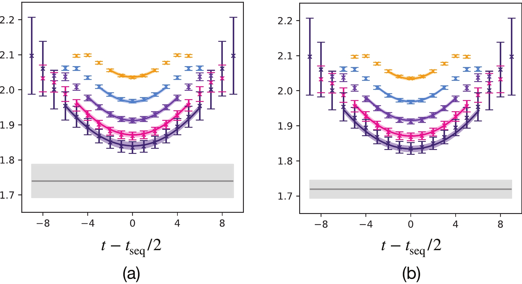
Figure C1. (color online) A comparison of the fit results of
$f_\perp$ from the ratio$R_{f_{\perp}}(t,t_{\mathrm{seq}})$ with Eq. (9) (a) and from a joint fit with the ratio$R_{f_{\perp}}(t,t_{\mathrm{seq}})$ as well as the 2pt$C_2^{(1,2)}(t)$ (b) in the s080 ensemble with$\vec{p}_{\Xi}=(0,0,1)\times \dfrac{2\pi}{La}$ .
First lattice QCD calculation of semileptonic decays of charmed-strange baryons Ξc
- Received Date: 2021-05-06
- Available Online: 2022-01-15
Abstract: While the standard model is the most successful theory to describe all the interactions and constituents of elementary particle physics, it has been constantly scrutinized for over four decades. Weak decays of charm quarks can be used to measure the coupling strength between quarks in different families and serve as an ideal probe for CP violation. As the lowest charm-strange baryons with three different flavors,


 DownLoad: