


 Abstract
 HTML
HTML Reference
 Related
 PDF
PDF


-
The
$ B_{c} $ meson stands out due to its composition of two heavy quarks, making it a unique flavor-asymmetric heavy meson. It was initially observed by the CDF collaboration in 1998 [1]. In the context of the Standard Model (SM), this meson possesses definite b and c quantum numbers and lies below the threshold for$ BD $ meson formation [2]. Consequently, it remains stable against strong and electromagnetic interactions, undergoing only weak decay processes [3]. The weak decay of the$ B_{c} $ meson is typically categorized into three types, owing to the comparable contributions from the b and c quarks: (1) b quark decay with the c quark as a spectator; (2) c quark decay with b quark as a spectator; and (3) annihilation of both the b and c quarks, which contributes less significantly. Estimates suggest that approximately 70% of the total decay rate arises from c-quark decays, while b-quark decays and annihilation contribute 20% and 10%, respectively [4]. The diverse range of weak decay channels offered by the$ B_{c} $ meson presents an opportunity to test the Standard Model and search for potential signals of new physics [5].Currently, various methodologies are employed to investigate the weak decay of the
$ B_{c} $ meson, including QCD factorization (QCDF) [6−8], perturbative QCD (PQCD) [9, 10], and soft-collinear effective theory (SCET) [11]. The QCD factorization approach is initially employed in the research of two-body non-leptonic decays of B mesons. It is feasible to consider taking the b quark mass to infinity and neglecting higher-order contributions of$ 1/m_b $ within the framework of QCDF. The amplitude of two-body non-leptonic decays can be expressed as the product of the form factor describing the transition from the initial state meson to the final state meson and the light-cone distribution amplitude of the final meson in the heavy quark limit. Recently, QCDF has been extended to encompass the three-body decay processes of B mesons [12]. Soft-Collinear Effective Theory (SCET) originates from the methodology for computing hadronic matrix elements based on collinear factorization. SCET is a framework describing the interactions between high-energy quarks, collinear gluons, and soft gluons. It has been extensively applied to calculate the decays of B mesons (quark-antiquark bound states involving bottom quarks), properties of hadronic jets produced in particle collisions during the generation of quarks or gluons, and electroweak interactions of the Higgs boson. SCET not only exhibits the ability to handle multiple soft energy scales but also provides a systematic power-counting scheme. The PQCD approach effectively curbs non-perturbative effects through the introduction of transverse momentum ($ K_T $ ) and Sudakov factors. Non-perturbative contributions are embedded within the hadron wave functions, and their parameters are to be determined experimentally. Consequently, the PQCD approach has found extensive application in the analysis of two-body B meson decays. This approach is capable of dealing with the contributions of both factorizable and non-factorizable annihilation diagrams in a comprehensive and systematic manner, demonstrating wide applicability and computational feasibility. For the decay processes of$ B_{c} $ mesons involving non-relativistic heavy quarks, particularly when the charm quark in the final-state D meson is approximately collinear, the PQCD method based on$ K_T $ factorization offers an effective solution. This method not only computes various Feynman diagrams but also exhibits excellent performance in handling non-factorizable and annihilation diagrams. The successful application of the PQCD method in predicting decays such as$ B\to J/\psi D $ [13] and$ B^0\to D_{s}^{-}K^{+} $ [14] further validates its efficacy and reliability.The complexity involved in studying the decays of three-body hadronic B mesons is universally recognized as being significantly greater than that of two-body decays. Fortunately, it has been observed that a majority of these decays are predominantly governed by low-energy scalar, vector, and tensor resonance states, which can be effectively described within the framework of quasi-two-body decay [15, 16]. CP violation is a captivating phenomenon in the realm of particle physics. The SM provides a comprehensive framework for elucidating CP violation; however, certain unexplained phenomena persist [17]. Currently, one avenue for investigating CP violation entails exploring the CKM matrix and hadronic matrix elements, while another involves scrutinizing interference arising from different particle types.
We introduce the
$ \rho^{0}-\omega-\phi $ mixing mechanism to compute the branching ratios and CP violation in the quasi-two-body approach. Positive and negative electrons annihilate into photons, which then polarize the vacuum to form the$ \phi (1020) $ ,$ \rho^0(770) $ , and$ \omega(782) $ mesons. These mesons can then decay into$ \pi^+\pi^- $ or$ K^{+} K^{-} $ pairs. Meanwhile, the momentum can also be transferred through the VMD model [18, 19]. Since the intermediate-state particle is an unphysical state, we need convert it from an isospin field into a physical field from an isospin field through the matrix R [20]. Then, we can obtain the physical states of$ \rho^{0} $ , ω, and ϕ. It is worth noting that there is no$ \rho^{0}-\omega-\phi $ mixing in the physical states, and we neglect the contribution of higher-order terms [21]. The physical states$ \rho^{0}-\omega-\phi $ can be expressed as linear combinations of the isospin states$ \rho^{0}_{I}-\omega_{I}-\phi_{I} $ . The transformation between the physical and isospin fields in the intermediate state of the decay process is described by the matrices R. The off-diagonal elements of R contain information about$ \rho^{0}-\omega-\phi $ mixing. Based on the isospin representation of$ \phi_{I} $ ,$ \rho_{I} $ , and$ \omega_{I} $ , the isospin vector$ |I,I_{3}> $ can be constructed, where$ I_3 $ denotes the third component of isospin. Currently, the Large Hadron Collider (LHC) possesses high energy and high luminosity and is capable of collecting approximately$ 10^9 $ $ B_{c} $ meson events annually [22]. We anticipate that our prediction can be validated through the following experiments at LHC experiment.This paper is structured as follows: In Sec. II, we investigate CP violation in the decay process
$ B_c^+ \rightarrow D_{(s)}^+ \pi^+ \pi^- $ via a mixing mechanism involving three vector mesons. In Sec. III, we extend this analysis to the decay process$ B_c^+ \rightarrow D_{(s)}^+ K^+ K^- $ . In Sec. IV, we derive an integral form representation of local CP violation. In Sec. V, we introduce a formalism for localized CP violation and provide a comparative analysis of the data. In Sec. VI, we examine the branching ratios of$ B_c^+ \rightarrow D_{(s)}^+ \pi^+ \pi^- $ and$ B_c^+ \rightarrow D_{(s)}^+ K^+ K^- $ . Finally, we present a comprehensive summary and conclusion. -
We present decay diagrams of the
$ B_{c}^{+} \rightarrow D_{(s)}^{+}\rho^{0} $ (ω, ϕ)$ \rightarrow D_{(s)}^{+}\pi^{+}\pi^{-} $ process in Fig. 1, aiming to provide a more comprehensive understanding of the mixing mechanism. The quasi-two-body approach used in this study is clearly illustrated in Fig. 1. In these decay diagrams, the processes depicted in Fig. 1(a) represent direct decay modes, where$ \pi^{+}\pi^{-} $ pairs are produced via the$ \rho^0 $ meson. Compared to the direct decay processes depicted in Fig. 1(a), the$ \pi^{+}\pi^{-} $ pair can also be generated through a distinct mixing mechanism. Fig. 1(b) and 1(c) indicate that the ϕ and ω mesons undergo resonant decay to a$ \pi^{+}\pi^{-} $ meson pair through the mixture with the$ \rho^0 $ meson. The black dots in the figure represent the resonance effect between these two mesons, denoted by the mixing parameter$ \Pi_{V_{i} V_{j}} $ . Although the contribution from this mixing mechanism is relatively small compared to that of Fig. 1(a), it is considered in our calculations. Given that the branching ratio of$ \rho^0 \rightarrow \pi^{+} \pi^{-} $ is approximately$ 100$ %, we can neglect the direct contributions from$ \phi \rightarrow \pi^{+} \pi^{-} $ and$ \omega \rightarrow \pi^{+} \pi^{-} $ . Consequently, since the direct decays of$ \phi \rightarrow \pi^{+} \pi^{-} $ and$ \omega \rightarrow \pi^{+} \pi^{-} $ are negligible, the even smaller contribution from resonant mixing can also be disregarded.
Figure 1. Decay diagrams of
$\ B_{c}^{+} \rightarrow D_{(s)}^{+}\rho^{0}$ (ω,ϕ)$ \rightarrow D_{(s)}^{+}\pi^{+}\pi^{-}$ process.The amplitude of the
$ B_{c}^{+} \rightarrow D_{(s)}^{+}\rho^{0} $ (ω, ϕ)$ \rightarrow D_{(s)}^{+}\pi^{+}\pi^{-} $ decay channel can be described as follows:$ A = \left \langle D_{(s)}^+\pi^+\pi^-\left | H^{T} \right | \ B_{c}^+ \right \rangle +\left \langle D_{(s)}^+\pi^+\pi^-\left | H^{P} \right | B_{c}^+ \right \rangle, $

(1) where
$ \left \langle D_{(s)}^{+}\pi^{+}\pi^{-}\left | H^{P} \right | \ B_{c}^{+} \right \rangle $ and$ \left \langle D_{(s)}^{+}\pi^{+}\pi^{-}\left | H^{T} \right | \ B_{c}^{+} \right \rangle $ represent the amplitudes associated with penguin-level and tree-level contributions, respectively. Neglecting higher-order terms, the amplitudes are as follows:$ \begin{split} &\left \langle D_{(s)}^+\pi^+\pi^-\left | H^{T} \right | \ B_{c}^+ \right \rangle \\ =\;& \frac{g_{\rho^0 \rightarrow \pi^+ \pi^-}}{({s-m_{\rho ^0}^{2}+{\rm i}m_{\rho ^0} \varGamma _{\rho ^0}})}t_{\rho} \\ &+\frac{g_{\rho^0 \rightarrow \pi^+ \pi^-}}{({s-m_{\rho ^0}^{2}+{\rm i}m_{\rho ^0} \varGamma _{\rho ^0}})({s-m_{\omega}^{2}+{\rm i}m_{\omega} \varGamma_{\omega}})}\widetilde{\Pi}_{\rho\omega}t_{\omega} \\ &+\frac{g_{\rho^0 \rightarrow \pi^+ \pi^-}}{({s-m_{\rho ^0}^{2}+{\rm i}m_{\rho ^0} \varGamma _{\rho ^0}})({s-m_{\phi}^{2}+{\rm i}m_{\phi} \varGamma_{\phi}})}\widetilde{\Pi}_{\rho\phi}t_{\phi}, \end{split} $

(2) $ \begin{split} &\left \langle D_{(s)}^+\pi^+\pi^-\left | H^{P} \right | \ B_{c}^+ \right \rangle \\ =\;& \frac{g_{\rho^0 \rightarrow \pi^+ \pi^-}}{({s-m_{\rho ^0}^{2}+{\rm i}m_{\rho ^0} \varGamma _{\rho ^0}})}p_{\rho}\\ &+\frac{g_{\rho^0 \rightarrow \pi^+ \pi^-}}{({s-m_{\rho ^0}^{2}+{\rm i}m_{\rho ^0} \varGamma _{\rho ^0}})({s-m_{\omega}^{2}+{\rm i}m_{\omega} \varGamma_{\omega}})}\widetilde{\Pi}_{\rho\omega}p_{\omega} \\ & +\frac{g_{\rho^0 \rightarrow \pi^+ \pi^-}}{({s-m_{\rho ^0}^{2}+{\rm i}m_{\rho ^0} \varGamma _{\rho ^0}})({s-m_{\phi}^{2}+{\rm i}m_{\phi} \varGamma_{\phi}})}\widetilde{\Pi}_{\rho\phi}p_{\phi}, \end{split} $

(3) where the tree-level (penguin-level) amplitudes
$ t_{\rho}\left(p_{\rho}\right) $ ,$ t_{\omega}\left(p_{\omega}\right) $ , and$ t_{\phi}\left(p_{\phi}\right) $ correspond to the decay processes$ B_{c}^{+} \rightarrow D_{(s)}^{+}\rho^0 $ ,$ B_{c}^{+} \rightarrow D_{(s)}^{+}\omega $ and$ B_{c}^{+} \rightarrow D_{(s)}^{+}\phi $ , respectively. Here,$ s_V $ denotes the inverse propagator of the vector meson V, defined as$ s_V=s-m_V^2+\mathrm{i} m_V\Gamma_V $ [23]. The parameters$ m_V $ and$ \Gamma_{V} $ correspond to the mass and decay width of the vector mesons, respectively. Additionally,$ \sqrt{s} $ represents the invariant mass of the$ \pi^+\pi^- $ system. Moreover,$ g_{\rho\rightarrow \pi^{+} \pi^{-}} $ represents the coupling constant derived from the decay process of$ \rho^0 \rightarrow \pi^{+} \pi^{-} $ . In this paper, the momentum dependence of the mixing parameters$ \Pi_{V_{i} V_{j}} $ of$ V_{i}V_{j} $ mixing is introduced to obtain the explicit s dependence. The mixing parameter$ \Pi_{\rho \omega } = (-4470 \pm 250 \pm 160) - {\rm i}\,(5800 \pm 2000 \pm 1100) \, \mathrm{MeV}^{2} $ was recently determined with high precision near the ρ meson by Wolfe and Maltnan [24−26]. The mixing parameter$ \Pi_{\omega \phi} = (19000 + {\rm i}\,(2500 \pm 300)) \, \mathrm{MeV}^{2} $ is obtained near the ϕ meson. Additionally, the mixing parameter$ \Pi_{\phi\rho} = (720 \pm 180) - {\rm i}\,(870 \pm 320) \, \mathrm{MeV}^{2} $ is measured near the ϕ meson [27−28]. We then define the following renormalized mixing parameters:$ \widetilde{\Pi}_{\rho\omega} = \frac{s_{\rho}\Pi_{\rho\omega}}{s_{\rho}-s_{\omega}},\; \; \widetilde{\Pi}_{\rho\phi} = \frac{s_{\rho}\Pi_{\rho\phi}}{s_{\rho}-s_{\phi}},\; \; \widetilde{\Pi}_{\phi\omega} = \frac{s_{\phi}\Pi_{\phi\omega}}{s_{\phi}-s_{\omega}}. $

(4) The differential parameter for CP asymmetry can be expressed as follows:
$ A_{CP} = \frac{\left| A \right|^2-\left| \overline{A} \right|^2}{\left| A \right|^2+\left| \overline{A} \right|^2}. $

(5) -
The three-body decay process involves complex and multifaceted dynamical mechanisms. The PQCD method is renowned for its effectiveness in addressing perturbative corrections, a capability that has been successfully demonstrated in two-body non-leptonic decays and also shows potential for quasi-two-body decays. In the framework of PQCD, within the rest frame of a heavy B meson, the decay process involves the production of two light mesons with significantly large momenta, indicating rapid motion. The dominance of hard interactions in this decay amplitude is attributed to the insufficient time for soft gluon exchanges with the final-state mesons. Given the high velocities of these final-state mesons, a hard gluon imparts momentum to the light spectator quark within the B meson, leading to the formation of rapidly moving final-state mesons. Consequently, this hard interaction is characterized by six-quark operators. The non-perturbative dynamics are encapsulated within the meson wave function, which can be determined through experimental measurements. Meanwhile, perturbation theory enables the computation of the aforementioned hard contribution. Quasi-two-body decay can be analyzed by defining the intermediate state of the decay process. In accordance with the concept of quasi-two-body decay, the Feynman diagram representing the amplitude for a three-body decay can be constructed by applying the Feynman rules.
Figure 2(a) and (b) illustrate the contributions from factorizable emission processes in the
$ B_{c}^{+} $ meson decay, while (c) and (d) depict the contributions from non-factorizable emission processes. Fig. 2 (e) and (f) show the contributions from factorizable annihilation processes, whereas (g) and (h) highlight the contributions from non-factorizable annihilation processes.
Figure 2. (color online) Feynman diagrams for emission and annihilation contributions in the
$ B_{c}^{+} \rightarrow D_{(s)}^{+}V\rightarrow D_{(s)}^{+}\pi^{+}\pi^{-} $ decay process.By employing the quasi-two-body decay method, the total amplitude of
$ B_{c}^{+} \rightarrow D_{(s)}^{+}\rho^{0} $ (ω, ϕ)$ \rightarrow D_{(s)}^{+}\pi^{+}\pi^{-} $ is composed of two components:$ B_{c}^{+} \rightarrow D_{(s)}^{+} \rho^{0} $ (ω, ϕ) and$ \rho^0 $ (ω,$ \phi) \rightarrow \pi^{+}\pi^{-} $ . In this study, we illustrate the methodology of the quasi-two-body decay process using the example of$ B_{c}^{+} \rightarrow D^{+} \rho^{0} $ $ \rightarrow D^{+}\pi^{+}\pi^{-} $ , based on the matrix elements involving$ V_{ud} $ ,$ V_{ub}^{*} $ and$ V_{td} $ ,$ V_{tb}^{*} $ . The amplitude of Fig. 1(a) is as follows:$ \begin{split} &\sqrt{2}A\left(\ B_{c}^+ \rightarrow\right.\left. D^+\rho^{0}\rightarrow D^+\pi^+\pi^-\right) = \frac{<D^+\rho ^0|H_{\rm eff}|B_{c}^+><\pi^+\pi^-|H_{\rho ^0\rightarrow \pi ^+\pi ^- }|\rho ^0>}{{s-m_{\rho ^0}^{2}+{\rm i}\,m_{\rho ^0} \varGamma _{\rho ^0}}}= \sum\limits_{\lambda = 0,\pm 1} \frac{G_{F}P_{B_{c}^+}\cdot \epsilon^*\left( \lambda \right)\ g^{\rho ^0\rightarrow \pi ^+\pi ^- }\epsilon \left( \lambda \right) \cdot \left( p_{\pi ^+}-p_{\pi ^-} \right)}{\sqrt{2}{({s-m_{\rho ^0}^{2}+{\rm i}\,m_{\rho ^0} \varGamma _{\rho ^0}}})} \\ &\quad\left.\times \Bigg\{V_{u d} V_{u b}^{*}\left[F_{e}^{L L}(C_1+\frac{1}{3}C_2)+M_{e}^{L L}(C_{2})+F_{a}^{L L }(C_{2}+\frac{1}{3}C_1)+M_{a}^{L L}(C_{1})\right]+ V_{t d} V_{t b}^{*}\bigg\{F_{a}^{L L}(C_{2}+\frac{1}{3}C_1)+M_{a}^{L L}(C_{1}) \right.\\ &\quad-\left[{\cal{M}}_{e}^{LL}(\frac{3}{2}C_{10}-C_3+\frac{1}{2}C_9)-M_{a}^{L L}(C_{3}+C_{9})+M_{e}^{L R}(-C_{5}+\frac{1}{2}C_{7})+(-C_4-\frac{1}{3}C_3-C_{10}-\frac{1}{3}C_9){F}_a^{LL}\right.\\ &\quad\left.+(C_{10}+\frac{5}{3}C_9-\frac{1}{3}C_3-C_4-\frac{3}{2}C_7-\frac{1}{2}C_8){F}_e^{LL}+(-C_6-\frac{1}{3}C_5+\frac{1}{2}C_{8}+\frac{1}{6}C_7){F}_e^{SP}-(C_5+C_7){\cal{M}}_a^{LR}\right.\\ &\quad\left.+(-C_6-\frac{1}{3}C_5-C_{8}-\frac{1}{3}C_7) {F}_a^{SP}\right]\bigg\}\Bigg\} ,\\[-1pt] \end{split} $

(6) where
$ P_{B_{c}^{+}} $ ,$ p_{\pi^{+}} $ , and$ p_{\pi^{-}} $ represent the momenta of$ B_{c}^{+} $ ,$ \pi^{+} $ , and$ \pi^{-} $ , respectively.$ C_i $ ($ a_i $ ) denotes the Wilson coefficient (associated Wilson coefficient), ϵ represents the polarization of the vector meson, and$ G_F $ is the Fermi constant.$ f_{\pi} $ refers to the decay constant of the pion [29]. In the equation,$ F_{e}^{LL} $ ,$ F_{e}^{LR} $ , and$ F_{e}^{SP} $ denote the contributions from factorizable emission diagrams, while$ M_{e}^{LL} $ ,$ M_{e}^{LR} $ , and$ M_{e}^{SP} $ indicate the contributions from non-factorizable emission diagrams. Similarly,$ F_{a}^{LL} $ ,$ F_{a}^{LR} $ , and$ F_{a}^{SP} $ , as well as$ M_{a}^{LL} $ ,$ M_{a}^{LR} $ , and$ M_{a}^{SP} $ , correspond to the contributions from factorizable and non-factorizable annihilation diagrams, respectively. The terms$ LL $ ,$ LR $ , and$ S P $ [10][30] refer to three different flow structures.The additional representation of the three-body decay amplitude which needs to be considered when calculating CP violation through the mixing mechanism corresponding to Figs. 1(b) and (c), is as follows:
$ \begin{split} &A\left(B_{c}^+ \rightarrow\right.\left. D^+(\phi-\rho^0)\rightarrow D^+\pi^+\pi^-\right) = \frac{<D^+\phi|H_{\rm eff}|B_{c}^+><\pi^+\pi^-|H_{\rho^{0} \rightarrow \pi^+ \pi^- }|\rho^{0}>\widetilde{\Pi}_{\rho\phi}}{({s-m_{\phi}^{2}+{\rm i}\,m_{\phi} \varGamma_{\phi}})({s-m_{\rho ^0}^{2}+{\rm i}\,m_{\rho ^0} \varGamma _{\rho ^0}})} \\ &\quad = \sum\limits_{\lambda = 0,\pm 1} \frac{G_{F}P_{B_{c}^+}\cdot \epsilon^*\left( \lambda \right)\ g^{\rho ^0\rightarrow \pi ^+\pi ^- }\epsilon \left( \lambda \right) \cdot \left( p_{\pi ^+}-p_{\pi ^-} \right)\widetilde{\Pi}_{\rho\phi}}{\sqrt{2}({s-m_{\phi}^{2}+{\rm i}\,m_{\phi} \varGamma_{\phi}})({s-m_{\rho ^0}^{2}+{\rm i}\,m_{\rho ^0} \varGamma _{\rho ^0}})}\times \bigg\{-V_{t d} V_{t b}^{*}\left[(C_4-\frac{1}{2}C_{10}){\cal{M}}_{e}^{LL}+(C_6-\frac{1}{2}C_8){\cal{M}}_{e}^{SP}\right.\\ &\quad \left.+(C_3+\frac{1}{3}C_4-\frac{1}{2}C_9-\frac{1}{6}C_{10}){F}_{e}^{LL}+(C_5+\frac{1}{3}C_6-\frac{1}{2}C_7-\frac{1}{6}C_8){F}_{e}^{LR}\right]\bigg\}, \end{split} $

(7) and
$ \begin{split} &\sqrt{2}A\left(\ B_{c}^+ \rightarrow\right.\left. D^+(\omega-\rho^0)\rightarrow D^+\pi^+\pi^-\right) = \frac{<D^+\omega|H_{\rm eff}|B_{c}^+><\pi^+\pi^-|H_{\rho^{0} \rightarrow \pi^+ \pi^- }|\rho^{0}>\widetilde{\Pi}_{\rho\omega}}{({s-m_{\omega}^{2}+{\rm i}\,m_{\omega} \varGamma_{\omega}})({s-m_{\rho ^0}^{2}+{\rm i}\,m_{\rho ^0} \varGamma _{\rho ^0}})} \\ &\quad = \sum\limits_{\lambda = 0,\pm 1} \frac{G_{F}P_{B_{c}^+}\cdot \epsilon^*\left( \lambda \right)\ g^{\rho ^0\rightarrow \pi ^+\pi ^- }\epsilon \left( \lambda \right) \cdot \left( p_{\pi ^+}-p_{\pi ^-} \right)\widetilde{\Pi}_{\rho\omega}}{\sqrt{2}({s-m_{\omega}^{2}+{\rm i}\,m_{\omega} \varGamma_{\omega}})({s-m_{\rho ^0}^{2}+{\rm i}\,m_{\rho ^0} \varGamma _{\rho ^0}})}\left.\times \bigg\{V_{u d} V_{u b}^{*}\left[ F_{e}^{L L}\left(c_{1}+\frac{1}{3}C_2\right)+C_2{\cal{M}}_{e}^{LL}-\left((C_2+\frac{1}{3}C_1)F_{a}^{L L}+C_1{\cal{M}}_{a}^{LL}\right)\right]\right. \end{split} $

$ \begin{split} &\left.-V_{t d} V_{t b}^{*}\left[(C_2+\frac{1}{3}C_1)F_{a}^{L L}+C_1{\cal{M}}_{a}^{LL}+\left((2C_4+C_3+\frac{1}{2}C_{10}-\frac{1}{2}C_9){\cal{M}}_{e}^{LL}\right)\right.+(C_3+C_9){\cal{M}}_{a}^{LL}+(C_5-\frac{1}{2}C_7){\cal{M}}_{e}^{LR}+(C_5+C_7){\cal{M}}_{a}^{LR}\right.\\ & \left.+(C_4+\frac{1}{3}C_3+C_{10}+\frac{1}{3}C_9) {F}_{a}^{LL}+(\frac{7}{3}C_3+\frac{5}{3}C_4+\frac{1}{3}(C_9-C_{10})){F}_{e}^{LL}+(2C_5+\frac{2}{3}C_6+\frac{1}{2}C_7+\frac{1}{6}C_8){F}_{e}^{LR}\right.\\ & \left.+(C_6+\frac{1}{3}C_5-\frac{1}{2}C_{8}-\frac{1}{6}C_7){F}_{e}^{SP}+(C_6+\frac{1}{3}C_5+C_{8}+\frac{1}{3}C_7){F}_{a}^{SP}\right]\bigg\}.\\[-1pt] \end{split} $

(8) The following equations represent the amplitude forms of the three-body decay
$ B_{c}^{+} \rightarrow D_{s}^{+}\pi^{+}\pi^{-} $ , as illustrated in Fig. 1:$ \begin{split} &\sqrt{2}A\left(\ B_{c}^+ \rightarrow\right.\left. D_{s}^+\rho^{0}\rightarrow D_{s}^+\pi^+\pi^-\right) = \frac{<D_{s}^+\rho ^0|H_{\rm eff}|B_{c}^+><\pi^+\pi^-|H_{\rho ^0\rightarrow \pi ^+\pi ^- }|\rho ^0>}{{s-m_{\rho ^0}^{2}+{\rm i}\,m_{\rho ^0} \varGamma _{\rho ^0}}}= \sum\limits_{\lambda = 0,\pm 1} \frac{G_{F}P_{B_{c}^+}\cdot \epsilon^*\left( \lambda \right)\ g^{\rho ^0\rightarrow \pi ^+\pi ^- }\epsilon \left( \lambda \right) \cdot \left( p_{\pi ^+}-p_{\pi ^-} \right)}{\sqrt{2}{({s-m_{\rho ^0}^{2}+{\rm i}\,m_{\rho ^0} \varGamma _{\rho ^0}}})} \\ &\quad\times \left\{ V_{u s} V_{u b}^{*}\left[ F_e^{L L}\left(c_{1}+\frac{1}{3}C_{2}\right)+{\cal{M}}_e^{L L}\left(C_{2}\right)\right]- V_{t s} V_{t b}^{*}\left[ \left(\frac{1}{2}(3C_9+C_{10}){F}_e^{LL}\right)+\frac{1}{2}(3C_7+C_8){F}_e^{LR}+\frac{3}{2}C_{10}{\cal{M}}_e^{LL}+\frac{3}{2}C_{8}{\cal{M}}_e^{SP}\right]\right\}, \end{split} $

(9) $ \begin{split} &A\left(\ B_{c}^+ \rightarrow\right.\left. D_{s}^+(\phi-\rho^0)\rightarrow D_{s}^+\pi^+\pi^-\right) = \frac{<D_{s}^+\phi|H_{\rm eff}|B_{c}^+><\pi^+\pi^-|H_{\rho^{0} \rightarrow \pi^+ \pi^- }|\rho^{0}>\widetilde{\Pi}_{\rho\phi}}{({s-m_{\phi}^{2}+{\rm i}\,m_{\phi} \varGamma_{\phi}})({s-m_{\rho ^0}^{2}+{\rm i}\,m_{\rho ^0} \varGamma _{\rho ^0}})}\\ &\quad = \sum\limits_{\lambda = 0,\pm 1} \frac{G_{F}P_{B_{c}^+}\cdot \epsilon^*\left( \lambda \right)\ g^{\rho ^0\rightarrow \pi ^+\pi ^- }\epsilon \left( \lambda \right) \cdot \left( p_{\pi ^+}-p_{\pi ^-} \right)\widetilde{\Pi}_{\rho\phi}}{\sqrt{2}({s-m_{\phi}^{2}+{\rm i}\,m_{\phi} \varGamma_{\phi}})({s-m_{\rho ^0}^{2}+{\rm i}\,m_{\rho ^0} \varGamma _{\rho ^0}})} \times \left\{- V_{u s} V_{u b}^{*}\left[F_a^{L L}\left(c_{2}+\frac{1}{3} c_{1}\right)+{\cal{M}}_a^{L L}c_{1}\right] \right.\\ &\quad \left. -V_{t s} V_{t b}^{*}\left[F_a^{L L}\left(c_{2}+\frac{1}{3} c_{1}\right)+{\cal{M}}_a^{L L}c_{1}+M_e^{L L}\left(C_{3}+C_{4}-\left(\frac{1}{2} C_{9}+C_{10}\right)\right)\right.+M_a^{L L}\left(C_{3}+C_{9}\right)+M_e^{L R}\left(C_{5}-\frac{1}{2} C_{7}\right) \right.\\ &\quad \left.+M_a^{L R}\left(C_{5}+C_{7}\right)+ F_a^{L L}\left(C_{4}+\frac{1}{3} C_{3}+ C_{10}+\frac{1}{3} C_{9}\right)+{\cal{M}}_e^{S P}\left(C_{6}-\frac{1}{2} C_{8}\right)+F_{e}^{L L}\frac{2}{3}\left(2\left(C_3+C_4\right)-\left(C_9+C_{10}\right)\right)\right.\\ &\quad \left.+(C_5+\frac{1}{3}C_6-\frac{1}{2}C_7-\frac{1}{6}C_8){F}_{e}^{LR}+\left. (C_6+\frac{1}{3}C_5-\frac{1}{2}C_{8}-\frac{1}{6}C_7){F}_{e}^{SP}+(C_6+\frac{1}{3}C_5+C_{8}+\frac{1}{3}C_7){F}_{a}^{SP} \right]\right\}, \end{split} $

(10) and
$ \begin{split} &\sqrt{2}A\left(\ B_{c}^+ \rightarrow\right.\left. D_{s}^+(\omega-\rho^0)\rightarrow D_{s}^+\pi^+\pi^-\right) = \frac{<D_{s}^+\omega|H_{\rm eff}|B_{c}^+><\pi^+\pi^-|H_{\rho^{0} \rightarrow \pi^+ \pi^- }|\rho^{0}>\widetilde{\Pi}_{\rho\omega}}{({s-m_{\omega}^{2}+{\rm i}\,m_{\omega} \varGamma_{\omega}})({s-m_{\rho ^0}^{2}+{\rm i}\,m_{\rho ^0} \varGamma _{\rho ^0}})} \\ &\quad= \sum\limits_{\lambda = 0,\pm 1} \frac{G_{F}P_{B_{c}^+}\cdot \epsilon^*\left( \lambda \right)\ g^{\rho ^0\rightarrow \pi ^+\pi ^- }\epsilon \left( \lambda \right) \cdot \left( p_{\pi ^+}-p_{\pi ^-} \right)\widetilde{\Pi}_{\rho\omega}}{\sqrt{2}({s-m_{\omega}^{2}+{\rm i}\,m_{\omega} \varGamma_{\omega}})({s-m_{\rho ^0}^{2}+{\rm i}\,m_{\rho ^0} \varGamma _{\rho ^0}})}\times \left\{V_{u s} V_{u b}^{*} \left[ F_e^{L L}\left(c_{1}+\frac{1}{3}C_{2}\right)+{\cal{M}}_e^{L L}\left(C_{2}\right)\right] \right.\\ &\quad\left.-V_{t s} V_{t b}^{*}\left[(2C_4+\frac{1}{2}C_{10}){\cal{M}}_{e}^{LL} \right.+(2C_6+\frac{1}{2}C_8){\cal{M}}_{e}^{SP}+ (2C_3+\frac{2}{3}C_4+\frac{1}{2}C_9+\frac{1}{6}C_{10}){F}_{e}^{LL}\left.+(2C_5+\frac{2}{3}C_6+\frac{1}{2}C_7+\frac{1}{6}C_8){F}_{e}^{LR}\right]\right\}. \end{split} $

(11) Therefore, the total amplitude for the process
$ B_{c}^{+} \rightarrow D_{(s)}^{+}\rho^{0} (\omega, \phi) \rightarrow D_{(s)}^{+}\pi^{+}\pi^{-} $ is the coherent sum of the amplitudes from Fig. 1(a), (b), and (c). This includes both the direct decay amplitudes and all contributions from mixed resonance states. -
We present outcome plots that illustrate CP violation in the decay processes of
$ B_{c}^{+} \rightarrow D^{+}\pi^{+}\pi^{-} $ and$ B_{c}^{+} \rightarrow D_s^{+}\pi^{+}\pi^{-} $ . As shown in the figures, we investigate the$ \rho^0-\omega-\phi $ mixing. Figs. 3 and 4 depict the variation of$ A_{CP} $ as a function of$ \sqrt{s} $ , which represents the invariant mass of the$ \pi^{+}\pi^{-} $ system. These results are derived using the central parameter values of the CKM matrix elements. The observed CP violation in these decay processes offers valuable insights into fundamental physics phenomena, including vector meson interferences.
Figure 3. Plot of
$ A_{CP} $ as a function of$ \sqrt{s} $ corresponding to central parameter values of CKM matrix elements for the decay channel of$ B_{c}^{+} \rightarrow D^{+}\pi^{+}\pi^{-} $ .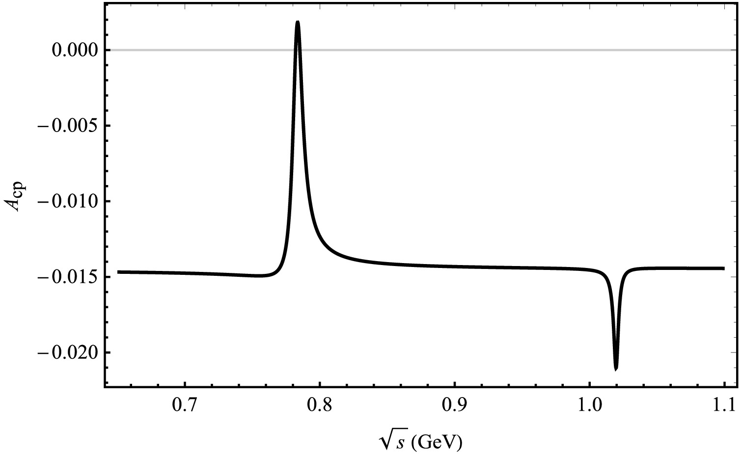
Figure 4. Plot of
$ A_{CP} $ as a function of$ \sqrt{s} $ corresponding to central parameter values of CKM matrix elements for the decay channel of$ B_{c}^{+} \rightarrow D_s^{+}\pi^{+}\pi^{-} $ .The maximum CP violation from the decay process
$ \ B_{c}^{+} \rightarrow D^{+}\pi^{+}\pi^{-} $ in Fig. 3, with a value of$ 97.54$ %, occurs at an invariant mass of 0.782 GeV, which corresponds to the mass of the ρ and ω mesons. Additionally, small peaks are also observed in the invariant mass range around the ϕ(1.02 GeV) meson. The value of CP violation is rather small, with a magnitude of$ 0.357$ %. In the decay process of$ \ B_{c}^{+} \rightarrow D^{+}\phi $ , only the contribution from the penguin diagram exists, while there is no contribution from the tree diagram. Hence, the$ \rho^0 -\omega $ mixing contributes considerably to the decay process.Regarding the decay process of
$ B_{c}^{+} \rightarrow D_s^{+}\pi^{+}\pi^{-} $ illustrated in Fig. 4, we observe a similar trend to$ B_{c}^{+} \rightarrow D^{+}\pi^{+}\pi^{-} $ . When the invariant mass of$ \pi^{+}\pi^{-} $ approaches that of the$ \rho^0 $ or ω, a pronounced peak is observed at approximately 0.783 GeV with a CP violation of$ 0.18$ %. Additionally, there is a smaller peak near the mass of the ϕ meson, corresponding to a value of$ -2.10$ %. -
In Fig. 5, we present the decay diagrams for the
$ B_{c}^{+} \rightarrow D_{(s)}^{+}\phi $ ($ \rho^0 $ , ω)$ \rightarrow D_{(s)}^{+}K^{+}K^{-} $ process. In these decay diagrams, the processes depicted in (a), (d), and (g) represent direct decay modes, where the$ K^{+} K^{-} $ pairs are produced via the intermediate states of$ \rho^0 $ , ω, and ϕ, respectively. Unlike the decay to$ \pi^{+} \pi^{-} $ meson pairs, all three vector mesons$ \rho^0 $ , ω, and ϕ can directly decay into$ K^{+} K^{-} $ meson pairs. In addition to the direct decay mechanism, the$ K^{+} K^{-} $ meson pair can also be generated through a mixing mechanism. Fig. 5(b), (c), (e), (f), (h), and (i) illustrate the contributions of the$ (\phi-\rho^0) $ ,$ (\phi-\omega) $ ,$ (\rho^0-\phi) $ ,$ (\rho^0-\omega) $ ,$ (\omega-\phi) $ , and$ (\omega-\rho^0) $ resonance hybrids, respectively. For instance, Fig. 5(b) demonstrates that the$ B_{c}^{+} $ meson decays into the$ D_{(s)}^{+} $ and ϕ mesons via quasi-two-body decay, followed by the resonant decay of the ϕ meson into a$ K^{+} K^{-} $ meson pair through mixing with the$ \rho^0 $ meson. Therefore, the$ K^{+} K^{-} $ meson pairs generated by this mixing mechanism correspond to six distinct cases. Although the contribution from this mixing mechanism is relatively small compared to direct decay, it is still significant and must be considered. Similar to the decay channel of$ B_{c}^{+} \rightarrow D_{(s)}^{+}\pi^{+}\pi^- $ , we provide the amplitude for$ B_{c}^{+} \rightarrow D_{(s)}^{+}K^{+}K^- $ :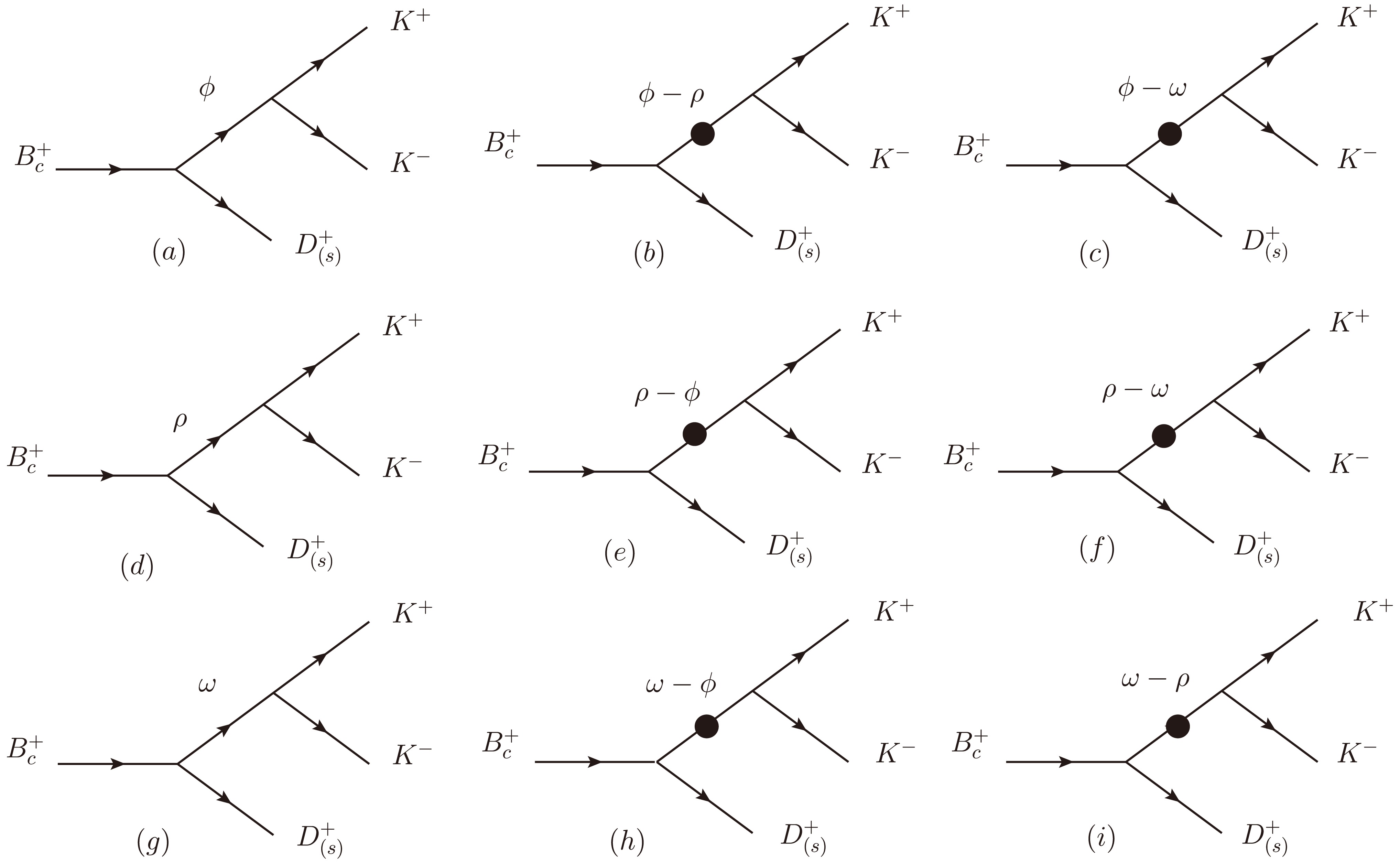
Figure 5. Decay diagrams of the
$ B_{c}^{+} \rightarrow D_{(s)}^{+}\phi $ ($ \rho^0 $ , ω)$ \rightarrow D_{(s)}^{+}K^{+}K^{-} $ process.$ \begin{split} &\quad\left \langle D_{(s)}^+K^+K^-\left | H^{T} \right | \ B_{c}^+ \right \rangle \\ &= \frac{g_{\phi\rightarrow K^+ K^-}}{s_{\phi}}t_{\phi} +\frac{g_{\rho\rightarrow K^+ K^-}}{s_{\rho}s_{\phi}}\widetilde{\Pi}_{\rho\phi}t_{\phi} +\frac{g_{\omega\rightarrow K^+ K^-}}{s_{\omega}s_{\phi}}\widetilde{\Pi}_{\omega\phi}t_{\phi} \\ &+\frac{g_{\rho\rightarrow K^+ K^-}}{s_{\rho}}t_{\rho} +\frac{g_{\phi\rightarrow K^+ K^-}}{s_{\phi}s_{\rho}}\widetilde{\Pi}_{\phi\rho}t_{\rho} +\frac{g_{\omega\rightarrow K^+ K^-}}{s_{\omega}s_{\rho}}\widetilde{\Pi}_{\omega\rho}t_{\rho}\\ & +\frac{g_{\omega\rightarrow K^+ K^-}}{s_{\omega}}t_{\omega} +\frac{g_{\phi\rightarrow K^+ K^-}}{s_{\phi}s_{\omega}}\widetilde{\Pi}_{\phi\omega}t_{\omega}+\frac{g_{\rho\rightarrow K^+ K^-}}{s_{\rho}s_{\omega}}\widetilde{\Pi}_{\rho\omega}t_{\omega}, \end{split} $

(12) $ \begin{split} &\quad\left \langle D_{(s)}^+K^+K^-\left | H^{P} \right | \ B_{c}^+ \right \rangle \\ &= \frac{g_{\phi\rightarrow K^+ K^-}}{s_{\phi}}p_{\phi} +\frac{g_{\rho\rightarrow K^+ K^-}}{s_{\rho}s_{\phi}}\widetilde{\Pi}_{\rho\phi}p_{\phi} +\frac{g_{\omega\rightarrow K^+ K^-}}{s_{\omega}s_{\phi}}\widetilde{\Pi}_{\omega\phi}p_{\phi}\\ & +\frac{g_{\rho\rightarrow K^+ K^-}}{s_{\rho}}p_{\rho} +\frac{g_{\phi\rightarrow K^+ K^-}}{s_{\phi}s_{\rho}}\widetilde{\Pi}_{\phi\rho}p_{\rho} +\frac{g_{\omega\rightarrow K^+ K^-}}{s_{\omega s_{\rho}}}\widetilde{\Pi}_{\omega\rho}p_{\rho}\\ & +\frac{g_{\omega\rightarrow K^+ K^-}}{s_{\omega}}p_{\omega} +\frac{g_{\phi\rightarrow K^+ K^-}}{s_{\phi}s_{\omega}}\widetilde{\Pi}_{\phi\omega}p_{\omega} +\frac{g_{\rho\rightarrow K^+ K^-}}{s_{\rho}s_{\omega}}\widetilde{\Pi}_{\rho\omega}p_{\omega}. \end{split} $

(13) Here,
$ g_{V} $ denotes the coupling constant obtained from the decay process$ V \rightarrow K^{+} K^{-} $ . Moreover, the following relationship holds:$ \sqrt{2}g_{{\rho}K^{+} K^{-}} = \sqrt{2}g_{\omega K^{+} K^{-}} = -g_{\phi K^{+} K^{-}} = 4.54 $ [31, 32]. -
Figure 5 illustrates nine distinct scenarios in the decay process
$ B_{c}^{+} \rightarrow D_{(s)}^{+}K^{+}K^- $ . Among these, (b), (d), and (i) closely resemble the decay process of$ B_{c}^{+} \rightarrow D_{(s)}^{+}\pi^{+}\pi^- $ , differing only by the substitution of π with K. The amplitude forms for these cases are similar to those presented in Eqs. (13)−(18). Focusing on the$ B_{c}^{+} \rightarrow D^{+}K^{+}K^- $ decay process as an example, we outline all corresponding amplitude forms depicted in Fig. 5. These forms sequentially correspond to Fig. 5 (a), (e), (h), (g), (c), and (f):$ \begin{aligned}[b] & A\left(\ B_{c}^+ \rightarrow\right.\left. D^+\phi\rightarrow D^+K^+K^-\right) = \frac{<D^+\phi|H_{\rm eff}|B_{c}^+><K^+K^-|H_{\phi \rightarrow K^+K^- }|\phi>}{({s-m_{\phi}^{2}+{\rm i}\,m_{\phi} \varGamma_{\phi}})} = \sum\limits_{\lambda = 0,\pm 1} \frac{G_{F}P_{B_{c}^+}\cdot \epsilon^*\left( \lambda \right)\ g^{\phi \rightarrow K^+K^- }\epsilon \left( \lambda \right) \cdot \left( p_{K ^+}-p_{K ^-} \right)}{\sqrt{2}({s-m_{\phi}^{2}+{\rm i}\,m_{\phi} \varGamma_{\phi}})} \\ &\quad \times \bigg\{-V_{u d} V_{u b}^{*}\left[(C_4-\frac{1}{2}C_{10}){\cal{M}}_{e}^{LL}+(C_6-\frac{1}{2}C_8){\cal{M}}_{e}^{SP}+(C_3+\frac{1}{3}C_4\right.\left.-\frac{1}{2}C_9-\frac{1}{6}C_{10}){F}_{e}^{LL}+(C_5+\frac{1}{3}C_6-\frac{1}{2}C_7-\frac{1}{6}C_8){F}_{e}^{LR}\right]\bigg\}, \end{aligned} $

(14) $ \begin{aligned}[b]& \sqrt{2}A\left(\ B_{c}^+ \rightarrow\right.\left. D^+(\rho^{0}-\phi)\rightarrow D^+K^+K^-\right) = \frac{<D^+\rho ^0|H_{\rm eff}|B_{c}^+><K^+K^-|H_{\phi\rightarrow K^+K^- }|\phi>\widetilde{\Pi}_{\phi\rho}}{({s-m_{\rho ^0}^{2}+{\rm i}\,m_{\rho ^0} \varGamma _{\rho ^0}})({s-m_{\phi}^{2}+{\rm i}\,m_{\phi} \varGamma_{\phi}})}\\ =\;& \sum\limits_{\lambda = 0,\pm 1} \frac{G_{F}P_{B_{c}^+}\cdot \epsilon^*\left( \lambda \right)\ g^{\phi\rightarrow K^+K^- }\epsilon \left( \lambda \right) \cdot \left( p_{K ^+}-p_{K ^-} \right)\widetilde{\Pi}_{\phi\rho}}{\sqrt{2}{({s-m_{\rho ^0}^{2}+{\rm i}\,m_{\rho ^0} \varGamma _{\rho ^0}}})({s-m_{\phi}^{2}+{\rm i}\,m_{\phi} \varGamma_{\phi}})} \left.\times \Bigg\{V_{u d} V_{u b}^{*}\left[F_{e}^{L L}(C_1+\frac{1}{3}C_2)+M_{e}^{L L}(C_{2})+F_{a}^{L L }(C_{2}+\frac{1}{3}C_1)+M_{a}^{L L}(C_{1})\right] \right.\\&+ V_{t d} V_{t b}^{*}\bigg\{F_{a}^{L L}(C_{2}+\frac{1}{3}C_1)+M_{a}^{L L}(C_{1})-\left[{\cal{M}}_{e}^{LL}(\frac{3}{2}C_{10}-C_3+\frac{1}{2}C_9)\right.-M_{a}^{L L}(C_{3}+C_{9})+M_{e}^{L R}(-C_{5}+\frac{1}{2}C_{7})\\&+(-C_4-\frac{1}{3}C_3-C_{10}-\frac{1}{3}C_9){F}_a^{LL}+(C_{10}+\frac{5}{3}C_9-\frac{1}{3}C_3-C_4-\frac{3}{2}C_7-\frac{1}{2}C_8){F}_e^{LL}\\ &\left.+(-C_6-\frac{1}{3}C_5+\frac{1}{2}C_{8}+\frac{1}{6}C_7){F}_e^{SP}-(C_5+C_7){\cal{M}}_a^{LR}\right.\left.+(-C_6-\frac{1}{3}C_5-C_{8}-\frac{1}{3}C_7) {F}_a^{SP}\right]\bigg\}\Bigg\}, \end{aligned} $

(15) $ \begin{aligned}[b]& \sqrt{2}A\left(\ B_{c}^+ \rightarrow\right.\left. D^+(\omega-\phi)\rightarrow D^+K^+K^-\right) = \frac{<D^+\omega|H_{\rm eff}|B_{c}^+><K^+K^-|H_{\phi\rightarrow K^+K^- }|\phi>\widetilde{\Pi}_{\phi\omega}}{({s-m_{\omega}^{2}+{\rm i}\,m_{\omega} \varGamma_{\omega}})({s-m_{\phi}^{2}+{\rm i}\,m_{\phi} \varGamma_{\phi}})} \\ =\;& \sum\limits_{\lambda = 0,\pm 1} \frac{G_{F}P_{B_{c}^+}\cdot \epsilon^*\left( \lambda \right)\ g^{\phi\rightarrow K^+K^- }\epsilon \left( \lambda \right) \cdot \left( p_{K ^+}-p_{K ^-} \right)\widetilde{\Pi}_{\phi\omega}}{\sqrt{2}({s-m_{\omega}^{2}+{\rm i}\,m_{\omega} \varGamma_{\omega}})({s-m_{\phi}^{2}+{\rm i}\,m_{\phi} \varGamma_{\phi}})}\left.\times \bigg\{V_{u d} V_{u b}^{*}\left[ F_{e}^{L L}\left(c_{1}+\frac{1}{3}C_2\right)+C_2{\cal{M}}_{e}^{LL}-\left((C_2+\frac{1}{3}C_1)F_{a}^{L L}+C_1{\cal{M}}_{a}^{LL}\right)\right]\right.\\ &\left.-V_{t d} V_{t b}^{*}\left[(C_2+\frac{1}{3}C_1)F_{a}^{L L}+C_1{\cal{M}}_{a}^{LL}+\left((2C_4+C_3+\frac{1}{2}C_{10}-\frac{1}{2}C_9){\cal{M}}_{e}^{LL}\right)\right.\right.+(C_3+C_9){\cal{M}}_{e}^{LL}+(C_5-\frac{1}{2}C_7){\cal{M}}_{e}^{LR}\\ &+(C_5+C_7){\cal{M}}_{a}^{LR}+(C_4+\frac{1}{3}C_3+C_{10}+\frac{1}{3}C_9) {F}_{a}^{LL}+(\frac{7}{3}C_3+\frac{5}{3}C_4+\frac{1}{3}(C_9-C_{10})){F}_{e}^{LL}+(2C_5+\frac{2}{3}C_6+\frac{1}{2}C_7+\frac{1}{6}C_8){F}_{e}^{LR}\\ &+(C_6+\frac{1}{3}C_5-\frac{1}{2}C_{8}-\frac{1}{6}C_7){F}_{e}^{SP}\left.+(C_6+\frac{1}{3}C_5+C_{8}+\frac{1}{3}C_7){F}_{a}^{SP}\right]\bigg\}, \end{aligned} $

(16) $ \begin{aligned}[b] & \sqrt{2}A\left(\ B_{c}^+ \rightarrow\right.\left. D^+\omega\rightarrow D^+K^+K^-\right) = \frac{<D^+\omega|H_{\rm eff}|B_{c}^+><K^+K^-|H_{\omega\rightarrow K^+K^- }|\omega>}{({s-m_{\omega}^{2}+{\rm i}\,m_{\omega} \varGamma_{\omega}})} \\ =\;& \sum\limits_{\lambda = 0,\pm 1} \frac{G_{F}P_{B_{c}^+}\cdot \epsilon^*\left( \lambda \right)\ g^{\omega\rightarrow K^+K^- }\epsilon \left( \lambda \right) \cdot \left( p_{K ^+}-p_{K ^-} \right)}{\sqrt{2}({s-m_{\omega}^{2}+{\rm i}\,m_{\omega} \varGamma_{\omega}})}\left.\times \bigg\{V_{u d} V_{u b}^{*}\left[ F_{e}^{L L}\left(c_{1}+\frac{1}{3}C_2\right)+C_2{\cal{M}}_{e}^{LL}-\left((C_2+\frac{1}{3}C_1)F_{a}^{L L}+C_1{\cal{M}}_{a}^{LL}\right)\right]\right.\\&\left.-V_{t d} V_{t b}^{*}\left[(C_2+\frac{1}{3}C_1)F_{a}^{L L}+C_1{\cal{M}}_{a}^{LL}+\left((2C_4+C_3+\frac{1}{2}C_{10}-\frac{1}{2}C_9){\cal{M}}_{e}^{LL}\right)\right.\right.+(C_3+C_9){\cal{M}}_{e}^{LL}+(C_5-\frac{1}{2}C_7){\cal{M}}_{e}^{LR}\\&+(C_5+C_7){\cal{M}}_{a}^{LR}\left.+(C_4+\frac{1}{3}C_3+C_{10}+\frac{1}{3}C_9) {F}_{a}^{LL}+(\frac{7}{3}C_3+\frac{5}{3}C_4+\frac{1}{3}(C_9-C_{10})){F}_{e}^{LL}\right.+(2C_5+\frac{2}{3}C_6+\frac{1}{2}C_7+\frac{1}{6}C_8){F}_{e}^{LR}\\&+(C_6+\frac{1}{3}C_5-\frac{1}{2}C_{8}-\frac{1}{6}C_7){F}_{e}^{SP}\left.+(C_6+\frac{1}{3}C_5+C_{8}+\frac{1}{3}C_7){F}_{a}^{SP}\right]\bigg\}, \end{aligned} $

(17) $ \begin{aligned}[b]& A\left(\ B_{c}^+ \rightarrow\right.\left. D^+(\phi-\omega)\rightarrow D^+K^+K^-\right) = \frac{<D^+\phi|H_{\rm eff}|B_{c}^+><K^+K^-|H_{\omega\rightarrow K^+K^- }|\omega>\widetilde{\Pi}_{\omega\phi}}{({s-m_{\phi}^{2}+{\rm i}\,m_{\phi} \varGamma_{\phi}})({s-m_{\omega}^{2}+{\rm i}\,m_{\omega} \varGamma_{\omega}})} \\ =\;& \sum\limits_{\lambda = 0,\pm 1} \frac{G_{F}P_{B_{c}^+}\cdot \epsilon^*\left( \lambda \right)\ g^{\omega\rightarrow K^+K^- }\epsilon \left( \lambda \right) \cdot \left( p_{K ^+}-p_{K ^-} \right)\widetilde{\Pi}_{\omega\phi}}{\sqrt{2}({s-m_{\phi}^{2}+{\rm i}\,m_{\phi} \varGamma_{\phi}})({s-m_{\omega}^{2}+{\rm i}\,m_{\omega} \varGamma_{\omega}})} \times \bigg\{-V_{u d} V_{u b}^{*}\left[(C_4-\frac{1}{2}C_{10}){\cal{M}}_{e}^{LL}+(C_6-\frac{1}{2}C_8){\cal{M}}_{e}^{SP}\right.\\&+(C_3+\frac{1}{3}C_4\left.-\frac{1}{2}C_9-\frac{1}{6}C_{10}){F}_{e}^{LL}+(C_5+\frac{1}{3}C_6-\frac{1}{2}C_7-\frac{1}{6}C_8){F}_{e}^{LR}\right]\bigg\}, \end{aligned} $

(18) and
$ \begin{aligned}[b]& \sqrt{2}A\left(\ B_{c}^+ \rightarrow\right.\left. D^+(\rho^{0}-\omega)\rightarrow D^+K^+K^-\right) = \frac{<D^+\rho ^0|H_{\rm eff}|B_{c}^+><K^+K^-|H_{\omega\rightarrow K^+K^-}|\omega>\widetilde{\Pi}_{\omega\rho}}{({s-m_{\rho ^0}^{2}+{\rm i}\,m_{\rho ^0} \varGamma _{\rho ^0}})({s-m_{\omega}^{2}+{\rm i}\,m_{\omega} \varGamma_{\omega}})}\\ =\;& \sum\limits_{\lambda = 0,\pm 1} \frac{G_{F}P_{B_{c}^+}\cdot \epsilon^*\left( \lambda \right)\ g^{\omega\rightarrow K^+K^- }\epsilon \left( \lambda \right) \cdot \left( p_{K ^+}-p_{K ^-} \right)\widetilde{\Pi}_{\omega\rho}}{\sqrt{2}{({s-m_{\rho ^0}^{2}+{\rm i}\,m_{\rho ^0} \varGamma _{\rho ^0}}})({s-m_{\omega}^{2}+{\rm i}\,m_{\omega} \varGamma_{\omega}})} \left.\times \Bigg\{V_{u d} V_{u b}^{*}\left[F_{e}^{L L}(C_1+\frac{1}{3}C_2)+M_{e}^{L L}(C_{2})+F_{a}^{L L }(C_{2}+\frac{1}{3}C_1)+M_{a}^{L L}(C_{1})\right] \right.\\ &+ V_{t d} V_{t b}^{*}\bigg\{F_{a}^{L L}(C_{2}+\frac{1}{3}C_1)+M_{a}^{L L}(C_{1})-\left[{\cal{M}}_{e}^{LL}(\frac{3}{2}C_{10}-C_3+\frac{1}{2}C_9)\right.-M_{a}^{L L}(C_{3}+C_{9})+M_{e}^{L R}(-C_{5}+\frac{1}{2}C_{7})\\&+(-C_4-\frac{1}{3}C_3-C_{10}-\frac{1}{3}C_9){F}_a^{LL}\left.+(C_{10}+\frac{5}{3}C_9-\frac{1}{3}C_3-C_4-\frac{3}{2}C_7-\frac{1}{2}C_8){F}_e^{LL}\right.+(-C_6-\frac{1}{3}C_5+\frac{1}{2}C_{8}+\frac{1}{6}C_7){F}_e^{SP}\\ &-(C_5+C_7){\cal{M}}_a^{LR}\left.+(-C_6-\frac{1}{3}C_5-C_{8}-\frac{1}{3}C_7) {F}_a^{SP}\right]\bigg\}\Bigg\}. \end{aligned} $

(19) -
We present plots illustrating CP violation in the decay processes of
$ B_{c}^{+} \rightarrow D^{+}K^{+}K^{-} $ and$ B_{c}^{+} \rightarrow D_s^{+}K^{+}K^{-} $ . Taking into account the$ K^{+}K^{-} $ threshold, Figs. 6 and 7 depict the variation of$ A_{\rm CP} $ as a function of$ \sqrt{s} $ , representing the invariant mass of the$ K^{+}K^{-} $ system. In the decay process of$ B_{c}^{+} \rightarrow D^{+}K^{+}K^{-} $ shown in Fig. 6, a pronounced CP-violating effect is observed near 1.02 GeV. The peak value reaches$ 34.30$ % when the invariant mass of$ K^+K^- $ is close to the mass of the ϕ meson (1.02 GeV). In the decay process of$ B_{c}^{+} \rightarrow D^{+}\phi $ associated with the$ B_{c}^{+} \rightarrow D^{+}K^{+}K^{-} $ decay, it is observed that only the penguin diagram contributes, while there is no contribution from the tree diagram, which does not induce CP violation. The CP violation depends on the intermediate decay processes$ \rho \rightarrow K^{+}K^{-} $ and$ \omega \rightarrow K^{+}K^{-} $ , as well as the interference between these processes and$ \phi \rightarrow K^{+}K^{-} $ .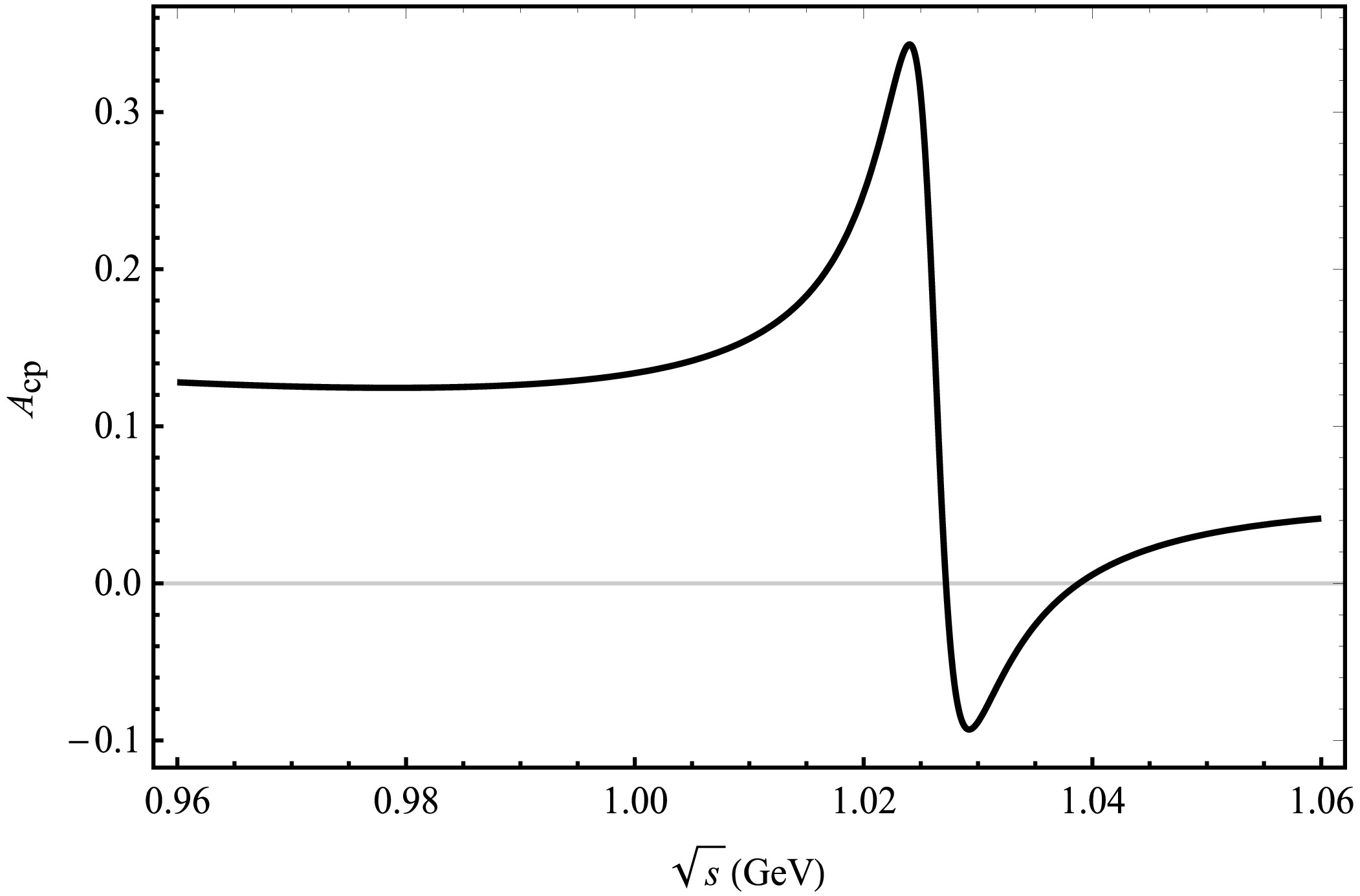
Figure 6. Plot of
$ A_{\rm CP} $ as a function of$ \sqrt{s} $ corresponding to central parameter values of CKM matrix elements for the decay channel of$ B_{c}^{+} \rightarrow D^{+}K^{+}K^{-} $ .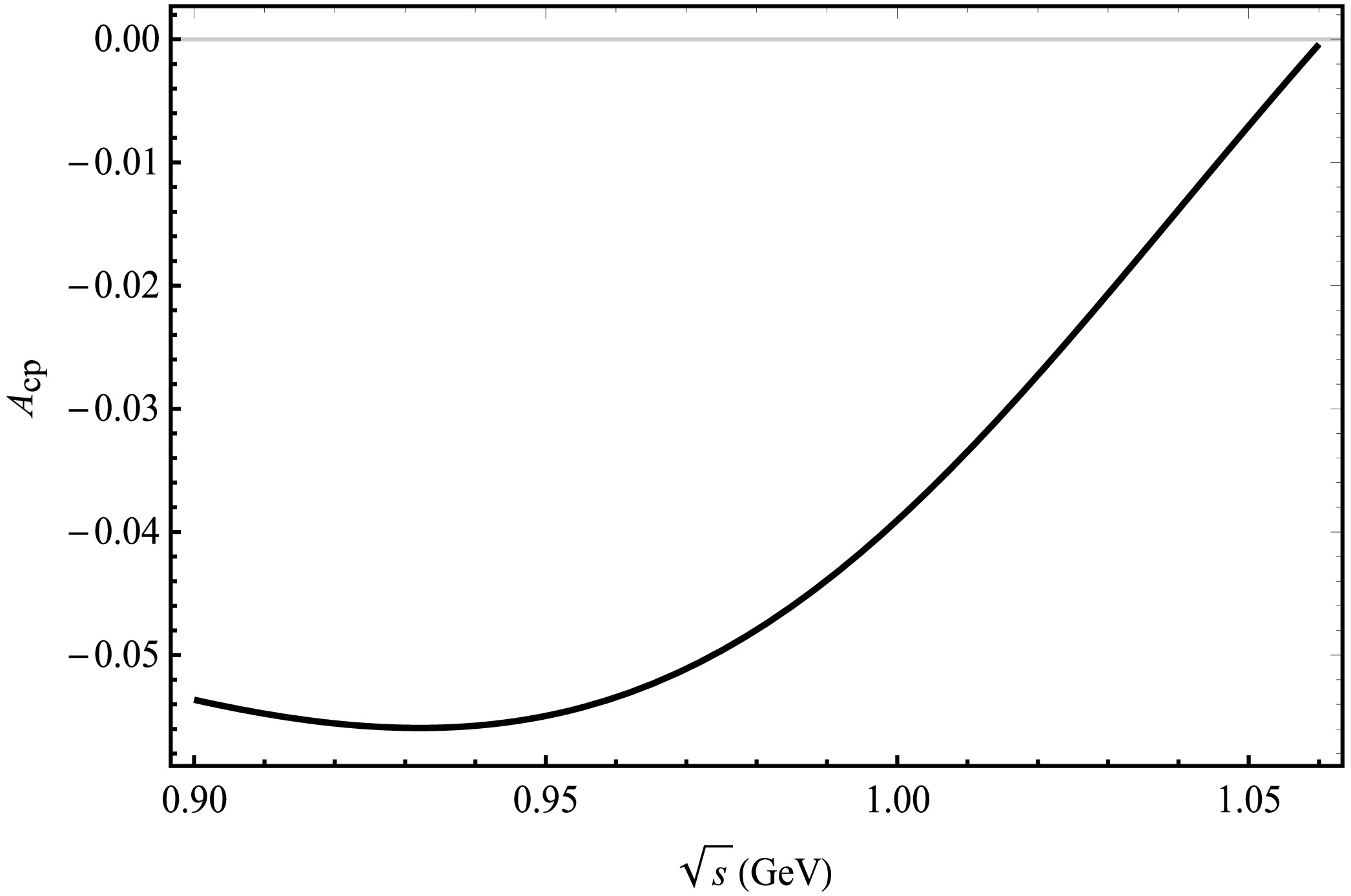
Figure 7. Plot of
$ A_{\rm CP} $ as a function of$ \sqrt{s} $ corresponding to central parameter values of CKM matrix elements for the decay channel of$ B_{c}^{+} \rightarrow D_s^{+}K^{+}K^{-} $ .In the decay process of
$ B_{c}^{+} \rightarrow D_s^{+}K^{+}K^{-} $ shown in Fig. 7, an intriguing phenomenon has been observed. The CP violation exhibits a sharp increase when the invariant mass of the$ K^+K^- $ pair is around 0.93 GeV. Notably, this peak does not align with the mass of the ϕ meson; instead, it spans a broader range from 0.9 to 1.05 GeV. We propose that this behavior results from the resonant mixing of the$ \rho^0 $ , ω, and ϕ particles, with the decay channel$ \phi \rightarrow K^{+}K^{-} $ making the dominant contribution through its combined effect. -
In this paper, we perform the integral calculation of
$ A_{\rm CP} $ to facilitate future experimental comparisons. For the decay process$ B_{c}^{+} \rightarrow D_{(s)}^{+}\rho^0 $ , the amplitude is given by$ M_{\ B_{c}^{+}\rightarrow D_{(s)}^{+}\rho^0}^{\lambda} = \alpha p_{B_{c}^{+}} \cdot \epsilon^{*}(\lambda) $ , where$ p_{B_{c}^{+}} $ represents the momenta of the$ B_{c}^{+} $ meson, ϵ denotes the polarization vector of$ \rho^0 $ , and λ corresponds to its polarization. The parameter α remains independent of λ, which is from the contribution of PQCD. Similarly, in the decay process$ \rho^0 \rightarrow \pi^{+}\pi^{-} $ , we can express$ M_{\rho^0 \rightarrow \pi^{+}\pi^{-}}^{\lambda} = g_{\rho}\epsilon(\lambda)\left(p_1-p_2\right) $ , where$ p_1 $ and$ p_2 $ denote the momenta of the produced$ \pi^{+} $ and$ \pi^{-} $ particles from$ \rho^0 $ meson, respectively. Here, the parameter$ g_\rho $ represents an effective coupling constant for$ \rho^0 \rightarrow \pi^{+}\pi^{-} $ . Regarding the dynamics of meson decay, it is observed that the polarization vector of a vector meson satisfies$ \sum\nolimits_{\lambda = 0,\pm 1}\epsilon^\lambda_\mu(p)(\epsilon^\lambda_\nu(p))^* = -(g_{\mu\nu}-p_\mu p_\nu/m_V^2) $ . As a result, we obtain the total amplitude for the decay process$ B_{c}^{+} \rightarrow D_{(s)}^{+}\rho^0\rightarrow D_{(s)}^{+}\pi^{+}\pi^- $ [30]:$ \begin{aligned}[b] A =\;& \alpha p_{\ B_{c}^+}^{\mu} \frac{\sum\nolimits_{\lambda} \epsilon_{\mu}^{*}(\lambda) \epsilon_{\nu}(\lambda)}{s_{\rho}} g_{\rho \pi\pi}\left(p_{1}-p_{2}\right)^{\nu} \\ =\;& \frac{g_{\rho \pi\pi} \alpha}{s_{\rho}} \cdot p_{\ B_{c}^+}^{\mu}\left[g_{\mu \nu}-\frac{\left(p_{1}+p_{2}\right)_{\mu}\left(p_{1}+p_{2}\right)_{\nu}}{s}\right]\left(p_{1}-p_{2}\right)^{\nu} \\ =\;& \frac{g_{\rho \pi\pi}}{s_{\rho}} \cdot \frac{M_{\ B_{c}^+\rightarrow \rho^0 D_{(s)}^+}^{\lambda}}{p_{\ B_{c}^+} \cdot \epsilon^{*}} \cdot\left(\Sigma-s^{\prime}\right) \\ =\;& \left(\Sigma-s^{\prime}\right) \cdot {\cal{A}}. \end{aligned} $

(20) The high (
$ \sqrt{s^\prime} $ ) and low$ \sqrt{s} $ ranges are defined for calculating the invariant mass of$ \pi^{+} \pi^{-} $ . By setting a fixed value for s, we can determine an appropriate value for$ s^\prime $ that fulfills the equation$ \Sigma = \frac{1}{2}\left(s_{\max }^\prime+s_{\min }^\prime\right) $ , where$ { s}_{ \max }^{ \prime }( { s}_{ \min }^{\prime}) $ denotes the maximum (minimum) value.Utilizing the principles of three-body kinematics, we can deduce the local CP asymmetry for the decay
$ B_{c}^{+} \rightarrow D_{(s)}^{+}\pi^{+}\pi^- $ within a specific range of invariant mass:$ A_{C P}^{\Omega} = \frac{\displaystyle\int_{s_{1}}^{s_{2}} \mathrm{\; d} s \displaystyle\int_{s_{1}^{\prime}}^{s_{2}^{\prime}} \mathrm{d} s^{\prime}\left(\Sigma-s^{\prime}\right)^{2}\left(|{\cal{A}}|^{2}-|\overline{{\cal{A}}}|^{2}\right)}{\displaystyle\int_{s_{1}}^{s_{2}} \mathrm{\; d} s \displaystyle\int_{s_{1}^{\prime}}^{s_{2}^{\prime}} \mathrm{d} s^{\prime}\left(\Sigma-s^{\prime}\right)^{2}\left(|{\cal{A}}|^{2}+|\overline{{\cal{A}}}|^{2}\right)}. $

(21) Our calculation takes into account the dependence of
$ \Sigma = \dfrac{1}{2}\left(s_{\max }^{\prime}+s_{\min }^{\prime}\right) $ on$ s^{\prime} $ . Assuming that$ s_{\max }^{\prime}>s^{\prime}>s_{\min }^{\prime} $ represents an integral interval of high invariant mass for the$ \pi^{+} \pi^{-} $ meson pair and$ \int_{s_{1}^{\prime}}^{s_{2}^{\prime}} \mathrm{d}s^\prime(\Sigma-s')^{2} $ represents a factor dependent on$ s' $ , the correlation between Σ and$ s' $ can be easily determined through kinematic analysis, as$ s' $ only varies on a small scale. Therefore, we can consider Σ as a constant. This allows us to cancel out the term$ \int_{s_1^\prime}^{ s_2^\prime }\mathrm{d}s^\prime (\Sigma-s')^{2} $ in both the numerator and denominator, resulting in$ A_{\rm CP}^{\Omega} $ no longer depending on the high invariant mass of positive and negative particles. The form of$ B_{c}^{+} \rightarrow D_{(s)}^{+}\phi $ ($ \rho^0 $ , ω)$ \rightarrow D_{(s)}^{+}K^{+}K^{-} $ is similar to that of$ B_{c}^{+} \rightarrow D_{(s)}^{+}\rho^{0} $ (ω, ϕ)$ \rightarrow D_{(s)}^{+}\pi^{+}\pi^{-} $ , and only π needs to be replaced with K. -
According to Table 1, the integration ranges of 0.65 GeV to 1.06 GeV and 0.98 GeV to 1.06 GeV correspond to the resonance regions for the
$ \pi^{+}\pi^{-} $ and$ K^{+}K^{-} $ final states, respectively. The threshold for the$ K^{+}K^{-} $ final state is also considered. The resonance interactions between different particles can result in more pronounced CP violation phenomena across various energy intervals. We present the local integral values in Table 1. We have comparatively analyzed the distinctions between the three-particle mixed resonance of$ \rho^0 -\omega-\phi $ and the two-particle mixed resonances of$ \rho^0 -\omega $ ,$ \phi-\rho^0 $ and$ \phi-\omega $ , while also providing numerical results that exclude these mixed resonances.Decay channel $ B_{c}^{+} \rightarrow D^{+}\pi^{+}\pi^{-}$ 

$ B_{c}^{+} \rightarrow D_s^{+}\pi^{+}\pi^{-}$ 

$ B_{c}^{+} \rightarrow D^{+}K^{+}K^{-}$ 

$ B_{c}^{+} \rightarrow D_s^{+}K^{+}K^{-}$ 

$\phi-\rho-\omega$ mixing

$\mathrm{0.0706^{+0.002-0.063}_{-0.002-0.091} }$ 

$\mathrm{-0.0134^{+0.0005-0.0016}_{-0.0005+0.0006} } $ 

$ \mathrm{0.1636^{+0.006+0.046}_{-0.006-0.067} }$ 

$ \mathrm{-0.0278^{+0.001-0.0004}_{-0.001+0.0012} }$ 

$\rho-\omega$ mixing

$\mathrm{0.0706^{+0.002-0.064}_{-0.002-0.091} } $ 

$\mathrm{-0.0133^{+0.0005-0.0013}_{-0.0005+0.0012} } $ 

$ \mathrm{0.0906^{+0.006+0.074}_{-0.006-0.072} }$ 

$ \mathrm{-0.0267^{+0.001+0.014}_{-0.001-0.004} }$ 

$\phi-\rho$ mixing

$\mathrm{-0.0176^{+0.0006+0}_{-0.0006-0} }$ 

$\mathrm{-0.0156^{+0.0006-0.0005}_{-0.0006+0.00001} }$ 

$\mathrm{0.0290^{+0.0005-0.045}_{-0.0005-0.041} }$ 

$ \mathrm{-0.0258^{+0.0009+0.0012}_{-0.0009+0.0008} }$ 

$\phi-\omega$ mixing

$ \mathrm{-}$ 

$\mathrm{-}$ 

$\mathrm{-0.0381^{+0.0006+0.012}_{-0.0006-0.0096} }$ 

$ \mathrm{-0.0264^{+0.00003-0.002}_{-0.00003-0.001} }$ 

no mixing $ \mathrm{-0.0176^{+0.0006+0}_{-0.0006-0} }$ 

$\mathrm{-0.0155^{+0.0006+0}_{-0.0006-0} }$ 

$\mathrm{0.0784^{+0.001+0.091}_{-0.001+0.050} }$ 

$ \mathrm{-0.0252^{+0.0009+0.0015}_{-0.0009+0.0005} }$ 

Table 1. Peak local integral (
$0.65$ $ \mathrm{\mathrm{ }}\mathrm{GeV}\le\sqrt{s}\le1.06 $ $ \mathrm{GeV} $ for the$\pi^{+}\pi^{-}$ final states and$0.98$ $ \mathrm{GeV}\le\sqrt{s}\le1.06 $ $ \mathrm{GeV} $ for the$K^{+}K^{-}$ final states) of$\mathrm{A}^{\Omega} _{\mathrm{CP}}$ from different resonance ranges for$ B_{c}^{+} \rightarrow D_{(s)}^{+}\pi^{+}\pi^-$ and$ B_{c}^{+} \rightarrow D_{(s)}^{+}K^{+}K^-$ decay processes.During the decay process of
$ B_{c}^{+} \rightarrow D^{+}\pi^{+}\pi^{-} $ , both in the case of a three-particle mixture and$ \rho^0 - \omega $ mixture, the variation of CP violation is significantly larger in the resonant region compared to the non-resonant scenario, with changes in sign. Despite a peak reaching$ 97.54$ % of CP violation, the local integral value exhibits only minor fluctuations, and the central value of$ \mathrm{A}^{\Omega}_{\mathrm{CP}} $ is approximately 0.0706. The influence of$ \phi-\rho^0 $ mixing is relatively insignificant compared to the no-mixing results. Additionally, the effect of$ \phi-\omega $ mixing, arising from higher-order contributions with very small values, can be neglected. Therefore, we do not present these results. For the$ B_{c}^{+} \rightarrow D^{+}\pi^{+}\pi^{-} $ and$ B_{c}^{+} \rightarrow D_s^{+}\pi^{+}\pi^{-} $ decay processes, the outcome of "no mixing" is depicted in Fig. 1(a), namely, it is the result of the direct decay of$ B_{c}^{+} \rightarrow D^{+}\rho^0 \rightarrow D^{+}\pi^{+}\pi^{-} $ . The outcome of this process is –0.0176. Meanwhile, we also computed the result of the process represented by Fig. 1(c), and the result was –0.0106. In other words, the$ \rho-\omega $ mixing mechanism significantly influences the total CP violation. For the decay processes of$ B_{c}^{+} \rightarrow D_s^{+}\pi^{+}\pi^{-} $ , the three-particle mixing mechanism exhibits negligible effects on CP violation. In the decay processes of both$ B_{c}^{+} \rightarrow D^{+}\pi^{+}\pi^{-} $ and$ B_{c}^{+} \rightarrow D_s^{+}\pi^{+}\pi^{-} $ , the values of the$ \rho^0 - \omega - \phi $ mixing and$ \rho^0 - \omega $ mixing are essentially identical. The influence of$ \phi - \rho^0 $ mixing is relatively minor and can be disregarded.The effect of the mixing mechanism in the decay process of
$ B_{c}^{+} \rightarrow D^{+}K^{+}K^{-} $ is significant, with the central value of$ \mathrm{A}^{\Omega}_{\mathrm{CP}} $ reaching 0.1636 for CP violation, compared to 0.0784 without mixing. This is because, in the decay process of$ B_{c}^{+} \rightarrow D^{+}\phi $ , only the penguin diagram contributes, while there is no contribution from the tree diagram. Consequently, considering the three-particle mixing, the change in CP violation becomes more pronounced. However, in the process$ B_{c}^{+} \rightarrow D_s^{+}K^{+}K^{-} $ , the CP violation exhibits a notable increase due to the three-particle mixing.Theoretical errors give rise to uncertainties in the results. In general, the major theoretical uncertainties arise from power corrections beyond the heavy quark limit, necessitating the inclusion of
$ 1/m_b $ power corrections. However, the$ 1/m_b $ corrections are power-suppressed and typically non-perturbative, meaning that they cannot be accurately calculated using perturbation theory. Consequently, this scheme introduces additional sources of uncertainty. The first source of error comes from variations in CKM parameters, while the second comes from hadronic parameters such as mixing parameters, form factors, decay constants,$ B_c $ meson wave functions, and D meson wave functions. By employing central values for these parameters, we initially compute numerical results for CP violation and subsequently incorporate errors based on standard deviations, as shown in Table 1. -
Due to isospin breaking, the effects of three-particle mixing on the branching ratios of
$ B_{c}^{+} \rightarrow D_{(s)}^{+}\rho^{0} \rightarrow D_{(s)}^{+}\pi^{+}\pi^{-} $ are symmetrical. By considering$ \sqrt{2}g_{{\rho}K^{+} K^{-}} = \sqrt{2}g_{\omega K^{+} K^{-}} = -g_{\phi K^{+} K^{-}} = 4.54 $ , we calculate the branching ratios of$ B_{c}^{+} \rightarrow D_{(s)}^{+}V \rightarrow D_{(s)}^{+}K^{+}K^{-} $ both with and without three-particle mixing. The differential branching ratio for the quasi-two-body$ B_{c}^{+} \rightarrow D_{(s)}^{+}V \rightarrow D_{(s)}^{+}K^{+}K^{-} $ decays is written as [33, 34]$ \frac{{\rm d}{{\cal{B}}}}{{\rm d}\zeta} = \frac{\tau_{B_{c}} \, q^3_{D_{(s)}^+} \, q^3}{48 \, \pi^3 \, m^5_{B_{c}}} \, \overline{\vert {{\cal{A}}} \vert^2} \,, $

(22) with the variable
$ {\zeta} = \dfrac{s}{m_{B_{c}}^2} $ and$ B_c $ meson mean lifetime$ \tau_{B_{c}} $ . Among them, q and$ q_{D_{(s)}^{+}} $ are respectively defined as$ q = \frac{1}{2} \sqrt{ s-(m_K+m_K)^2}, $

(23) and
$ q_{D_{(s)}^+} = \frac{1}{2}\sqrt{\big[\left(m^2_{B}-m_{D_{(s)}^+}^2\right)^2 -2\left(m^2_{B}+m_{D_{(s)}^+}^2\right)s+s^2\big]/s} \,. $

(24) The formula for computing
$ B_{c}^{+} \rightarrow D_{(s)}^{+}V \rightarrow D_{(s)}^{+}\pi^{+}\pi^{-} $ merely requires substituting$ m_K $ with$ m_\pi $ into Eq. (23). In calculating the decays of$ B_{c}^{+} \rightarrow D_{(s)}^{+}\rho^0 \rightarrow D_{(s)}^{+}K^{+}K^{-} $ and$ B_{c}^{+} \rightarrow D_{(s)}^{+}\omega \rightarrow D_{(s)}^{+}K^{+}K^{-} $ , the$ \rho^0 $ and ω pole masses are below the invariant mass threshold, i.e.,$ m_\rho(\omega) < m_K + m_K $ [35]. In this case, the pole mass of$ m_\rho(\omega) $ should be replaced by an effective mass$ m_0^{\text{eff}} $ to avoid kinematic singularities in the phase space factor [36]:$ \begin{aligned}[b] m_0^{\text{eff}}(m_0) =\;& m^{\rm min}+(m^{\rm max}-m^{\rm min})\\&\times \left[1+\tanh \left( \frac{m_0-(m^{\rm max}+m^{\rm min})/2}{m^{\rm max}-m^{\rm min}} \right) \right], \end{aligned}$

(25) where
$ { {\rm{m}}^{{\rm{max}}}} = m_{B_{c}} - m_{D_{(s)}} $ and$ { {\rm{m}}^{{\rm{min}}}} = m_{K} + m_K $ are the upper and lower thresholds of$ \sqrt{s} $ , respectively. -
We present the result graphs of the branching ratio for the decay process
$ B_{c}^{+} \rightarrow D_{(s)}^{+}V \rightarrow D_{(s)}^{+}K^{+}K^{-} $ , arising from the mixing of ϕ, ρ, and ω mesons, in Figs. 8 and 9, respectively. The branching ratio of$ B_{c}^{+} \rightarrow D_{(s)}^{+}V \rightarrow D^{+}K^{+}K^{-} $ exhibits a rise and fall near the mass of the ϕ meson in Fig. 8. A prominent peak in the branching ratio is observed near the mass of the ϕ meson for the decay channel$ B_{c}^{+} \rightarrow D_{s}^{+}V \rightarrow D_{s}^{+}K^{+}K^{-} $ in Fig. 9. Furthermore, we have computed the local integrals of the branching ratios, which can be directly compared with the experimental data in Table 2.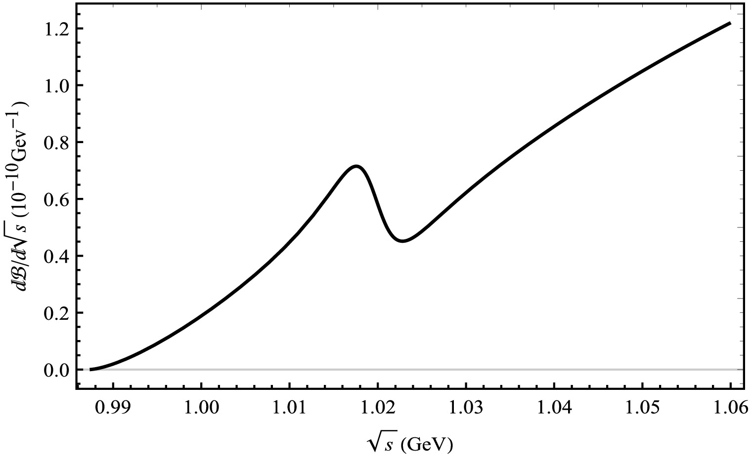
Figure 8. Differential branching ratios for the
$ B_{c}^{+} \rightarrow $ $ D^{+}V \rightarrow D^{+}K^{+}K^{-} $ decay process from the mixing of ϕ, ρ, and ω mesons.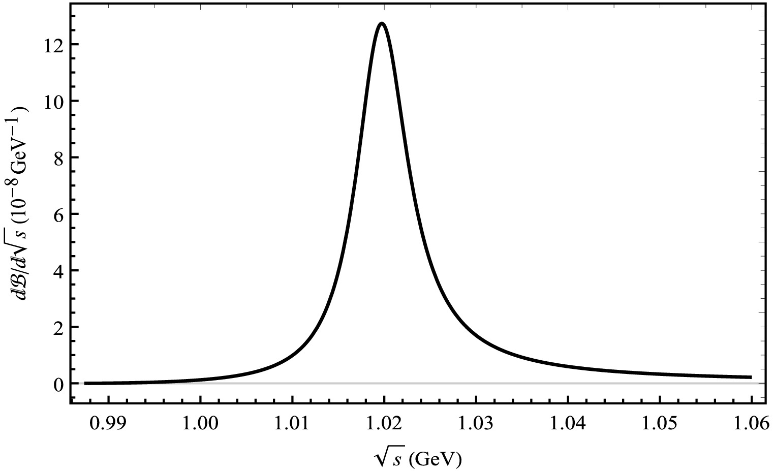
Figure 9. Differential branching ratios for the
$ B_{c}^{+} \rightarrow $ $ D_{s}^{+}V \rightarrow D_{s}^{+}K^{+}K^{-} $ decay process from the mixing of ϕ, ρ, and ω mesons.As illustrated in Figs. 10 and 11, we offer the distribution of the branching ratios of the invariant mass of two π-mesons under the mixed mechanism. In Fig. 10, an obvious peak exists near the mass of the ρ meson. In Fig. 11, a pronounced peak can likewise be discerned near the mass of the ρ meson, while a small peak is present near the mass of the ϕ meson.
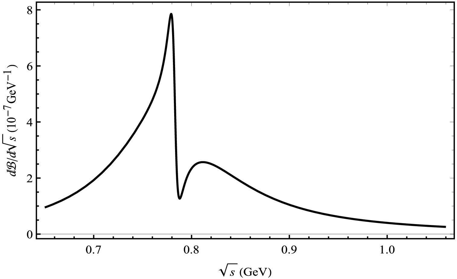
Figure 10. Differential branching ratios for the
$ B_{c}^{+} \rightarrow $ $ D^{+}V \rightarrow D^{+}\pi^{+}\pi^{-} $ decay process from the mixing of ϕ, ρ, and ω mesons.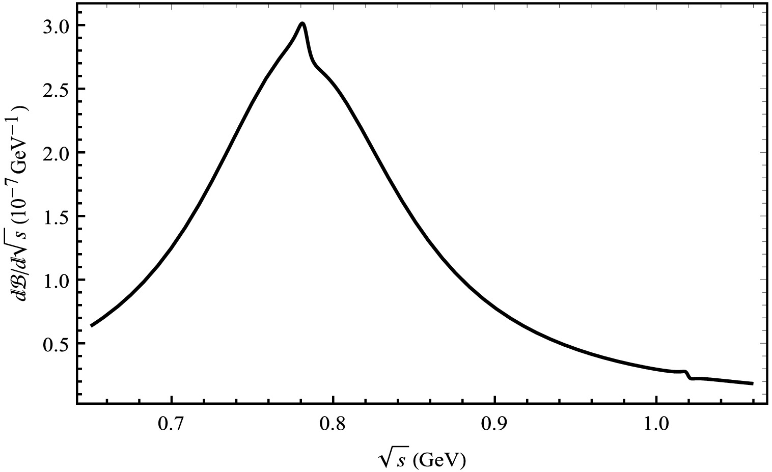
Figure 11. Differential branching ratios for the
$ B_{c}^{+} \rightarrow $ $ D_{s}^{+}V \rightarrow D_{s}^{+}\pi^{+}\pi^{-} $ decay process from the mixing of ϕ, ρ, and ω mesons.Decay channel Branching ratio Direct three-body decay/Mixed three-body decay $ B_{c}^{+} \rightarrow D^{+}\rho^0 \rightarrow D^{+}K^{+}K^{-}$ 

$\mathrm{1.66^{+0.15}_{-0.31}\times10^{-11}}$ 

35.37% $ B_{c}^{+} \rightarrow D^{+}\omega \rightarrow D^{+}K^{+}K^{-}$ 

$\mathrm{2.36^{+0.37 }_{-0.37 }\times10^{-11}} $ 

50.21% $ B_{c}^{+} \rightarrow D^{+}\phi \rightarrow D^{+}K^{+}K^{-}$ 

$\mathrm{4.37^{+0.20}_{-0.21 }\times10^{-11}} $ 

92.98% $ B_{c}^{+} \rightarrow D^{+}\phi (\rho^0,\omega) \rightarrow D^{+}K^{+}K^{-}$ 

$\mathrm{4.70^{+0.53}_{-0.51 }\times10^{-11}} $ 

1 $ B_{c}^{+} \rightarrow D_s^{+}\rho^0 \rightarrow D_s^{+}K^{+}K^{-}$ 

$ \mathrm{1.10^{+0.15}_{-0.14 }\times10^{-11}}$ 

0.0083% $ B_{c}^{+} \rightarrow D_s^{+}\omega \rightarrow D_s^{+}K^{+}K^{-}$ 

$ \mathrm{3.76^{+0.48}_{-0.47 }\times10^{-12}}$ 

0.0028% $ B_{c}^{+} \rightarrow D_s^{+}\phi \rightarrow D_s^{+}K^{+}K^{-}$ 

$ \mathrm{1.44^{+0.95}_{-0.24 }\times10^{-7}}$ 

109.09% $ B_{c}^{+} \rightarrow D_s^{+}\phi (\rho^0,\omega) \rightarrow D_s^{+}K^{+}K^{-}$ 

$ \mathrm{1.32^{+0.12}_{-0.12 }\times10^{-7}}$ 

1 Table 2. PQCD predictions of the branching ratios for quasi-two-body decays
$ B_{c}^{+} \rightarrow D^{+}V \rightarrow D^{+}K^{+}K^{-}$ and$ B_{c}^{+} \rightarrow D_s^{+}V \rightarrow D_s^{+}K^{+}K^{-}$ .The computed local integral values for the decay processes
$ B_{c}^{+} \rightarrow D^{+}V \rightarrow D^{+}\pi^{+}\pi^{-} $ and$ B_{c}^{+} \rightarrow D_{s}^{+}V \rightarrow D_{s}^{+}\pi^{+}\pi^{-} $ are$ 9.037 \times 10^{-7} $ and$ 4.55 \times 10^{-8} $ , respectively. The quasi-two-body decay results are$ 6.61 \times 10^{-7} $ and$ 2.63 \times 10^{-7} $ , respectively. From the outcomes of CP violation presented in Table 3, it can be observed that in the process$ B_{c}^{+} \rightarrow D^{+}\rho^0 \rightarrow D^{+}\pi^{+}\pi^{-} $ , the mixed resonance augments the decay amplitude. Therefore, the branching ratio of the mixed resonance is marginally larger than that of the quasi-two-body decay. However, the mixed resonance in the process$ B_{c}^{+} \rightarrow D_s^{+}\rho^0 \rightarrow D_s^{+}\pi^{+}\pi^{-} $ attenuates the decay amplitude, leading to a branching ratio that is one order of magnitude lower than that of the quasi-two-body decay. We hold the view that the mutual cancellation of the interference terms in the mixed decay process gives rise to a smaller total branching ratio outcome.Decay channel The three-particle admixture in this paper Quasi-two-body $ B_{c}^{+} \rightarrow D^{+}\rho^0 \rightarrow D^{+}\pi^{+}\pi^{-}$ 

$\mathrm{9.037^{+0.30}_{-0.21 }\times10^{-7}} $ 

$\mathrm{6.61^{+1.64}_{-0.99 }\times10^{-7}} $ 

$ B_{c}^{+} \rightarrow D_s^{+}\rho^0 \rightarrow D^{+}\pi^{+}\pi^{-}$ 

$\mathrm{4.55^{+0.33}_{-0.31 }\times10^{-8}} $ 

$\mathrm{2.63^{+0.35}_{-0.35 }\times10^{-7}} $ 

Table 3. Vranching ratio results of
$ B_{c}^{+} \rightarrow D^{+}V \rightarrow D^{+}\pi^{+}\pi^{-}$ and$ B_{c}^{+} \rightarrow D_s^{+}V \rightarrow D_s^{+}\pi^{+}\pi^{-}$ .We also present the outcomes of quasi-two-body decay for comparison.We find that in the decay of
$ B_{c}^{+} \rightarrow D^{+}V \rightarrow D^{+}K^{+}K^{-} $ ,$ D^{+}\phi $ constitutes the dominant contribution, with a branching ratio of$ 92$ %, while the branching ratios of the three direct decay modes$ B_{c}^{+} \rightarrow D^{+}\phi\rightarrow D^{+}K^{+}K^{-} $ ,$ B_{c}^{+} \rightarrow D^{+}\rho^0 \rightarrow D^{+}K^{+}K^{-} $ , and$ B_{c}^{+} \rightarrow D^{+}\omega \rightarrow D^{+}K^{+}K^{-} $ are of the same order of magnitude. The absence of tree-level diagrams in the two-body decay of$ B_{c}^{+} \rightarrow D^{+}\phi $ leads to a small branching ratio for$ B_{c}^{+} \rightarrow D^{+}\phi \rightarrow D^{+}K^{+}K^{-} $ . Meanwhile, the sum of the branching ratios of the three direct decays is significantly larger than the branching ratio of the mixed decay, which can be attributed to destructive interference.In the decay of
$ B_{c}^{+} \rightarrow D_s^{+}V \rightarrow D_s^{+}K^{+}K^{-} $ , the branching ratio of$ B_{c}^{+} \rightarrow D_s^{+}\phi \rightarrow D_s^{+}K^{+}K^{-} $ constitutes$ 109$ % of the branching ratio of the mixed decay. The branching ratios of the other two direct decays are four or five orders of magnitude lower than that of the mixed decay and are therefore negligible. The fact that the branching ratio of$ B_{c}^{+} \rightarrow D_s^{+}\phi \rightarrow D_s^{+}K^{+}K^{-} $ exceeds that of the mixed decay is also attributed to destructive interference. -
The CP violation in the decay process of
$ B_{c}^{+} $ meson is predicted through an invariant mass analysis of$ \pi^+\pi^- $ and$ K^{+} K^{-} $ meson pairs within the resonance region, resulting from the mixing of ϕ, ω, and$ \rho^0 $ mesons. We observe a sharp change in CP violation within the resonance regions of these mesons. Local CP violation is quantified by integrating over phase space. For the decay processes$ \ B_{c}^{+} \rightarrow D^{+}\pi^{+}\pi^{-} $ and$ B_{c}^{+} \rightarrow D^{+}K^{+}K^{-} $ , the CP violation changes significantly from the effects of$ \rho^0 -\omega-\phi $ mixing in the ranges of resonance. Experimental detection of local CP violation can be achieved by reconstructing the resonant states of ϕ, ω, and$ \rho^0 $ mesons within the resonance regions.Our calculation results for the branching ratios indicate that the combined branching ratios of the three direct decays exceed those of the mixed decays in the processes
$ B_{c}^{+} \rightarrow D^{+}\phi (\rho^0,\omega) \rightarrow D^{+}K^{+}K^{-} $ and$ B_{c}^{+} \rightarrow D_s^{+}\phi (\rho^0,\omega) \rightarrow D_s^{+}K^{+}K^{-} $ . The contributions from the three direct decays, along with additional interference terms, influence the overall branching ratio, especially for the decay process of$ B_{c}^{+} \rightarrow D^{+}\phi (\rho^0,\omega) \rightarrow D^{+}K^{+}K^{-} $ . Meanwhile, we computed the branching ratio of process$ B_{c}^{+} \rightarrow D_{(s)}^{+}V \rightarrow D_{(s)}^{+}\pi^{+}\pi^{-} $ and conducted a systematic comparative analysis and in-depth discussion with the research findings of the quasi-two-body decay approach. The outcomes manifested the influence of the mixed resonance. -
The
$ V_{t b} $ ,$ V_{t s} $ ,$ V_{u b} $ ,$ V_{u s} $ ,$ V_{t d} $ , and$ V_{u d} $ terms in the above equation are derived from the CKM matrix element within the framework of the Standard Model. The CKM matrix, whose elements are determined through experimental observations, can be expressed in terms of the Wolfenstein parameters A, ρ, λ, and η:$ V_{t b} V_{t s}^{*} = \lambda $ ,$ V_{u b} V_{u s}^{*} = A \lambda^{4}(\rho- {\rm i} \eta) $ ,$ V_{u b} V_{u d}^{*} = A \lambda^{3}(\rho- {\rm i} \eta)(1-\frac{\lambda^{2}}{2}) $ , and$ V_{t b} V_{t d}^{*} = A \lambda^{3}(1- \rho+ {\rm i} \eta) $ . The most recent values for the parameters in the CKM matrix are$ \lambda = 0.22650\pm 0.00048 $ ,$ A = 0.790_{-0.012}^{+0.017} $ ,$ \bar{\rho} = 0.141_{-0.017}^{+0.016} $ , and$ \bar{\eta} = 0.357\pm 0.011 $ . Here, we define$ \bar{\rho} = \rho\left(1-\dfrac{\lambda^{2}}{2}\right) $ and$ \bar{\eta} = \eta\left(1-\dfrac{\lambda^{2}}{2}\right) $ [37, 38]. The physical quantities involved in the calculation are presented in Table A1.$ m_{B_{c}} = {6.27447}\pm0.27 $ 

$ f_{\phi} = {0.231} $ 

$ m_{D_{s}^+} = {1.96835}\pm0.07 $ 

$ f_{k} = {0.160} $ 

$ m_{K^{\pm}} = {0.493677}\pm0.013 $ 

$ f_{\phi}^{T} = {0.200} $ 

$ m_{W} = {80.3692}\pm0.0133 $ 

$ f_{\rho} = {0.209} $ 

$ m_{\phi} = {1.019431}\pm0.016 $ 

$ f_{\pi} = {0.131} $ 

$ m_{\pi^\pm} = {0.13957}\pm0.00017 $ 

$ f_{\rho}^{T} = {0.165} $ 

$ m_{\omega} = {0.78266}\pm0.13 $ 

$ f_{D} = {0.2067}\pm0.0089 $ 

$ \Gamma_{\rho} = {0.15} $ 

$ f_{B_{c}} = {0.489} $ 

$ m_{\rho} = {0.77526}\pm0.23 $ 

$ f_{D_{s}} = {0.2575}\pm0.0061 $ 

$ \Gamma_{\omega} = {8.49e-3} $ 

$C_F$ = 4/3

$ m_{D^+} = {1.86966}\pm0.05 $ 

$ f_{\omega}^{T} = {0.145} $ 

$ \Gamma_{\phi} = {4.23e-3} $ 

$ f_{\omega} = {0.195} $ 

CP violations and branching ratios for Bc+→ D(s)+π+π−(K+K−) from interference of the vector mesons in Perturbative QCD
- Received Date: 2025-03-02
- Available Online: 2025-09-15
Abstract: Within the framework of the perturbative QCD approach utilizing


 DownLoad: