Nonlinear diffusive shock acceleration with upstream escape reproduces DAMPE observations

Diffusive shock acceleration (DSA) is widely regarded as the primary mechanism for accelerating cosmic rays (CRs) in astrophysical systems [1−4]. In the standard test-particle scenario, particles are assumed to gain energy only upon crossing the shock front, corresponding microscopically to first-order Fermi acceleration. Each shock crossing imparts a momentum gain proportional to the velocity difference across the shock, while there is a finite probability that particles are advected downstream and thus lost from the acceleration region, resulting in the well-known power-law spectrum. A central assumption of the test-particle limit is that the accelerated particles exert no influence on the background plasma, that is, there is no feedback.

Building on earlier work [5−7], Malkov et al. [8, 9] demonstrated that non-thermal particles accelerated by the shock can modify the shock structure, particularly in the upstream region. This feedback can induce a continuous velocity gradient in the upstream fluid due to the CR pressure gradient, forming a precursor. Within such a structure, particles can undergo acceleration throughout their upstream propagation, rather than solely at the shock front. Because the diffusive-advective propagation distance of CRs scales as $ D/u $, where D is the spatial diffusion coefficient and u is the bulk-flow speed, higher-energy particles can penetrate farther upstream before returning to the shock. Consequently, higher-energy particles experience a larger velocity gradient in the background flow and receive greater acceleration, leading to spectral hardening at the high-energy end—manifested as an energy-dependent deviation from a single power-law spectrum.

In Malkov’s formulation, closure of the nonlinear system is achieved by imposing a sharp upper momentum cutoff $ p_1 $, beyond which the CR distribution is abruptly truncated. While mathematically convenient, this assumption departs from the more physically motivated expectation of a gradual exponential cutoff (e-cut) that typically depends on the atomic number Z and arises from finite acceleration timescales or from escape through an upstream boundary. Moreover, key quantities such as the precursor compression ratio are determined by a mechanism of self-organized criticality that is intrinsically linked to the presence of this hard cutoff.

In this work, we improve upon Malkov’s approach in two key aspects. First, rather than imposing an ad hoc sharp cutoff at $ p_1 $, we model the high-energy termination of the CR spectrum using a physically motivated exponential cutoff that naturally emerges from upstream escape, an unavoidable feature of realistic acceleration sites. Second, the precursor compression ratio is determined self-consistently from physically motivated boundary conditions, instead of being fixed by an externally imposed closure prescription. Within our framework, CR heating introduces a stabilizing negative feedback that regulates the nonlinear response of the system, contributes to downstream plasma heating, and ensures the existence of a well-behaved solution. By treating the upstream region as a constrained system bounded by the downstream thermal reservoir and the far-upstream medium, and by enforcing consistent injection conditions across the shock, the precursor compression ratio is implicitly fixed by the requirement that all physical boundary conditions be satisfied simultaneously.

Recent observations from DAMPE reveal a Z-dependent e-cut, accompanied by gradual spectral hardening from tens of GeV to several TeV before the cutoff. Several mechanisms could, in principle, produce spectra with both hardening and an exponential cutoff, including reacceleration by a local shock [10, 11], superposition of multiple source components [12, 13], and self-consistent halo models [14].

Motivated by these observations, we develop a feedback-driven acceleration model that self-consistently incorporates an e-cut through upstream escape. Our numerical calculations show that this model can reproduce the latest DAMPE proton spectrum [15] under conventional single-zone diffusion propagation in the Galaxy, thereby providing a physically motivated explanation for the observed spectral hardening followed by a cutoff.

This paper is organized as follows: Section II outlines the methodology; Section III presents a comparison between the model predictions and DAMPE observations and discusses the physical interpretation of the results; and Section IV summarizes the main results.

Consider a planar shock propagating in the positive x-direction. In the shock rest frame, the upstream region is at $ x>0 $, the downstream region at $ x<0 $, and the shock front is located at $ x=0 $. The phase-space distribution of CR particles is denoted by $ f(x,p) $. The bulk plasma velocity in this frame is $ u(x) $, directed opposite to the positive x-direction. Throughout, we normalize momentum by the particle rest mass times c; that is, $p \rightarrow p/(mc)$, unless stated otherwise. The physical momentum is then recovered by multiplying by $mc$. This convention simplifies the integral expressions for the CR pressure in Sec. II B and other momentum-space integrals. Note that, irrespective of this normalization, the operator $p\partial_p$ and the differential $\mathrm{d}p/p$ are dimensionless.

In this coordinate system, the original DSA transport equation for the phase-space distribution $f(x,p)$ is

Time-dependent numerical solutions of related DSA equations can, in principle, be obtained, for example, using SDE-based methods [16]. In the present work, however, we consider only the stationary problem, namely, $\partial_t f=0$ in Eq. (1).

It is convenient to reformulate the problem in terms of the function $ g(x,p)\equiv p^{3}f(x,p) $. With this definition, $ g(x,p) $ can be interpreted as the CR number density per logarithmic momentum interval, $ \mathrm{d}N/\mathrm{d}\ln p = 4\pi g $. In the stationary case, with this convention for g, Eq. (1) can be recast as follows [8]:

where

Here, $ J(x,p) $ denotes the combined convective and diffusive particle flux, expressed in terms of $ g(x,p) $, with the natural upstream boundary condition $ J(\infty,p)=0 $. By convention, this flux has the opposite sign to the actual net particle flux in the upstream region. The right-hand side of Eq. (2) describes particle acceleration due to compression of the background flow. Throughout this work we assume a spatially homogeneous diffusion coefficient $ D(p) $ that depends only on momentum.

In the test-particle limit, the convection-velocity gradient is confined to the shock front and can be written as $ \mathrm{d}u/\mathrm{d}x = \Delta u\,\delta(x), $ where $\Delta u \equiv u_{0}-u_{2}$ denotes the velocity jump across the shock. Here, $u_{0}$ is the convection velocity immediately upstream of the shock at $x=0^{+}$; in the test-particle approximation, it coincides with the constant flow velocity throughout the entire upstream region. The downstream flow velocity $u_{2}$ is likewise taken to be constant throughout the downstream region.

Because the downstream region is sufficiently extended and contains an abundant population of thermal particles, the convective and diffusive fluxes there are aligned, which prevents the buildup of a CR density gradient. Consequently, the downstream solution equals the distribution at the shock front, $ g(x <0,p)= g_{0}(p)\equiv g(0^{+},p)=g(0^{-},p). $

We define the function

which represents the integrated flow-velocity profile.

With these considerations, the upstream distribution can be obtained by combining Eq. (2) and Eq. (3) as

At this stage, it is convenient to introduce the Green's function $ G(x,x',p) $, defined by

The solution can be rewritten in compact form as

Under the test-particle approximation, the integral term in Eq. (7) vanishes; consequently, the upstream distribution simplifies to

To determine the momentum dependence at the shock, we integrate Eq. (2) across a narrow interval containing the shock front to obtain the equation governing $ g_{0}(p) $:

Substituting the upstream solution for $ g(x,p) $ from Eq. (8) into Eq. (9) yields

This equation expresses the balance between the flux of particles advected downstream to infinity and the momentum gain due to compression at the shock front. Its solution is a power-law spectrum.

where $ r_{s}\equiv u_{0}/u_{2} $ is the shock compression ratio and $ p_{\mathrm{inj}} $ denotes the injection momentum. The corresponding spectral index of the phase-space distribution $ f_{0}(p) $ is given by the well-known expression $ -3r_{s}/(r_{s}-1) $.

In the test-particle regime of diffusive shock acceleration, the upstream region is effectively infinite, so that convection always returns particles to the shock, regardless of their energy, yielding a spectrum without a high-energy cutoff. In realistic acceleration environments, however, the upstream region has a finite spatial extent, and particle transport is governed by the competition between diffusion and convection. Once a particle’s diffusion length exceeds the characteristic size of the system, it is likely to escape upstream before being advected back to the shock. As we show below, this escape process naturally leads to an exponential cutoff (e-cut) in the energy spectrum. Two complementary approaches are commonly employed to model such finite-system effects:

1. Absorbing-boundary model: A physical absorbing boundary is imposed at a fixed upstream distance L. Particles reaching $ x=L $ are instantaneously removed from the system, thereby establishing an explicit maximum diffusion scale [17, 18].

2. Escape-term model: A momentum-dependent escape term, $ -f/\tau_{\mathrm{esc}} $, is introduced into the transport equation. The escape rate $ \tau_{\mathrm{esc}}^{-1}=D/\xi^{2} $ encapsulates the idea that particles with larger diffusion coefficients (corresponding to higher momenta) escape more efficiently from a region of characteristic size ξ. This formulation directly captures the competition between diffusion and escape processes [19−22].

In this work, we adopt the latter approach; accordingly, Eq. (2) is modified to:

while the corresponding solution for $ g(x,p) $, obtained by replacing Eq. (7), reads

In the test-particle limit, the solution to Eq. (13) has the form $ g(x,p)=g_{0}(p)\,e^{-k(p)x} $, where $ k>0 $. Substituting this ansatz into Eq. (13) yields the condition that k must satisfy:

which admits the solution

Here, $v_{\mathrm{esc}}(p)\equiv D/\xi$ can be interpreted as an effective escape velocity associated with diffusive transport.

Substituting this result into Eq. (9), one obtains the particle spectrum at the shock:

It follows that when $ v_{\mathrm{esc}}\sim u_{0} $, escape becomes significant, and the spectrum begins to deviate from a pure power law. In the high-energy limit, $v_{\mathrm{esc}}\gg u_{0}$, the integrand appearing in the exponential scales approximately as $v_{\mathrm{esc}}/u_{0}$, leading to a pronounced exponential cutoff in the spectrum.

In the presence of CR acceleration, the upstream diffusion–convection balance produces a CR pressure gradient that, in turn, drives a spatial gradient in the background flow, so that the upstream velocity $ u(x) $ becomes position-dependent. Starting from Eq. (12) and following the procedure leading to Eq. (7), the upstream distribution $ g(x,p) $ satisfies:

The functional $ W[g] $ accounts for compression and particle escape and is defined by:

The source term $ S[g](x,p) $ accounts for both acceleration and particle escape effects.

Here, the acceleration term depends on the velocity-gradient distribution throughout the upstream precursor, which is self-consistently driven by cosmic rays; therefore, acceleration occurs not only at the shock front but also across the entire upstream region.

To proceed, we treat Eq. (17) perturbatively about the homogeneous solution. The zeroth-order solution, $ g^{(0)}(x,p) $, corresponds to pure advection–diffusion in the absence of sources and is given by

Equation (20) follows from the homogeneous part of Eq. (17), obtained by setting $S[g]=0$, assuming that D depends only on momentum, and by imposing the boundary condition $g(0,p)=g_0(p)$. For later convenience, we define the shock spectral index as $q(p)\equiv -\partial\ln f_{0}/\partial\ln p = 3-\partial\ln g_{0}/\partial\ln p$.

We then evaluate the first-order correction by substituting $g^{(0)}$ into $W[g]$. In the main support region of $g^{(0)}$, where $xu/D \ll 1$ and $v_{\mathrm{esc}}/u \ll 1$, the correction remains perturbative, and the approximation $g^{(1)} = g^{(0)} + W[g^{(0)}] = g^{(0)} \left(1+W[g^{(0)}]/g^{(0)}\right) \simeq g^{(0)}e^{W[g^{(0)}]/g^{(0)}}$ is well justified [8]. We therefore obtain

Here, higher-order terms proportional to $D^{-1}$ have been neglected.

Since $ q/3>1 \gg (v_{\mathrm{esc}}/u)^{2} $, the upstream distribution may be approximated as

For computational simplicity, we omit higher-order corrections associated with the truncation. As discussed in Appendix A, such corrections tend to reduce the feedback strength of the pre-truncation system. Nevertheless, numerical studies by Caprioli [23], based on a related but distinct nonlinear model, indicate that accounting for higher-order truncation effects in the feedback does not substantially alter the spectral shape below the cutoff. Rather, the dominant impact of truncation is confined to the high-energy region beyond the cutoff.

With the inclusion of escape and feedback effects, Eq. (9) is modified to

Using the first-order approximation $ g^{(1)} $, the combined effects of escape and nonlinear feedback can be formulated as a closed equation for the momentum-dependent spectral index $ q(p) $.

Here, the subscript $ 1 $ denotes quantities evaluated at the far-upstream boundary. $ R\equiv u_{1}/u_{0} $ is the compression ratio across the entire upstream precursor, while $ Rr_{s}=u_{1}/u_{2} $ is the total compression ratio of the system. The parameter $ \alpha\equiv\bar{u}/u_{1}\in[R^{-1},1] $ characterizes the effective upstream flow speed sampled by the particles. To quantify particle escape, we introduce a cutoff parameter χ, defined at the reference momentum $ p=1 $ (in units of mc), as

A larger value of χ delays the onset of the exponential cutoff. Assuming that the diffusion coefficient follows a power law, $ D(p)\propto p^{\beta} $, we can rewrite the escape term and $ q(p) $ in terms of χ:

Once $q(p)$ has been obtained, we use it to compute $ g_{0}(p) $:

The cumulative normalized velocity gradient experienced by particles with momentum p is defined as

where $ V(p) $ denotes the weighted contribution of the spatially distributed velocity gradient.

To obtain the spectral index $ q(p) $, we require the flow-velocity gradient $\mathrm{d}u/\mathrm{d}x$ to compute $ V(p) $. The flow-field distribution is then self-consistently driven by CR pressure, following the standard mass and momentum conservation equations [24]:

where $ P_g $ denotes the thermal pressure. The CR pressure is given by

v denotes the particle velocity in the laboratory frame, and we use relativistic kinematics for convenience. It is useful to separate the overall normalization from the momentum-dependent shape by writing

with $\tilde{g}(x,p)$ normalized so that $\tilde{g}(0,p_{\mathrm{inj}})=1$. The quantity $g_{0}(p_{\mathrm{inj}})$ is the shock-frame distribution function at the injection momentum; it has units of number density. The combination $\dfrac{4\pi}{3} m c^2 g_0(p_{\mathrm{inj}})$ therefore has units of pressure and sets a characteristic scale for the CR pressure contributed by the injected particles. Physically, it corresponds to the CR pressure that would obtain if all injected particles were concentrated at the injection momentum, with a phase-space density $f_0(p_{\mathrm{inj}})$, and treated in the relativistic limit (where $p \gg mc$). In practice, the full CR pressure is obtained by integrating over the entire momentum distribution; it scales linearly with this characteristic pressure, with the proportionality factor set by the spectral shape. Motivated by this, we introduce a dimensionless injection-rate parameter:

This parameter quantifies the ratio of the characteristic CR pressure to the incoming ram pressure $\rho_1 u_1^2$. Physically, η directly controls the strength of nonlinear feedback: the CR pressure scales as $P_{\mathrm{CR}} \propto \eta \times (\rho_1 u_1^2)$. More explicitly, using the definition of η and the normalized distribution $\tilde{g}$, the CR pressure at any position x can be written as

This shows that η sets the overall normalization of the CR pressure relative to the ram pressure. If no particles are injected, $\eta = 0$ and consequently $g_{0}(p_{\mathrm{inj}})=0$. Then Eq. (35) gives $P_{\mathrm{CR}}(x)=0$ everywhere. In that case, the momentum conservation equation, Eq. (31), reduces to $\rho u^{2}+P_{g}= \rho_{1}u_{1}^{2}+P_{g,1}$. Together with the adiabatic relation $P_{g}\propto \rho^{\gamma}$ and the mass conservation equation, Eq. (30), this algebraic relation implies $u(x)=u_{1}$ for all x; the upstream flow remains unperturbed and no feedback operates.

In the presence of injection ($\eta>0$), the CR pressure modifies the flow. To proceed, we neglect the thermal pressure $P_{g}$ in the momentum balance when evaluating the velocity gradient. This leading-order approximation is justified in the strong-shock regime, in which the ram pressure dominates and the CR pressure provides the main correction to the upstream flow [1, 2, 8]. Using Eqs. (30) and (31), together with (33), we obtain an expression for $\mathrm{d}u/\mathrm{d}x$ that depends on the CR distribution. Substituting this into the definition of $V(p)$, Eq. (29), and employing the first-order approximation for $g(x,p)$, Eq. (22), yields

which can be evaluated analytically to yield

Equation (37) explicitly shows that the cumulative velocity-gradient measure $V(p)$ is proportional to the injection rate η. Thus, η serves as the strength parameter of the nonlinear feedback: a larger η implies that more particles are injected, leading to stronger CR pressure and a more pronounced modification of the upstream flow. In the limit $\eta\to0$, $V(p)\to0$, and the system reverts to the test-particle description with no spectral hardening. This linear scaling of V with η further implies that the shock’s entire nonlinear response is governed by the single dimensionless parameter η, which is itself set by the microphysics of injection, as described in Sec. II C.

The acceleration framework introduced in Section II B is characterized by a set of key parameters summarized in Table 1. These include the precursor compression ratio R, the subshock compression ratio $r_s$, the injection rate η, the injection momentum $p_{\text{inj}}$, the diffusion coefficient $D(p)$, and the far-upstream Mach number $M \equiv u_1 / c_{s,1}$. Most of these quantities are not free parameters; rather, they are constrained by boundary conditions and fundamental physical relations.

In general, particles injected into the acceleration process originate from the high-energy tail of the downstream thermal distribution, where their momenta exceed the thermal momentum by factors of a few [25, 26]. Only these suprathermal particles have a non-negligible probability of recrossing the shock and entering the diffusive acceleration cycle. The injection momentum is therefore parametrized as $p_{\text{inj}} = \zeta p_{\text{th},2}$, where the dimensionless parameter ζ (typically in the range $2 - 4$; see, e.g., [25, 26]) sets the injection threshold in units of the downstream thermal momentum $p_{\text{th},2}$. This yields

where the far-upstream thermal momentum is defined as $p_{\text{th},1} = \sqrt{2 m k_B T_1}$. The temperature jump $T_2/T_0$ across the subshock is determined by the Rankine–Hugoniot relations, and upstream compression yields

Under purely adiabatic compression, the thermal gas pressure follows $P_g \propto \rho^{\gamma}$, where γ is the adiabatic index of the background plasma. In the non-adiabatic case, however, additional heating results from CR-induced wave excitation in the precursor. The heating due to wave energy can be described by the first law of thermodynamics [6, 26].

which, upon combining Eqs. (30) and (31), can be recast as

Here, $v_s$ denotes the speed of backward-propagating waves excited in the upstream medium, with $v_s \propto u^{s}$; the choice $s=1/2$, which typically corresponds to Alfvén-wave heating, is adopted as the default in this work.

The resulting gas pressure profile in the precursor can then be written as

where the nonadiabatic correction factor is given by

where $M_s \equiv u_1 / v_{s,1}$. In the limit $M_s \to \infty$, the correction term vanishes ($H \to 0$), recovering the adiabatic result.

With these ingredients, the injection momentum can be expressed as

where $H_0 \equiv H(x=0)$. The subshock compression ratio $r_s$ is obtained from momentum conservation and the Rankine–Hugoniot conditions, yielding:

As discussed in Section II B, the injection rate η controls the strength of the nonlinear feedback in the system. Physically, η characterizes the leakage of particles from the downstream thermal pool into the non-thermal population. Starting from Eq. (34), we model the downstream thermal population with a Maxwellian distribution:

with the downstream number density $n_2 = R r_s n_1$. We then impose the injection matching condition $f_0(p_{\mathrm{inj}})= f_{\mathrm{th},2}(p_{\mathrm{inj}})$. A similar matching prescription has also been employed in numerical studies of shock injection; see, e.g., [27]. Since $g_0(p)=p^3 f_0(p)$ and $p_{\mathrm{inj}}=\zeta p_{\mathrm{th},2}$, substituting these relations into Eq. (34) yields

Given ζ, M, and $p_{\text{th},1}$ (or, equivalently, $T_1$), this relation uniquely determines η.

From a complementary perspective, η also quantifies the injection strength required to sustain a precursor compression ratio R in the nonlinear regime. Using Eq. (30)–(31) together with the boundary condition $R = u_0 / u_1$, we obtain

The physically realized value of the precursor compression ratio R is fixed by requiring that the two independent estimates of the injection rate coincide. Equivalently, Eq. (48) must equal Eq. (47), thereby ensuring consistency between the microphysical injection process and the global, nonlinear modification of the shock.

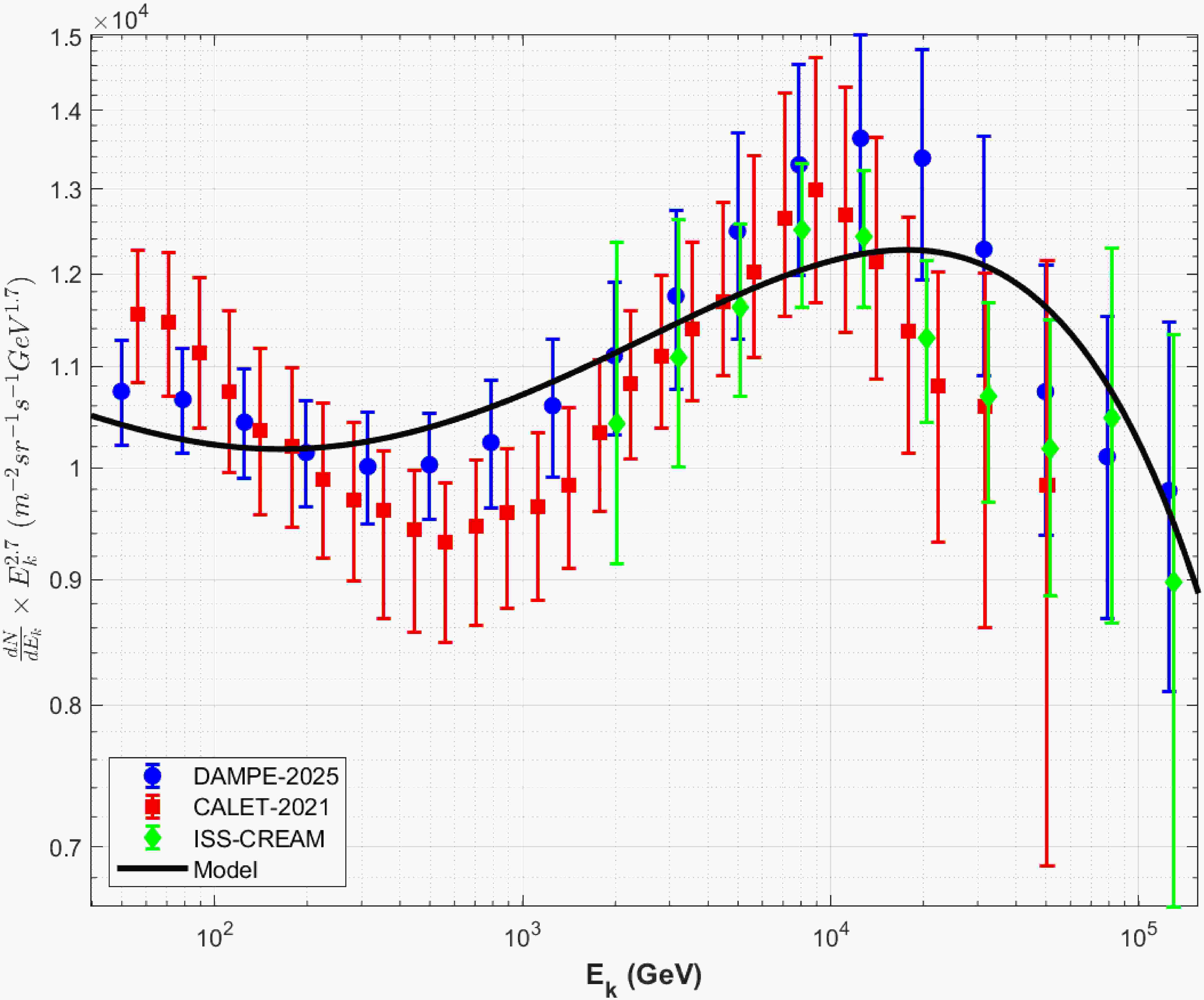
To enable direct comparison with DAMPE observations, the source spectrum must be consistently linked to the propagated spectrum at Earth. Within the conventional one-zone diffusion–propagation framework, the observed differential flux as a function of kinetic energy is given by

where the prefactor $ (E_{\text{k}} + m_p c^2) $ arises from the transformation between momentum and kinetic-energy spaces, and $ m_p $ denotes the proton mass. In addition, we revert to using momentum with physical dimensions. The second factor accounts for CR propagation in the interstellar medium, which we approximate as a softening of the source power-law index by a factor $ p^{-\delta} $. The diffusion coefficient is parameterized as $ D_{\text{ISM}} \propto p^{\delta} $, with $ \delta = 0.5 $ fixed by fits to the boron-to-carbon (B/C) ratio, consistent with previous studies [28−31]. The final factor, $ \tilde{g}_0 $, represents the injected source spectrum computed from Eq. (27). This assumes that the observed CRs are the particles accumulated downstream during the active acceleration phase and released when the shock wave dissipates. For the comparison in Fig. 2, we fix the overall normalization of the theoretical curve by setting its value at $E_{\text{k}} = 100\,\mathrm{GeV}$.

Figure 2.  (color online) Comparison of the theoretical model (black curve) with the latest DAMPE-2025 [15] proton spectrum, as well as the CALET-2022 [32] and ISS-CREAM [33] data.

The self-consistent determination of the precursor compression ratio R is illustrated in Fig. 1. Within the precursor, a larger R corresponds to stronger nonlinear feedback from CRs, implying enhanced shock modification and, consequently, requiring a higher injection rate to sustain the system. This behavior is captured by the blue curve in Fig. 1, which represents the nonlinear response $ \eta(R) $. Independently, the injection rate inferred from thermal leakage (red curve) provides a second constraint. The physically admissible solution is given by the intersection of these two curves, yielding a unique R for a given set of parameters.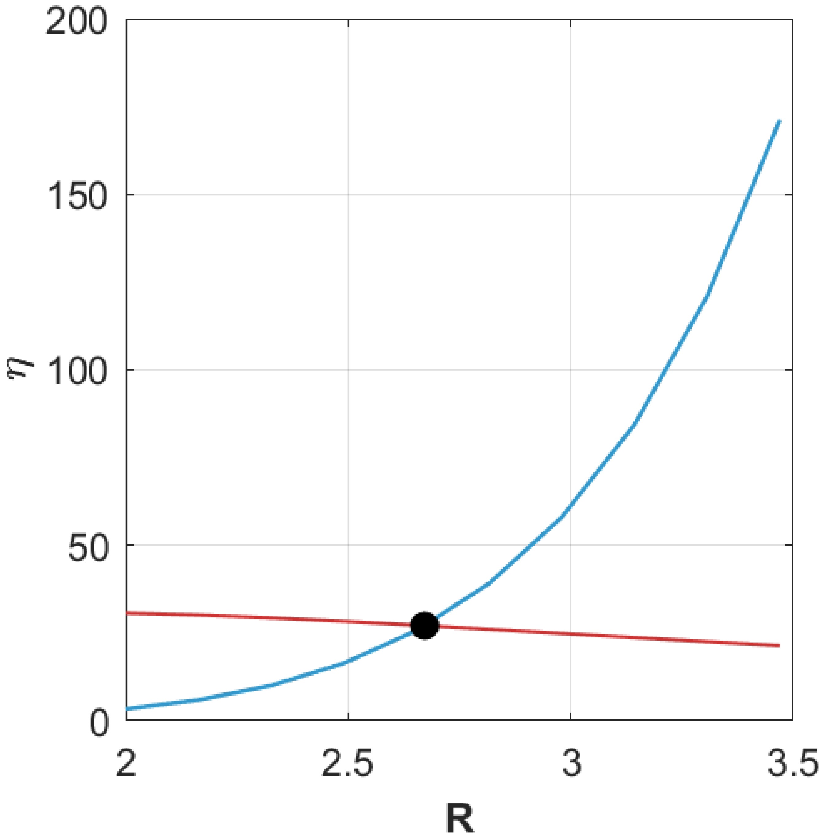

Figure 1.  (color online) Injection-rate response curves for the thermal-injection constraint (red; Eq. (47)) and the system's self-consistent nonlinear response, $ \eta(R) $ (blue; Eq. (48)); their intersection determines the precursor compression ratio R.

An important feature of the nonlinear response curve is the appearance of a distorted (oscillatory) region at intermediate values of R. This distortion arises from the delicate balance between positive feedback from particle injection and negative feedback from plasma heating induced by CR-excited waves. The positive feedback—controlled by the injection parameter ζ—tends to increase R by enhancing the CR pressure gradient, while the negative feedback—governed by the wave-heating parameter $ M_s $—suppresses R by raising the upstream gas pressure and reducing compressibility. When these two effects are not properly matched, the $ \eta(R) $ curve can develop unphysical oscillations or may even fail to intersect the thermal-injection curve, leading to multiple solutions or none at all. In practice, avoiding such pathological behavior requires a balanced pairing: relatively strong injection (small ζ) must be accompanied by strong heating (small $ M_s $), and vice versa. This matching condition ensures that the system remains in a stable, physically realizable regime in which the two curves intersect at a reasonable R, typically within the range $ 2 \lesssim R \lesssim 5 $.

With the above insights, we now apply the model to interpret the latest DAMPE proton spectrum. Adopting parameters characteristic of an early-phase supernova-remnant environment with a strong shock ($ M = 200 $) and a relatively warm upstream medium ($ p_{\mathrm{th},1} = 0.0005\,m_p c $, corresponding to $ T_1 \sim 10^6\,\mathrm{K} $), we fix the diffusion coefficient in the source region to follow $ D(p) \propto p^{1/3} $, consistent with Kolmogorov scaling [34]. The injection parameter $ \zeta = 2.3 $, the wave-heating parameter $ M_s = 14 $, and the cutoff parameter $ \chi \approx 43 $ (defined in Eq. (25)) are chosen such that the thermal-injection and nonlinear-response curves intersect cleanly, yielding a precursor compression ratio $ R \approx 2.7 $ and a subshock compression ratio $ r_s \approx 1.685 $. The resulting source spectrum, after propagation through the Galaxy with the standard diffusion index $ \delta = 0.5 $, is shown in Fig. 2 (black curve) alongside the latest DAMPE data and other measurements. This comparison is intended to illustrate the main spectral features rather than to provide a precision fit to the data. We also tested the case $\delta = 1/3$, which requires a slightly softer injected source spectrum. With $\zeta = 2.1$, $M_s = 11$, and $\chi \approx 47$, the propagated spectrum differs only slightly from the black curve shown in Fig. 2. The model successfully reproduces the gradual hardening from several hundred GeV to multi-TeV energies and the subsequent exponential cutoff above $ \sim 20 $ TeV, with a change in spectral index $ \Delta q \sim 0.2 $.

The slight mismatch at the lowest energies—the predicted onset of hardening appears about $ 100 $ GeV lower than indicated by the data—may be attributed to the neglect of thermal pressure in the calculation of the velocity gradient $ V(p) $, as discussed in Sec. II B. This simplification tends to overestimate $ \mathrm{d}u/\mathrm{d}x $ in the precursor, thereby shifting the hardening to slightly lower energies, but it does not alter the essential physics.

In this model, $U(p)$ encodes the spectral information more directly than $u(x)$. Therefore, to understand the spectral shape in Fig. 2, it is convenient to examine Fig. 3, which shows the energy dependence of the cumulative normalized velocity gradient U and the spectral index q. In the feedback-dominated region below $ \sim 10^{4} $ GeV, a clear anticorrelation between U and q is evident. This arises because higher-energy particles, having larger diffusion coefficients, propagate farther upstream and experience a greater integrated velocity gradient $ V(p) $, as described by Eqs. (28) and (37). Consequently, U increases with energy; via Eq. (26), the spectral index q correspondingly decreases, leading to the gradual hardening of the propagated spectrum.

Figure 3.  (color online) The cumulative normalized velocity gradient U (blue) and the spectral index q (red) are plotted as functions of kinetic energy using the same parameters as in Fig. 2.

A transition occurs around $ 10^{4} $ GeV, beyond which escape effects dominate. At these energies, particles escape from the upstream region before returning to the shock, halting further accumulation of the velocity gradient. As a result, U saturates at an asymptotic value, while the spectral index q increases sharply due to the escape term in Eq. (26), thereby producing the exponential cutoff in the spectrum. This competition between feedback-driven hardening and escape-induced softening naturally accounts for the observed spectral shape.

In this work, we develop and investigate a self-consistent, nonlinear model of diffusive shock acceleration that explicitly incorporates cosmic-ray (CR) feedback and particle escape. Going beyond the standard test-particle framework, we extend the approach of Malkov et al. by introducing two key improvements. First, we implement a physically motivated exponential cutoff (e-cut) in the momentum spectrum that arises naturally from finite upstream boundaries or particle escape, rather than adopting an ad hoc sharp truncation. Second, we determine the precursor compression ratio self-consistently by matching the injection rate inferred from thermal leakage to the nonlinear response required by the system. Within this framework, cosmic-ray-induced wave heating emerges as an essential negative feedback mechanism that counterbalances the positive feedback from particle injection, stabilizes the shock structure, and ensures the existence of physically admissible solutions.

We apply this framework to interpret the latest DAMPE measurements of the CR proton spectrum. Our numerical results show that, within a conventional single-zone diffusion model and for parameters characteristic of young supernova remnants (SNRs), this framework successfully reproduces the observed gradual spectral hardening from hundreds of GeV to several TeV, followed by an exponential cutoff at higher energies. The resulting spectral shape arises naturally from the energy-dependent coupling of particle transport to the shock structure modified by CR pressure in the precursor.

We note that, for numerical tractability, certain higher-order effects are neglected in the present formulation, in particular refinements to particle escape and to the detailed role of thermal pressure near the cutoff. These simplifications may account for minor discrepancies between the model predictions and the data, such as the slightly earlier onset of spectral hardening. A more complete treatment of these effects is deferred to future work.

We now examine, in detail, the effect of escape on nonlinear feedback acceleration. We know that, for the operator

there is a Green's function

satisfying the boundary conditions $G(0, \xi) = G(\infty, \xi) = 0$, where we omit the explicit dependence on p.

Now consider the operator $L_2 = L_1 - \tau_{\text{esc}}^{-1}$ and its Green's function $G_2(x, \xi)$, satisfying:

where $L_{2,x}$ denotes the operator acting on x, we have:

This is equivalent to the following integral equation:

Prior to the cutoff, when $\dfrac{v_{\text{esc}}}{u} \ll 1$, we treat escape as a perturbation and estimate the leading-order behavior:

Now, up to order $D^{-1}$, we estimate:

where

is a first-order approximation to the homogeneous solution of $L_2$, and

From

The above calculation applies when $v_{\text{esc}} \lt u$. Outside this regime, higher-order corrections to $G_2$ must be considered. Nevertheless, the presence of the escape term suppresses the high-energy contribution to $\frac{du}{dx}$ before it suppresses the upstream distribution; that is, it reduces the feedback effect.

A similar behavior is observed with finite boundaries. Set an upstream escape boundary at $x = L$, imposing $g(\xi, p) = 0$. The corresponding Green's function is calculated as:

where the boundary correction factor is

It decreases as momentum increases. At very high energies (beyond the cutoff momentum), it suppresses the system's response approximately linearly.

In the same manner, we have:

and $ g_{0} $ satisfies:

Estimate from Eq. (65):

Consequently, the escape boundary suppresses the contribution of high-energy particles to the feedback on the flow field. Within a region of approximately one diffusion scale $L_{\text{diff}} \sim D/u$ before the escape boundary L, this contribution decays nearly linearly. This suppression becomes significant when $\dfrac{L - L_{\text{diff}}}{L_{\text{diff}}} \lt 1$, roughly corresponding to particles with momenta near the escape momentum at the onset of escape.