


 Abstract
 HTML
HTML Reference
 Related
 PDF
PDF


-
In June 2023, the pulsar timing array (PTA) collaborations NANOGrav [1], EPTA [2], PPTA [3], and CPTA [4] reported evidence for an isotropic, stochastic background of gravitational waves (GWs) within the nanohertz frequency range. The astrophysical origin of the stochastic gravitational-wave background (SGWB) is primarily attributed to supermassive black hole binary (SMBHB) [5, 6]. Furthermore, the PTA observation has provided a new tool for probing new physics [7]. Various sources of the SGWB have been investigated to explain the origin of current PTA observations. The cosmological explanations include cosmic strings and domain walls [8−10], cosmological phase transition GWs [11, 12], and scalar-induced gravitational waves (SIGWs) [13−19]. Afzal et al. [7] has analyzed the possibility that different sources of the SGWB dominate current PTA observations. Their results show that the SIGWs yield the highest Bayes factor, indicating that SIGWs are among the most likely sources of the SGWB in the PTA frequency band.
SIGWs originate from primordial curvature perturbations, with large amplitudes, on small scales. More precisely, based on large-scale cosmological observations, such as cosmic microwave background (CMB) and large-scale structures, the amplitude of the power spectrum corresponding to primordial curvature perturbations is approximately
$ 2\times 10^{-9} $ [20]. However, on small scales ($ \lesssim $ 1 Mpc), current cosmological observations impose significantly weaker constraints on primordial curvature perturbations [21]. Large-amplitude primordial curvature perturbations on small scales can re-enter the horizon after inflation, thereby exciting higher-order SIGWs with significant observable effects. Since the second-order SIGWs are generated by primordial scalar perturbations for a specific inflation model, the parameter space of the inflation model can be constrained by current and future SGWB observations. Over the past two years, the SGWB in the PTA frequency band, dominated by SIGWs, has been systematically studied. Relevant research includes investigations into primordial non-Gaussianity [22−24], varying sound speed [15], different epochs of the Universe [25–27], and corrections from third-order SIGWs [14].In current studies on SIGWs and PTA observations, a statistically isotropic primordial power spectrum on small scales is commonly assumed. This assumption implies that the spectrum
$ {\cal{P}}_{\zeta}(k) $ depends only on the magnitude of the wavenumber$ {\bf{k}} $ , and not on its direction. Given that present PTA data provide evidence for an isotropic SGWB, this assumption of small-scale isotropy appears reasonable. However, notably, this prior assumption is not mandatory. The exploration of the primordial power spectra exhibiting anisotropy on small scales is grounded in strong physical considerations. As indicated in previous studies [28–29], SIGWs originate from extremely high redshifts, corresponding to extremely small horizon scales. Due to the limited angular resolution of current detectors, the signal along any line of sight represents an ensemble average over numerous such horizon patches. Consequently, current PTA observations are incapable of resolving the anisotropy in the primordial power spectra at small scales. Constraining such anisotropic features remains an open question. In this study, we investigate the second-order SIGWs generated by small-scale ($ \lesssim $ 1 Mpc) statistically anisotropic primordial scalar perturbations. Models capable of producing anisotropic primordial perturbations can be primarily categorized into two types: (i) models in which additional fields are introduced during inflation to generate anisotropy at the quantum scale [30−34] and (ii) those incorporating an anisotropic spacetime background, primarily focusing on Finslerian inflation [35−38]. Here, we investigate the impact of anisotropic primordial power spectra on SIGWs using a model-independent approach, specifically a parametric method. When the primordial power spectrum exhibits anisotropy on small scales, the energy density spectra of second-order SIGWs are also anisotropic on small scales. Because the small-scale anisotropy of SIGWs cannot be observed by current PTAs, we derive the isotropic energy density spectrum of SIGWs by spatially averaging the anisotropic SIGWs on small scales. Evidently, the spatial averaging does not eliminate the influence of the anisotropic parameters. The potential small-scale anisotropic primordial power spectra can be constrained by current PTA observations of the isotropic energy density spectrum of SIGWs.The remainder of this paper is organized as follows. In Sec. II, we review the calculations of the second-order SIGWs. In Sec. III, we calculate the second-order SIGWs for cases of anisotropic primordial power spectra. In Sec. IV, we present several models of anisotropic primordial power spectra and use PTA+CMB+baryon acoustic oscillation (BAO) data to constrain the anisotropy parameters. We summarize our results in Sec. V.
-
In June 2023, the pulsar timing array (PTA) collaborations NANOGrav [1], EPTA [2], PPTA [3], and CPTA [4] reported positive evidence for an isotropic, stochastic background of gravitational waves (GWs) within the nHz frequency range. The astrophysical origin of the stochastic gravitational wave background (SGWB) is primarily attributed to supermassive black hole binary (SMBHB) [5, 6]. Furthermore, the PTA observation has provided a new tool for probing new physics [7]. Various sources of SGWB have been investigated to explain the origin of current PTA observations. The cosmological explanations include cosmic strings and domain walls [8−10], cosmological phase transition gravitational waves [11, 12], and scalar induced gravitational waves (SIGWs) [13−19]. Ref. [7] analyzed the possibility that different sources of SGWB dominate current PTA observations. The results show that the SIGWs yield the highest Bayes factor, indicating that SIGWs are among the most likely sources of SGWB in PTA frequency band.
SIGWs originate from primordial curvature perturbations with large amplitudes on small scales. More precisely, large-scale cosmological observations such as cosmic microwave background (CMB) and large scale structure (LSS) have determined the amplitude of the power spectrum of primordial curvature perturbation to around
$ 2\times 10^{-9} $ [20]. However, on small scales ($ \lesssim $ 1 Mpc), current cosmological observations impose much weaker constraints on primordial curvature perturbations [21]. Large-amplitude primordial curvature perturbations on small scales can re-enter the horizon after inflation, thereby exciting higher-order SIGWs with significant observable effects. Since the second-order SIGWs are generated by primordial scalar perturbations for a specific inflation model, the parameter space of the inflation model can be constrained by current and future SGWB observations. Over the past two years, the SGWB in the PTA frequency band, dominated by SIGWs, has been systematically studied. Relevant research includes investigations into primordial non-Gaussianity [22−25], varying sound speed [15], different epochs of the Universe [26−28], and corrections from third-order SIGWs [14].In current studies on SIGWs and PTA observations, it is common to assume a statistically isotropic primordial power spectrum on small scales, meaning that the spectrum
$ {\cal{P}}_{\zeta}(k) $ depends only on the magnitude of the wavenumber$ {\bf{k}} $ , and not on its direction. Given that present PTA data provide evidence for an isotropic SGWBs, this assumption of small-scale isotropy appears quite reasonable. However, it is important to emphasize that this prior assumption is not mandatory. There exist strong physical motivations to explore primordial power spectra that exhibit anisotropy on small scales. As pointed out in Ref. [23, 29, 30], SIGWs originate from extremely high redshifts, corresponding to very small horizon scales. Due to the limited angular resolution of current detectors, the signal along any line of sight represents an ensemble average over many such horizon patches. Consequently, current PTA observations are incapable of resolving anisotropies in the primordial power spectrum at small scales. Constraining such anisotropic features remains an open question. In this paper, we investigate the second-order SIGWs generated by small-scale ($ \lesssim $ 1 Mpc) statistically anisotropic primordial scalar perturbations. Models that can produce anisotropic primordial perturbations mainly fall into two categories: one involves introducing additional fields during inflation to generate anisotropy at the quantum level [31−35], and the other involves incorporating an anisotropic spacetime background, primarily focusing on Finslerian inflation [36−39]. Here, we investigate the impact of anisotropic primordial power spectra on SIGWs through a model-independent approach, specifically using a parametric method. When the primordial power spectrum exhibits anisotropy on small scales, the energy density spectra of second-order SIGWs are also anisotropic on small scales. Since the small-scale anisotropy of SIGWs cannot be observed by current PTA observations, we derive the isotropic energy density spectrum of SIGWs in terms of spatially averaging the anisotropic SIGWs on small scales. We find that the spatial averaging does not eliminate the influence of the anisotropic parameters. The potential small-scale anisotropic primordial power spectra can be constrained by current PTA observations of the isotropic energy density spectrum of SIGWs.The remainder of this paper is organized as follows. In Sec. II we review the calculations of the second-order SIGWs. In Sec. III, we calculate the second-order SIGWs for cases of anisotropic primordial power spectra. In Sec. IV, we present several models of anisotropic primordial power spectra and use PTA+CMB+baryon acoustic oscillations (BAO) data to constrain the anisotropy parameters. We summarize our results in Sec. V.
-
When studying SIGWs, the effects of primordial vector and tensor perturbations are typically ignored. Primordial vector perturbations, in particular, decay as
$ a^{-2} $ , thus showing contribution [39]. While primordial tensor perturbations are well-constrained on large scales, their amplitude can be enhanced at small scales using specific inflationary models [40−42]. In such scenarios, primordial tensor perturbations can significantly impact the induced GWs [43]. In this paper, we focus solely on the large primordial scalar perturbations on small scales. The perturbed metric in the Friedmann–Lemaitre–Robertson–Walker spacetime with Newtonian gauge can be written as$ \begin{aligned} {\rm{d}}s^{2}=a^{2}\left(-\left(1+2 \phi^{(1)}\right) {\rm{d}} \eta^{2}+\left(\left(1-2 \psi^{(1)}\right) \delta_{i j}+\frac{1}{2} h_{i j}^{(2)}\right){\rm{d}} x^{i} {\rm{d}} x^{j}\right) , \end{aligned} $
(1) where
$ \phi^{(1)} $ and$ \psi^{(1)} $ denote first-order scalar perturbations, and$ h_{ij}^{(2)} $ is the second-order tensor perturbation. In this study, we investigated SIGWs generated during the radiation-dominated (RD) era ($ \omega = 1/3 $ and$ c_s = 1/\sqrt{3} $ ). The equations of motion of first-order scalar perturbations are given by$ \begin{aligned}[b] &6\psi^{(1)\prime\prime}({\bf{x}},\eta) + \Delta(3\phi^{(1)}({\bf{x}},\eta) - 5\psi^{(1)}({\bf{x}},\eta))\\& \quad + 6{\cal{H}}(\phi^{(1)\prime}({\bf{x}},\eta) + 3\psi^{(1)\prime}({\bf{x}},\eta)) = 0\ ,\\ &\psi^{(1)}({\bf{x}},\eta) - \phi^{(1)}({\bf{x}},\eta) = 0 \ , \end{aligned} $
(2) where the prime stands for derivative with respect to the conformal time η, and
$ {\cal{H}} = aH = 1/\eta $ is the conformal Hubble parameter. In momentum space, the solutions of Eq. (2) can be written as [44]$ \begin{aligned}[b] \psi^{(1)}({\bf{k}},\eta) =\;& \phi^{(1)}({\bf{k}},\eta) = T_{\phi}(k\eta)\phi_{{\bf{k}}}\\=\;& \frac{9}{(k\eta)^2}\left(\frac{\sin(k\eta/\sqrt{3})}{k\eta/\sqrt{3}} - \cos(k\eta/\sqrt{3})\right)\frac{2}{3}\zeta_{{\bf{k}}}\ , \end{aligned} $
(3) where
$ T_{\phi}(x) $ is the transfer function of$ \phi^{(1)} $ , and$ \zeta_{{\bf{k}}} $ represents the primordial curvature perturbation. We set$ k=|{\bf{k}}| $ in Eq. (3).By expanding the Einstein field equations to the second order, we obtain the equation of motion of second-order SIGWs:
$ \begin{aligned} h_{ij}^{(2)\prime\prime}({\bf{x}},\eta) + 2{\cal{H}}h_{ij}^{(2)\prime}({\bf{x}},\eta) - \Delta h_{ij}^{(2)}({\bf{x}},\eta) = -4S^{(2)}_{ij}({\bf{x}},\eta)\ , \end{aligned} $
(4) where the source term
$ S^{(2)}_{ij}({\bf{x}},\eta) $ is given by$ \begin{aligned}[b] S^{(2)}_{ij}({\bf{x}},\eta)=\;& \Lambda^{rs}_{ij}\Bigg( 3\phi^{(1)}\partial_r\partial_s\phi^{(1)} + \frac{2}{{\cal{H}}}\phi^{(1)\prime}\partial_r\partial_s\phi^{(1)}\\& + \frac{1}{{\cal{H}}^2}\phi^{(1)\prime}\partial_r\partial_s\phi^{(1)\prime}\Bigg)\ . \end{aligned} $
(5) We have simplified the above equation using the relation
$ \Lambda^{rs}_{ij}\partial_r\phi\partial_s\phi = - \Lambda^{rs}_{ij}\phi\partial_r\partial_s\phi $ , where$ \begin{aligned} \Lambda^{rs}_{ij} = {\cal{T}}^{r}_{i}{\cal{T}}^{s}_{j} - \frac{1}{2}{\cal{T}}_{ij}{\cal{T}}^{rs} \end{aligned} $
(6) is the transverse and traceless operator, and
$ {\cal{T}}_{ij} = \delta_{ij} - \partial_i\Delta^{-1}\partial_j $ is the traceless operator. The Fourier transform of Eq. (4) yields$ \begin{aligned} h^{\lambda,(2)\prime\prime}_{{\bf{k}}}(\eta) + 2{\cal{H}}h^{\lambda,(2)\prime}_{{\bf{k}}}(\eta) + k^2 h^{\lambda,(2)}_{{\bf{k}}}(\eta) =-4S^{\lambda,(2)}_{{\bf{k}}}(\eta)\ , \end{aligned} $
(7) where the source term
$ S^{\lambda,(2)}_{{\bf{k}}}(\eta) $ is given by$ \begin{aligned}[b] S^{\lambda,(2)}_{{\bf{k}}}(\eta) =\;& - \int \frac{{\rm{d}} ^3{\bf{p}}}{(2\pi)^{3/2}}e^{\lambda,ij}({\bf{k}})p_ip_j\Big(2\phi_{\bf{p}}\phi_{\mathbf{k - p}}\\&+ ({\cal{H}}^{-1}\phi^{\prime}_{\bf{p}} + \phi_{{\bf{p}}})({\cal{H}}^{-1}\phi^{\prime}_{\mathbf{k-p}} + \phi_{\mathbf{k - p}})\Big)\ . \end{aligned} $
(8) In Eq. (8),
$ e^{\lambda,ij}({\bf{k}}) $ represents the polarization tensor. The energy density spectrum of second-order SIGWs can be calculated using the following formula:$ \begin{aligned} \Omega_{{\rm{GW}}}(k,\eta) = \frac{\rho_{{\rm{GW}}}(k,\eta)}{\rho_{{\rm{tot}}}(\eta)} = \frac{1}{24}\left(\frac{k}{{\cal{H}}}\right) ^2{\cal{P}}_h(k,\eta)\ , \end{aligned} $
(9) where
$ {\cal{P}}_h(k,\eta) $ represents the power spectrum of second-order SIGWs and is defined as$ \begin{aligned} \left<h^{\lambda,(2)}_{{\bf{k}}}(\eta)h^{\lambda^\prime,(2)}_{{\bf{k}}^\prime}(\eta)\right> = \delta^{\lambda\lambda^\prime}\delta^3(\mathbf{k + k^\prime})\frac{2\pi^2}{k^3}{\cal{P}}^{(2)}_h(k,\eta)\ . \end{aligned} $
(10) As shown by Kohri and Terada [45], the power spectrum of second-order SIGWs
$ {\cal{P}}^{(2)}_h(k,\eta) $ is given by$ \begin{aligned}[b] {\cal{P}}^{(2)}_h(k,\eta) =\;& 4\int^\infty_0 {\rm{d}} v\int^{1+v}_{|1-v|} {\rm{d}} u\left(\frac{4v^2 - (1 + v^2 - u^2)^2}{4uv}\right)^2\\&\times \left(I(v,u,x)\right)^2{\cal{P}}_\zeta(kv){\cal{P}}_\zeta(ku)\ , \end{aligned} $
(11) where
$ {\cal{P}}_{\zeta}(k) $ is the power spectrum of primordial curvature perturbations. We define$ x = k\eta $ ,$ u = |\mathbf{k-p}|/k $ , and$ v = p/k $ . The kernel function$ I(v,u,x) $ is expressed as$ \begin{aligned} I\left( u,v,x \right)=\frac{4}{k^2} \int_{0}^{x} {\rm{d}} \bar{x} \left( \frac{\bar{x}}{x}\sin\left( x-\bar{x} \right) f\left( u,v,\bar{x} \right) \right) \ , \end{aligned} $
(12) where the function
$ f(v,u,x) $ , derived from the source term in Eq. (8), can be expressed as$ \begin{aligned}[b] f(v,u,x) =\;& \frac{12}{u^3v^3x^6}\Bigg(18uvx^2\cos\frac{ux}{\sqrt{3}}\cos\frac{vx}{\sqrt{3}} \\&+ (54 - 6(u^2 + v^2)x^2 + u^2v^2x^4)\sin\frac{ux}{\sqrt{3}}\sin\frac{vx}{\sqrt{3}} \\ & + 2\sqrt{3}ux(v^2x^2 - 9)\cos\frac{ux}{\sqrt{3}}\sin\frac{vx}{\sqrt{3}}\\&+ 2\sqrt{3}vu(u^2x^2 - 9)\sin\frac{ux}{\sqrt{3}}\cos\frac{vx}{\sqrt{3}}\Bigg)\ . \\[-16pt]\end{aligned} $
(13) Evaluation of the integral in Eq. (12) yields the analytical expression for the kernel function
$ I(u,v,x) $ [45]:$ \begin{aligned}[b] k^2 I\left(u,v,x\to \infty \right) =\;& \frac{27 (u^2 + v^2 - 3)}{u^3 v^3 x} \\&\times\Bigg( \sin x \big( -4 u v + (u^2 + v^2 - 3)\\&\times \ln \left| \frac{3 - (u + v)^2}{3 - (u - v)^2} \right| \big) \\ &- \pi (u^2 + v^2 - 3) \Theta(v + u - \sqrt{3}) \cos x \Bigg) \ . \end{aligned} $
(14) In Eq. (14), the approximations
$ \lim_{x\to\pm \infty} {\rm{Si}}(x)=\pm \pi/2 $ and$ \lim_{x\to \infty} {\rm{Ci}}(x)=0 $ are used. Using the analytical expression of the kernel function given in Eq. (14), together with the results for the corresponding power and energy density spectra provided in Eq. (11) and Eq. (9), respectively, we obtain the formula for the energy density spectrum of second-order SIGWs during the RD era:$ \begin{aligned}[b] \Omega_{{\rm{GW}}}(k) =\;& \int_{0}^{\infty} {\rm{d}}v \int_{|1-v|}^{1+v} {\rm{d}}u\, {\cal{P}}_{\zeta}(uk) {\cal{P}}_{\zeta}(vk) \\ &\times \frac{3}{1024 u^8 v^8} (u^2 + v^2 - 3)^2 \left[4v^2 - (1 + v^2 - u^2)^2\right]^2 \\ &\times \Bigg\{ \Bigg[(u^2 + v^2 - 3) \ln \left| \frac{3 - (u + v)^2}{3 - (u - v)^2} \right| - 4uv \Bigg]^2\\& + \pi^2 (u^2 + v^2 - 3)^2 \Theta \Big(u + v - \sqrt{3} \Big) \Bigg\} \ , \end{aligned} $
(15) where the squared kernel function is subjected to oscillatory averaging using the relations
$ \sin^2 x\sim 1/2 $ and$ \cos^2 x\sim 1/2 $ [46]. Given a specific form of the power spectrum of primordial curvature perturbations$ {\cal{P}}_{\zeta}(k) $ , we can use Eq. (15) to calculate the energy density spectrum of second-order SIGWs during the RD era. -
When studying SIGWs, the effects of primordial vector and tensor perturbations are typically ignored. Primordial vector perturbations, in particular, decay as
$ a^{-2} $ , making their contribution negligible [40]. Although primordial tensor perturbations are well-constrained on large scales, their amplitude can be enhanced at small scales using specific inflationary models [41−43]. In such scenarios, primordial tensor perturbations could have a significant impact on the induced GWs [44]. In this paper, we focus solely on the large primordial scalar perturbations on small scales. The perturbed metric in the Friedmann-Lemaitre-Robertson-Walker (FLRW) spacetime with Newtonian gauge can be written as$ \begin{aligned} {\rm{d}}s^{2}=a^{2}\left(-\left(1+2 \phi^{(1)}\right) {\rm{d}} \eta^{2}+\left(\left(1-2 \psi^{(1)}\right) \delta_{i j}+\frac{1}{2} h_{i j}^{(2)}\right){\rm{d}} x^{i} {\rm{d}} x^{j}\right) , \end{aligned} $
(1) where
$ \phi^{(1)} $ and$ \psi^{(1)} $ are the first-order scalar perturbations.$ h_{ij}^{(2)} $ is the second-order tensor perturbation. In this paper, we study SIGWs generated during the radiation-dominated (RD) era ($ \omega = 1/3 $ and$ c_s = 1/\sqrt{3} $ ). The equations of motion of first-order scalar perturbations are given by$ \begin{aligned}[b] &6\psi^{(1)\prime\prime}({\bf{x}},\eta) + \Delta(3\phi^{(1)}({\bf{x}},\eta) - 5\psi^{(1)}({\bf{x}},\eta))\\&+ 6{\cal{H}}(\phi^{(1)\prime}({\bf{x}},\eta) + 3\psi^{(1)\prime}({\bf{x}},\eta)) = 0\ ,\\ &\psi^{(1)}({\bf{x}},\eta) - \phi^{(1)}({\bf{x}},\eta) = 0 \ , \end{aligned} $
(2) where, the prime stands for the derivative with respect to the conformal time η, and the
$ {\cal{H}} = aH = 1/\eta $ is conformal Hubble parameter. In momentum space, the solutions of Eq. (2) can be written as [45]$ \begin{aligned}[b] \psi^{(1)}({\bf{k}},\eta) =\;& \phi^{(1)}({\bf{k}},\eta) = T_{\phi}(k\eta)\phi_{{\bf{k}}}\\=\;& \frac{9}{(k\eta)^2}\left(\frac{\sin(k\eta/\sqrt{3})}{k\eta/\sqrt{3}} - \cos(k\eta/\sqrt{3})\right)\frac{2}{3}\zeta_{{\bf{k}}}\ , \end{aligned} $
(3) in which,
$ T_{\phi}(x) $ is the transfer function of$ \phi^{(1)} $ , and$ \zeta_{{\bf{k}}} $ represents the primordial curvature perturbation. We have set$ k=|{\bf{k}}| $ in Eq. (3).By expanding the Einstein field equations to second-order, we obtain the equation of motion of second-order SIGWs
$ \begin{aligned} h_{ij}^{(2)\prime\prime}({\bf{x}},\eta) + 2{\cal{H}}h_{ij}^{(2)\prime}({\bf{x}},\eta) - \Delta h_{ij}^{(2)}({\bf{x}},\eta) = -4S^{(2)}_{ij}({\bf{x}},\eta)\ , \end{aligned} $
(4) where the source term
$ S^{(2)}_{ij}({\bf{x}},\eta) $ is given by$ \begin{aligned}[b] S^{(2)}_{ij}({\bf{x}},\eta)=\;& \Lambda^{rs}_{ij}\Bigg( 3\phi^{(1)}\partial_r\partial_s\phi^{(1)} + \frac{2}{{\cal{H}}}\phi^{(1)\prime}\partial_r\partial_s\phi^{(1)}\\& + \frac{1}{{\cal{H}}^2}\phi^{(1)\prime}\partial_r\partial_s\phi^{(1)\prime}\Bigg)\ . \end{aligned} $
(5) We have simplified the above equation using the relation
$ \Lambda^{rs}_{ij}\partial_r\phi\partial_s\phi = - \Lambda^{rs}_{ij}\phi\partial_r\partial_s\phi $ , where$ \begin{aligned} \Lambda^{rs}_{ij} = {\cal{T}}^{r}_{i}{\cal{T}}^{s}_{j} - \frac{1}{2}{\cal{T}}_{ij}{\cal{T}}^{rs} \end{aligned} $
(6) is the transverse and traceless operator, where
$ {\cal{T}}_{ij} = \delta_{ij} - \partial_i\Delta^{-1}\partial_j $ is the traceless operator. By taking the Fourier transform of Eq. (4), we obtain$ \begin{aligned} h^{\lambda,(2)\prime\prime}_{{\bf{k}}}(\eta) + 2{\cal{H}}h^{\lambda,(2)\prime}_{{\bf{k}}}(\eta) + k^2 h^{\lambda,(2)}_{{\bf{k}}}(\eta) =-4S^{\lambda,(2)}_{{\bf{k}}}(\eta)\ , \end{aligned} $
(7) where the source term
$ S^{\lambda,(2)}_{{\bf{k}}}(\eta) $ is given by$ \begin{aligned}[b] S^{\lambda,(2)}_{{\bf{k}}}(\eta) =\;& - \int \frac{{\rm{d}} ^3{\bf{p}}}{(2\pi)^{3/2}}e^{\lambda,ij}({\bf{k}})p_ip_j\Big(2\phi_{\bf{p}}\phi_{\mathbf{k - p}}\\&+ ({\cal{H}}^{-1}\phi^{\prime}_{\bf{p}} + \phi_{{\bf{p}}})({\cal{H}}^{-1}\phi^{\prime}_{\mathbf{k-p}} + \phi_{\mathbf{k - p}})\Big)\ . \end{aligned} $
(8) In Eq. (8),
$ e^{\lambda,ij}({\bf{k}}) $ represents the polarization tensor. The energy density spectrum of second-order SIGWs can be calculated using the following formula:$ \begin{aligned} \Omega_{{\rm{GW}}}(k,\eta) = \frac{\rho_{{\rm{GW}}}(k,\eta)}{\rho_{{\rm{tot}}}(\eta)} = \frac{1}{24}\left(\frac{k}{{\cal{H}}}\right) ^2{\cal{P}}_h(k,\eta)\ , \end{aligned} $
(9) where
$ {\cal{P}}_h(k,\eta) $ represents the power spectrum of second-order SIGWs, which is defined as$ \begin{aligned} \left<h^{\lambda,(2)}_{{\bf{k}}}(\eta)h^{\lambda^\prime,(2)}_{{\bf{k}}^\prime}(\eta)\right> = \delta^{\lambda\lambda^\prime}\delta^3(\mathbf{k + k^\prime})\frac{2\pi^2}{k^3}{\cal{P}}^{(2)}_h(k,\eta)\ . \end{aligned} $
(10) As shown in Ref. [46], the power spectrum of second-order SIGWs
$ {\cal{P}}^{(2)}_h(k,\eta) $ is given by$ \begin{aligned}[b] {\cal{P}}^{(2)}_h(k,\eta) =\;& 4\int^\infty_0 {\rm{d}} v\int^{1+v}_{|1-v|} {\rm{d}} u\left(\frac{4v^2 - (1 + v^2 - u^2)^2}{4uv}\right)^2\\&\times \left(I(v,u,x)\right)^2{\cal{P}}_\zeta(kv){\cal{P}}_\zeta(ku)\ , \end{aligned} $
(11) where
$ {\cal{P}}_{\zeta}(k) $ is the power spectrum of primordial curvature perturbation. We have defined$ x = k\eta $ ,$ u = |\mathbf{k-p}|/k $ and$ v = p/k $ . The expression for the kernel function$ I(v,u,x) $ is given by$ \begin{aligned} I\left( u,v,x \right)=\frac{4}{k^2} \int_{0}^{x} {\rm{d}} \bar{x} \left( \frac{\bar{x}}{x}\sin\left( x-\bar{x} \right) f\left( u,v,\bar{x} \right) \right) \ , \end{aligned} $
(12) where the function
$ f(v,u,x) $ , derived from the source term in Eq. (8), can be expressed as$ \begin{aligned}[b] f(v,u,x) =\;& \frac{12}{u^3v^3x^6}\Bigg(18uvx^2\cos\frac{ux}{\sqrt{3}}\cos\frac{vx}{\sqrt{3}} \\&+ (54 - 6(u^2 + v^2)x^2 + u^2v^2x^4)\sin\frac{ux}{\sqrt{3}}\sin\frac{vx}{\sqrt{3}} \\ & + 2\sqrt{3}ux(v^2x^2 - 9)\cos\frac{ux}{\sqrt{3}}\sin\frac{vx}{\sqrt{3}}\\&+ 2\sqrt{3}vu(u^2x^2 - 9)\sin\frac{ux}{\sqrt{3}}\cos\frac{vx}{\sqrt{3}}\Bigg)\ . \\[-16pt]\end{aligned} $
(13) By evaluating the integral in Eq. (12), we obtain the analytical expression for the kernel function
$ I(u,v,x) $ as [46]$ \begin{aligned}[b] k^2 I\left(u,v,x\to \infty \right) =\;& \frac{27 (u^2 + v^2 - 3)}{u^3 v^3 x} \\&\times\Bigg( \sin x \big( -4 u v + (u^2 + v^2 - 3)\\&\times \ln \left| \frac{3 - (u + v)^2}{3 - (u - v)^2} \right| \big) \\ &- \pi (u^2 + v^2 - 3) \Theta(v + u - \sqrt{3}) \cos x \Bigg) \ , \end{aligned} $
(14) where we have used the following approximations:
$ \lim_{x\to\pm \infty} {\rm{Si}}(x)=\pm \pi/2 $ and$ \lim_{x\to \infty} {\rm{Ci}}(x)=0 $ in Eq. (14). Using the analytical expression of the kernel function given in Eq. (14), together with the results for the corresponding power spectrum and the energy density spectrum provided in Eq. (11) and Eq. (9), we obtain the formula for the energy density spectrum of second-order SIGWs during the RD era:$ \begin{aligned}[b] \Omega_{{\rm{GW}}}(k) =\;& \int_{0}^{\infty} {\rm{d}}v \int_{|1-v|}^{1+v} {\rm{d}}u\, {\cal{P}}_{\zeta}(uk) {\cal{P}}_{\zeta}(vk) \\ &\times \frac{3}{1024 u^8 v^8} (u^2 + v^2 - 3)^2 \left[4v^2 - (1 + v^2 - u^2)^2\right]^2 \\ &\times \Bigg\{ \Bigg[(u^2 + v^2 - 3) \ln \left| \frac{3 - (u + v)^2}{3 - (u - v)^2} \right| - 4uv \Bigg]^2\\& + \pi^2 (u^2 + v^2 - 3)^2 \Theta \Big(u + v - \sqrt{3} \Big) \Bigg\} \ , \end{aligned} $
(15) where we have performed an oscillatory average of the squared kernel function using the relations
$ \sin^2 x\sim 1/2 $ and$ \cos^2 x\sim 1/2 $ [47]. Given a specific form of the power spectrum of primordial curvature perturbation$ {\cal{P}}_{\zeta}(k) $ , we can use Eq. (15) to calculate the energy density spectrum of second-order SIGWs during the RD era. -
To induce anisotropy in primordial curvature perturbations, one primary approach is to introduce an anisotropic vector field during the inflationary period. Through coupling between the vector field and the inflaton field [31−35, 48], the power spectrum of primordial curvature perturbation becomes anisotropic. Another key approach is to modify the background spacetime during inflation to the Finsler spacetime [36−39], leading to anisotropic primordial curvature perturbations through calculations similar to those in traditional inflation models.
In this paper, we adopt a model-independent approach by studying the anisotropic primordial power spectrum through parameterization. We express the small-scale anisotropic primordial power spectrum as follows
$ {\cal{P}}^{\hat{{\bf{n}}}}_\zeta({\bf{k}}) = {\cal{P}}_{0,\zeta}(k)\sum\limits^{\infty}_{l=0}(-i)^l(2l + 1)A_l(k){\cal{P}}_l(\hat{{\bf{n}}}\cdot\hat{{\bf{k}}})\ , $
(16) where
$ \hat{{\bf{n}}} $ is the direction of the anisotropy,$ \hat{{\bf{k}}} $ is the unit vector along$ {\bf{k}} $ and$ {\cal{P}}_l $ is the Legendre polynomial of order l. When$ A_0(k) = 1 $ and$ A_l(k) = 0 $ for$ l\geq 1 $ , the primordial power spectrum reduces to$ {\cal{P}}_{0,\zeta}(k) $ , corresponding to the isotropic case. Previous studies have investigated the cases where$ A_0 $ and$ A_2 $ are non-zero [49]. In this paper, we consider the anisotropic primordial power spectrum with$ A_l\neq 0 $ for$ l \leq 4 $ . In this case, Eq. (16) can be rewritten as$ {\cal{P}}^{\hat{{\bf{n}}}}_\zeta({\bf{k}}) = {\cal{P}}_{0,\zeta}(k)\sum\limits^{4}_{l=0}C_l(k){\cal{P}}_l(\hat{{\bf{n}}}\cdot\hat{{\bf{k}}})\ , $
(17) where
$ C_l = (-i)^l(2l + 1)A_l(k) $ . For simplicity, in the following discussion, we will neglect the dependence of$ C_l $ on k, assuming that$ C_l $ is constant on small scales.Since the current angular resolution of GW observations cannot detect small-scale anisotropies, we need to perform spatial averaging of the anisotropic power spectrum to obtain an isotropic energy density spectrum. After spatial averaging, the power spectrum of the second-order GWs induced by anisotropic primordial scalar perturbations can be expressed as
$ \begin{aligned}[b] {\cal{P}}^{(2)}_h(k,\eta) =\;&4\int^{2\pi}_0 {\rm{d}} \phi_n\int^{\pi}_0\frac{\sin(\theta_n)}{4\pi} {\rm{d}} \theta_n\int^{2\pi}_0\frac{{\rm{d}}\phi_p}{2\pi}\int^\infty_0 {\rm{d}} v \int^{1+v}_{|1-v|} {\rm{d}} u\left({\cal{P}}_{0,\zeta}(kv)\sum\limits_{l_1=0}^4 C_{l_1}{\cal{P}}_{l_1}(\hat{{\bf{n}}}\cdot \hat{{\bf{p}}})\right)\\ &\left({\cal{P}}_{0,\zeta}(ku)\sum\limits_{l_2=0}^4 C_{l_2}{\cal{P}}_{l_2}(\hat{{\bf{n}}}\cdot \widehat{\mathbf{k - p}})\right)\left(\frac{4v^2 - (1 + v^2 - u^2)^2}{4uv}\right)^2I^2(v,u,x)\ , \end{aligned} $
(18) where
$ \phi_n $ and$ \theta_n $ are the azimuth and elevation of$ \hat{{\bf{n}}} $ , and$ \phi_p $ is the azimuth of$ \hat{{\bf{p}}} $ . For convenience, we introduce$ \begin{aligned} Q_{l_1,l_2} = &\int^{2\pi}_0 {\rm{d}} \phi_n\int^{\pi}_0\sin(\theta_n) {\rm{d}} \theta_n{\cal{P}}_{l_1}(\hat{{\bf{n}}}\cdot\hat{{\bf{p}}}){\cal{P}}_{l_2}(\hat{{\bf{n}}}\cdot\widehat{\mathbf{k-p}})\ , \end{aligned} $
(19) which allows Eq. (18) to be rewritten as
$ \begin{aligned} {\cal{P}}^{(2)}_h(k,\eta) = 4\int^\infty_0 {\rm{d}} v\int^{1+v}_{|1-v|} {\rm{d}} u\left(\frac{4v^2 - (1 + v^2 - u^2)^2}{4uv}\right)^2 \left(\sum\limits_{ \quad l_1,l_2=0}^4 C_{l_1}C_{l_2}Q_{l_1,l_2}\right)\times \left(I(v,u,x)\right)^2{\cal{P}}_{0,\zeta}(kv){\cal{P}}_{0,\zeta}(ku)\ . \end{aligned} $
(20) By comparing Eq. (11) with Eq. (20), we find that the impact of the anisotropic power spectrum is only reflected in the additional terms in the first line of Eq. (20). The analytical result of
$ Q_{l_1,l_2} $ in Eq. (19) and Eq. (20) is given by$ \begin{aligned} &Q_{0,0} = 4\pi\ ,\\ &Q_{1,1} = -2\pi\frac{u^2 + v^2 -1}{3uv}\ ,\\ &Q_{2,2} = \pi \frac{3u^2 + 2u^2(v^2 - 3) + 3(v^2 - 1)^2}{10 u^2 v^2}\ ,\\ &Q_{3,3} = -\pi(u^2 + v^2 -1) \frac{5(u^2-1)^2+5v^4 - 2v^2(u^2 + 5)}{28u^3v^3} \end{aligned} $
$ \begin{aligned}[b]Q_{4,4} =\;& \pi\Bigg(35u^8 + 20u^4(v^2 - 7) + 20u^2(v^2 - 1)^2(v^2 - 7) \\ & + 35(v^2 - 1)^4 + 6u^4(3v^4 - 30v^2 + 35) \bigg)\frac{1}{288u^4v^4}\ ,\\ Q_{l_1, l_2} =\;& 0 \ \ \ (l_1 \neq l_2)\ . \end{aligned} $
(21) By substituting Eq. (20) into Eq. (9), we obtain the corresponding expression for the energy density spectrum during the RD era:
$ \begin{aligned}[b] \Omega_{{\rm{GW}}}(k) =\;& \int_{0}^{\infty} {\rm{d}}v \int_{|1-v|}^{1+v} {\rm{d}}u\, {\cal{P}}_{\zeta}(uk) {\cal{P}}_{\zeta}(vk) \left(\sum\limits_{ \quad l_1,l_2=0}^4 C_{l_1}C_{l_2}Q_{l_1,l_2}\right) \times \frac{3}{1024 u^8 v^8} (u^2 + v^2 - 3)^2 \left[4v^2 - (1 + v^2 - u^2)^2\right]^2 \\ &\times \left\{ \left[(u^2 + v^2 - 3) \ln \left| \frac{3 - (u + v)^2}{3 - (u - v)^2} \right| - 4uv \right]^2 + \pi^2 (u^2 + v^2 - 3)^2 \Theta \Big(u + v - \sqrt{3} \Big) \right\} \ . \end{aligned} $
(22) When considering the small-scale anisotropic primordial power spectrum for
$ l \leq 4 $ , the corresponding energy density spectrum of second-order SIGWs can be directly computed using Eq. (22). As previously discussed, current observations of the SGWB are unable to resolve the anisotropies generated by the small-scale anisotropic primordial power spectrum. As shown in Eq. (22), even after taking the spatial average of the energy density spectrum of SIGWs, the anisotropy parameters$ C_l $ still affect the energy density spectrum. Therefore, the observations of the current SGWB can be used to constrain the small-scale anisotropic primordial power spectrum. -
One of the primary methods of inducing anisotropy in primordial curvature perturbations is to introduce an anisotropic vector field during the inflationary period. Upon coupling the vector field with the inflaton field [30−34, 47], the power spectrum of primordial curvature perturbations becomes anisotropic. Another key approach is to modify the background spacetime during inflation to the Finsler spacetime [35−38]; through calculations similar to those in performed traditional inflation models, this second approach results in anisotropic primordial curvature perturbations.
In this study, we adopt a model-independent approach by analyzing the anisotropic primordial power spectrum through parameterization. The small-scale anisotropic primordial power spectrum is expressed as
$ {\cal{P}}^{\hat{{\bf{n}}}}_\zeta({\bf{k}}) = {\cal{P}}_{0,\zeta}(k)\sum\limits^{\infty}_{l=0}(-i)^l(2l + 1)A_l(k){\cal{P}}_l(\hat{{\bf{n}}}\cdot\hat{{\bf{k}}})\ , $
(16) where
$ \hat{{\bf{n}}} $ is the direction of anisotropy,$ \hat{{\bf{k}}} $ is the unit vector along$ {\bf{k}} $ , and$ {\cal{P}}_l $ is the Legendre polynomial of order l. When$ A_0(k) = 1 $ and$ A_l(k) = 0 $ for$ l\geq 1 $ , the primordial power spectrum reduces to$ {\cal{P}}_{0,\zeta}(k) $ , corresponding to the isotropic case. In a previous study, cases with non-zero$ A_0 $ and$ A_2 $ have been investigated [34]. In the present study, we consider the anisotropic primordial power spectrum with$ A_l\neq 0 $ for$ l \leq 4 $ . In this case, Eq. (16) can be rewritten as$ {\cal{P}}^{\hat{{\bf{n}}}}_\zeta({\bf{k}}) = {\cal{P}}_{0,\zeta}(k)\sum\limits^{4}_{l=0}C_l(k){\cal{P}}_l(\hat{{\bf{n}}}\cdot\hat{{\bf{k}}})\ , $
(17) where
$ C_l = (-i)^l(2l + 1)A_l(k) $ . For simplicity, in the following discussion, we neglect the dependence of$ C_l $ on k, assuming that$ C_l $ is constant on small scales.Because the current angular resolution of GW observational data is insufficient for detecting small-scale anisotropies, spatial averaging of the anisotropic power spectrum must be performed to obtain an isotropic energy density spectrum. Following spatial averaging, the power spectrum of the second-order GWs induced by anisotropic primordial scalar perturbations can be expressed as
$ \begin{aligned}[b] {\cal{P}}^{(2)}_h(k,\eta) =\;&4\int^{2\pi}_0 {\rm{d}} \phi_n\int^{\pi}_0\frac{\sin(\theta_n)}{4\pi} {\rm{d}} \theta_n\int^{2\pi}_0\frac{{\rm{d}}\phi_p}{2\pi}\int^\infty_0 {\rm{d}} v \int^{1+v}_{|1-v|} {\rm{d}} u\left({\cal{P}}_{0,\zeta}(kv)\sum\limits_{l_1=0}^4 C_{l_1}{\cal{P}}_{l_1}(\hat{{\bf{n}}}\cdot \hat{{\bf{p}}})\right)\\ &\left({\cal{P}}_{0,\zeta}(ku)\sum\limits_{l_2=0}^4 C_{l_2}{\cal{P}}_{l_2}(\hat{{\bf{n}}}\cdot \widehat{\mathbf{k - p}})\right)\left(\frac{4v^2 - (1 + v^2 - u^2)^2}{4uv}\right)^2I^2(v,u,x)\ , \end{aligned} $
(18) where
$ \phi_n $ and$ \theta_n $ are the azimuth and elevation of$ \hat{{\bf{n}}} $ , and$ \phi_p $ is the azimuth of$ \hat{{\bf{p}}} $ . For convenience, we introduce$ \begin{aligned} Q_{l_1,l_2} = &\int^{2\pi}_0 {\rm{d}} \phi_n\int^{\pi}_0\sin(\theta_n) {\rm{d}} \theta_n{\cal{P}}_{l_1}(\hat{{\bf{n}}}\cdot\hat{{\bf{p}}}){\cal{P}}_{l_2}(\hat{{\bf{n}}}\cdot\widehat{\mathbf{k-p}})\ , \end{aligned} $
(19) which allows Eq. (18) to be rewritten as
$ \begin{aligned} {\cal{P}}^{(2)}_h(k,\eta) = 4\int^\infty_0 {\rm{d}} v\int^{1+v}_{|1-v|} {\rm{d}} u\left(\frac{4v^2 - (1 + v^2 - u^2)^2}{4uv}\right)^2 \left(\sum\limits_{ \quad l_1,l_2=0}^4 C_{l_1}C_{l_2}Q_{l_1,l_2}\right) \left(I(v,u,x)\right)^2{\cal{P}}_{0,\zeta}(kv){\cal{P}}_{0,\zeta}(ku)\ . \end{aligned} $
(20) A comparison of Eq. (11) with Eq. (20) shows that the impact of the anisotropic power spectrum is only reflected in the additional terms in the first line of Eq. (20). The analytical result of
$ Q_{l_1,l_2} $ in Eq. (19) and Eq. (20) is given by$ \begin{aligned} &Q_{0,0} = 4\pi\ ,\\ &Q_{1,1} = -2\pi\frac{u^2 + v^2 -1}{3uv}\ ,\\ &Q_{2,2} = \pi \frac{3u^2 + 2u^2(v^2 - 3) + 3(v^2 - 1)^2}{10 u^2 v^2}\ , \end{aligned} $
$ \begin{aligned}[b] Q_{3,3} =\;& -\pi(u^2 + v^2 -1) \frac{5(u^2-1)^2+5v^4 - 2v^2(u^2 + 5)}{28u^3v^3}\\ Q_{4,4} =\;& \pi\Bigg(35u^8 + 20u^4(v^2 - 7) + 20u^2(v^2 - 1)^2(v^2 - 7) \\ & + 35(v^2 - 1)^4 + 6u^4(3v^4 - 30v^2 + 35) \bigg)\frac{1}{288u^4v^4}\ ,\\ Q_{l_1, l_2} =\;& 0 \ \ \ (l_1 \neq l_2)\ . \end{aligned} $
(21) Substituting Eq. (20) into Eq. (9) yields the corresponding expression for the energy density spectrum during the RD era:
$ \begin{aligned}[b] \Omega_{{\rm{GW}}}(k) =\;& \int_{0}^{\infty} {\rm{d}}v \int_{|1-v|}^{1+v} {\rm{d}}u\, {\cal{P}}_{\zeta}(uk) {\cal{P}}_{\zeta}(vk) \left(\sum\limits_{ \quad l_1,l_2=0}^4 C_{l_1}C_{l_2}Q_{l_1,l_2}\right) \times \frac{3}{1024 u^8 v^8} (u^2 + v^2 - 3)^2 \left[4v^2 - (1 + v^2 - u^2)^2\right]^2 \\ &\times \left\{ \left[(u^2 + v^2 - 3) \ln \left| \frac{3 - (u + v)^2}{3 - (u - v)^2} \right| - 4uv \right]^2 + \pi^2 (u^2 + v^2 - 3)^2 \Theta \Big(u + v - \sqrt{3} \Big) \right\} \ . \end{aligned} $
(22) When considering the small-scale anisotropic primordial power spectrum for
$ l \leq 4 $ , the corresponding energy density spectrum of second-order SIGWs can be directly computed using Eq. (22). As previously discussed, current observations of the SGWB are unable to resolve the anisotropy generated by the small-scale anisotropic primordial power spectrum. As shown in Eq. (22), even after taking the spatial average of the energy density spectrum of SIGWs, the anisotropy parameters$ C_l $ still affect the energy density spectrum. Therefore, the observations of the current SGWB can be used to constrain the small-scale anisotropic primordial power spectrum. -
In the previous subsection, we derived the explicit expression for the energy density spectrum of second-order SIGWs after performing spatial averaging, which originates from the small-scale anisotropic primordial power spectrum. As we mentioned earlier, due to the limited precision of current observational data, such small-scale anisotropies cannot be directly detected. Nevertheless, analyzing the anisotropy of the energy density spectrum of SIGWs at small scales remains meaningful, as it may provide a window for probing small-scale anisotropic inflationary models in the future. In this subsection, we compute the anisotropy of second-order SIGWs at small scales. For simplicity, we focus on the primordial power spectrum with
$ l=0 $ and$ l=2 $ . Such an anisotropic primordial spectrum is typically associated with anisotropic inflationary models involving vector fields or gauge fields, which will be discussed in Sec. IV. Based on Eq. (16), the anisotropic primordial power spectrum in this scenario can be expressed as$ {\cal{P}}^{\hat{{\bf{n}}}}_\zeta({\bf{k}}) = {\cal{P}}_{0,\zeta}(k) \left(1-5A_2(k) \right) {\cal{P}}_l(\hat{{\bf{n}}}\cdot\hat{{\bf{k}}})\ . $
(23) By substituting Eq. (23) into Eq. (11) and simplifying, we obtain [49]
$ \begin{aligned} \Omega^{{\bf{n}}}_{{\rm{GW}}}(\eta, {\bf{k}}) &= \sum\limits_{l=0}^{\infty} (-i)^{l} (2l + 1) \Omega_{l}(\eta, k) P_{l}(\hat{{\bf{n}}} \cdot \hat{{\bf{k}}}) \ . \end{aligned} $
(24) In Eq. (24),
$ \Omega_{l}(\eta, k) $ represents the multipole moment associated with second-order SIGWs, and its explicit form can be expressed as$ \begin{aligned} \Omega_{l}(x, k) &=\frac{x^2}{6} \int_0^\infty {\rm{d}} v \int_{|1 - v|}^{1 + v} {\rm{d}} u \left( \frac{4v^2 - (1 + v^2 - u^2)^2}{4uv} \right)^2 I^2(u,v,x) {\cal{P}}_\zeta(uk) {\cal{P}}_\zeta(vk) \left[ \delta_{l 0} + H_l(u,v,x) \right] \ , \end{aligned} $
(25) where
$ \delta_{l 0} $ is the Kronecker delta. And$ H_l $ in Eq. (25) are given by$ \begin{eqnarray} H_{0}&=& A_2(uk)A_2(vk)\frac{160}{81u^2v^2} \left( 3u^4 + 2u^2(v^2 - 3) + 3(v^2 - 1)^2 \right) \ , \end{eqnarray} $
(26) $ \begin{aligned}[b] H_{2}=\;&\frac{32A_2(uk)}{81u^2v^2} \left( 3u^4 v^2 + 2u^2 v^2 (1 - 3v^2) + 3v^2(v^2 - 1)^2 \right)+\frac{32A_2(vk)}{81u^2v^2} \left( 3u^2(1 + v^2 - u^2)^2 - 4u^2 v^2 \right) \\ &-\frac{160A_2(uk)A_2(vk)}{567} \frac{1}{u^2 v^2} \left( 3u^6 - 3u^4(v^2 + 1) + 3(v^2 - 1)^2(v^2 + 1) - u^2(3 + 2v^2 + 3v^4) \right) \ , \end{aligned} $
(27) $ \begin{aligned}[b] H_{4}=\;&\frac{20A_2(uk)A_2(vk)}{567u^2v^2} \Big( 35u^8 - 20u^6(3 + 7v^2) + 6u^4(3 + 10v^2 + 35v^4) \\ &+4u^2(1 + 3v^2 + 15v^4 - 35v^6) + (v^2 - 1)^2(3 + 10v^2 + 35v^4) \Big) \ . \end{aligned} $
(28) To better illustrate the small-scale anisotropy of second-order SIGWs, we consider the following form of the monochromatic primordial power spectrum
$ \begin{eqnarray} {\cal{P}}_{0,\zeta}(k)=A_{\zeta}k_*\delta(k-k_*) \ . \end{eqnarray} $
(29) In this scenario, the multipole moment of the energy density spectrum of second-order SIGWs in Eq. (25) is given by
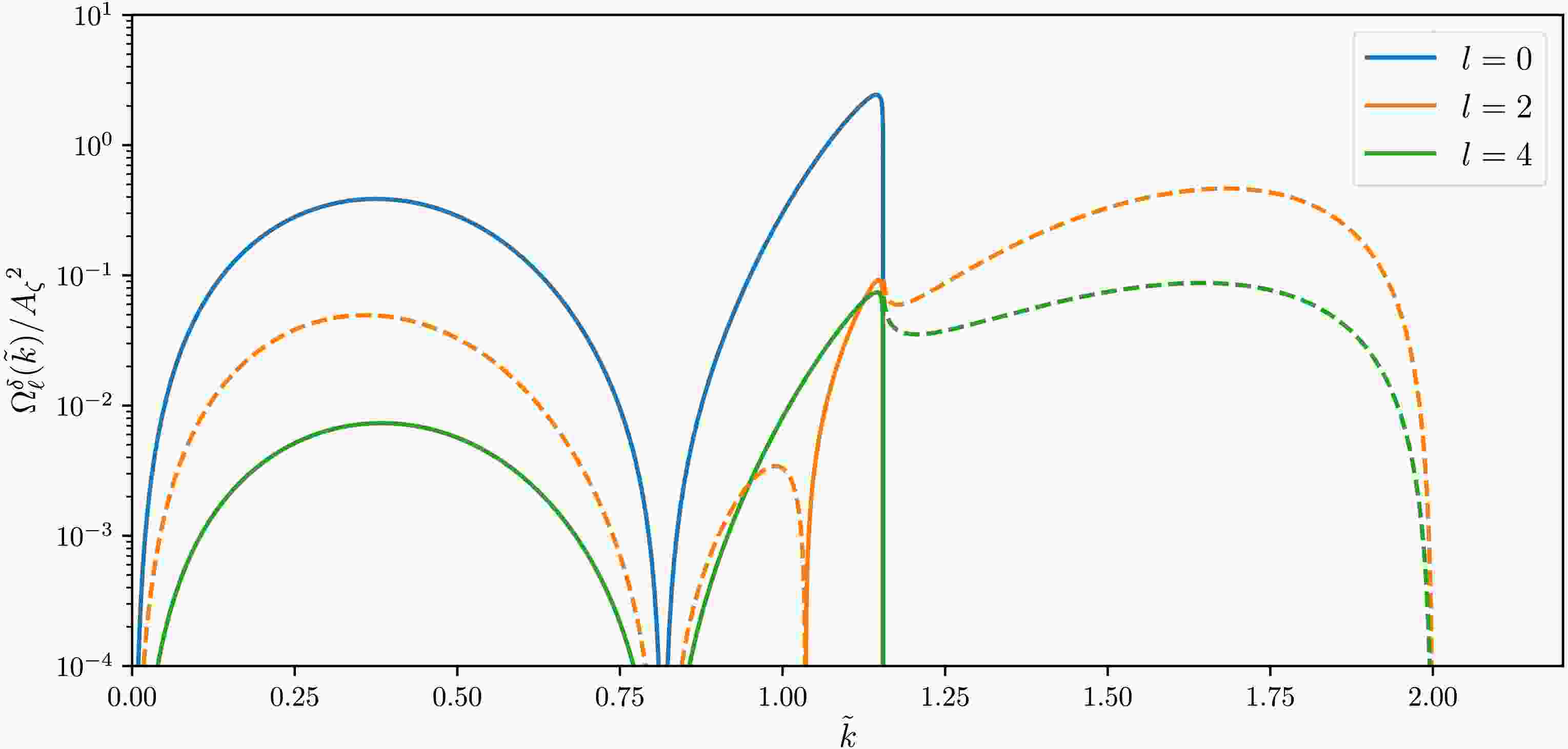
$ \begin{aligned} \Omega_l^\delta(\tilde{k}) &= \Omega_{{\rm{iso}}}^\delta(\tilde{k}) \left( \delta_{l 0} + H_l^\delta(\tilde{k} ) \right) \ , \end{aligned} $
(30) where
$ \begin{aligned}[b] \Omega_{{\rm{iso}}}^\delta(\tilde{k}) =\;& \frac{3A_\zeta^2}{64} \left( \frac{\tilde{k}^2 - 4}{4} \right)^2 \tilde{k}^2 (3\tilde{k}^2 - 2)^2 \\&\times\Bigg( \pi^2 (3\tilde{k}^2 - 2)^2 \, \Theta\left( \frac{2}{\sqrt{3}} - \tilde{k} \right) \\ &+ \left( 4 + (3\tilde{k}^2 - 2) \ln \left| 1 - \frac{4}{3\tilde{k}^2} \right|^2 \right) \Theta(2 - \tilde{k}) \Bigg) \ , \end{aligned} $
(31) $ \begin{eqnarray} H_0^\delta(\tilde{k} )&=&\frac{5A_2^2}{8} \left( 8 - 12\tilde{k}^2 + 3\tilde{k}^4 \right) \ , \end{eqnarray} $
(32) $ \begin{eqnarray} H_2^\delta(\tilde{k} )&=&\frac{A_2}{4} (3\tilde{k}^2 - 4) + \frac{5A_2^2}{56} (8 + 6\tilde{k}^2 - 3\tilde{k}^4) \ , \end{eqnarray} $
(33) $ \begin{eqnarray} H_4^\delta(\tilde{k} )&=&\frac{5A_2^2}{448} (48 + 8\tilde{k}^2 + 3\tilde{k}^4) \ . \end{eqnarray} $
(34) In Fig. 1, we present the results for the multipole moments of the energy density spectrum of second-order scalar-induced gravitational waves, obtained under the assumption of a monochromatic primordial power spectrum in Eq. (23) and Eq. (29).
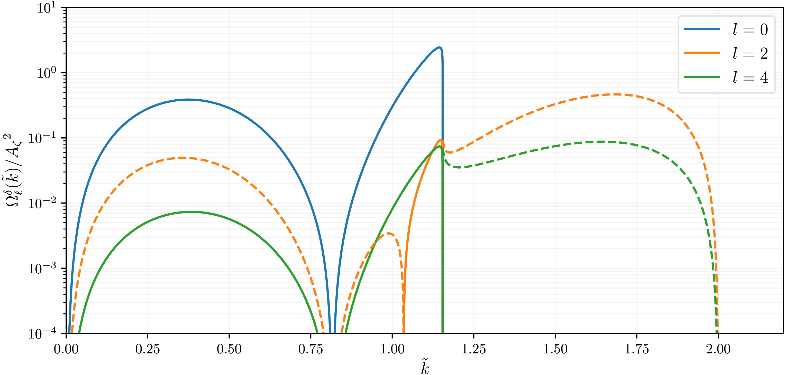
Figure 1. (color online)
$ \Omega_l^\delta $ as a function of$ \tilde{k} $ , assuming$ A_2=0.2 $ . The dashed curves denote the absolute value of the negative ratios of$ l = 0, 2 $ . -
In the previous subsection, we derived the explicit expression for the energy density spectrum of second-order SIGWs, which originates from the small-scale anisotropic primordial power spectrum, after performing spatial averaging. As we mentioned earlier, due to the limited precision of current observational data, such small-scale anisotropies cannot be directly detected. Nevertheless, analyzing the anisotropy of the energy density spectrum of SIGWs at small scales remains meaningful, as it may provide a window for probing small-scale anisotropic inflationary models in the future. In this subsection, we compute the anisotropy of second-order SIGWs at small scales. For simplicity, we focus on the primordial power spectrum with
$ l=0 $ and$ l=2 $ . Such an anisotropic primordial spectrum is typically associated with anisotropic inflationary models involving vector or gauge fields, which are discussed in Sec. IV. Based on Eq. (16), the anisotropic primordial power spectrum in this scenario can be expressed as$ {\cal{P}}^{\hat{{\bf{n}}}}_\zeta({\bf{k}}) = {\cal{P}}_{0,\zeta}(k) \left(1-5A_2(k) \right) {\cal{P}}_l(\hat{{\bf{n}}}\cdot\hat{{\bf{k}}})\ . $
(23) By substituting Eq. (23) into Eq. (11) and simplifying, we obtain
$ \begin{aligned} \Omega^{{\bf{n}}}_{{\rm{GW}}}(\eta, {\bf{k}}) &= \sum\limits_{l=0}^{\infty} (-i)^{l} (2l + 1) \Omega_{l}(\eta, k) P_{l}(\hat{{\bf{n}}} \cdot \hat{{\bf{k}}}) \ . \end{aligned} $
(24) In Eq. (24),
$ \Omega_{l}(\eta, k) $ represents the multipole moment associated with second-order SIGWs, and its explicit form can be expressed as$ \begin{aligned} \Omega_{l}(x, k) &=\frac{x^2}{6} \int_0^\infty {\rm{d}} v \int_{|1 - v|}^{1 + v} {\rm{d}} u \left( \frac{4v^2 - (1 + v^2 - u^2)^2}{4uv} \right)^2 I^2(u,v,x) {\cal{P}}_\zeta(uk) {\cal{P}}_\zeta(vk) \left[ \delta_{l 0} + H_l(u,v,x) \right] \ , \end{aligned} $
(25) where
$ \delta_{l 0} $ is the Kronecker delta.$ H_l $ in Eq. (25) are given by$ \begin{eqnarray} H_{0}&=& A_2(uk)A_2(vk)\frac{160}{81u^2v^2} \left( 3u^4 + 2u^2(v^2 - 3) + 3(v^2 - 1)^2 \right) \ , \end{eqnarray} $
(26) $ \begin{aligned}[b] H_{2}=\;&\frac{32A_2(uk)}{81u^2v^2} \left( 3u^4 v^2 + 2u^2 v^2 (1 - 3v^2) + 3v^2(v^2 - 1)^2 \right)+\frac{32A_2(vk)}{81u^2v^2} \left( 3u^2(1 + v^2 - u^2)^2 - 4u^2 v^2 \right) \\ &-\frac{160A_2(uk)A_2(vk)}{567} \frac{1}{u^2 v^2} \left( 3u^6 - 3u^4(v^2 + 1) + 3(v^2 - 1)^2(v^2 + 1) - u^2(3 + 2v^2 + 3v^4) \right) \ , \end{aligned} $
(27) $ \begin{aligned}[b] H_{4}=\;&\frac{20A_2(uk)A_2(vk)}{567u^2v^2} \Big( 35u^8 - 20u^6(3 + 7v^2) + 6u^4(3 + 10v^2 + 35v^4)+4u^2(1 + 3v^2 + 15v^4 - 35v^6) \\ &+ (v^2 - 1)^2(3 + 10v^2 + 35v^4) \Big) \ . \end{aligned} $
(28) To better illustrate the small-scale anisotropy of second-order SIGWs, we consider the following form of the monochromatic primordial power spectrum:
$ \begin{eqnarray} {\cal{P}}_{0,\zeta}(k)=A_{\zeta}k_*\delta(k-k_*) \ . \end{eqnarray} $
(29) In this case, the multipole moment of the energy density spectrum of second-order SIGWs in Eq. (25) is given by
$ \begin{aligned} \Omega_l^\delta(\tilde{k}) &= \Omega_{{\rm{iso}}}^\delta(\tilde{k}) \left( \delta_{l 0} + H_l^\delta(\tilde{k} ) \right) \ , \end{aligned} $
(30) where
$ \begin{aligned}[b] \Omega_{{\rm{iso}}}^\delta(\tilde{k}) =\;& \frac{3A_\zeta^2}{64} \left( \frac{\tilde{k}^2 - 4}{4} \right)^2 \tilde{k}^2 (3\tilde{k}^2 - 2)^2 \\&\times\Bigg( \pi^2 (3\tilde{k}^2 - 2)^2 \, \Theta\left( \frac{2}{\sqrt{3}} - \tilde{k} \right) \\ &+ \left( 4 + (3\tilde{k}^2 - 2) \ln \left| 1 - \frac{4}{3\tilde{k}^2} \right|^2 \right) \Theta(2 - \tilde{k}) \Bigg) \ , \end{aligned} $
(31) $ \begin{eqnarray} H_0^\delta(\tilde{k} )&=&\frac{5A_2^2}{8} \left( 8 - 12\tilde{k}^2 + 3\tilde{k}^4 \right) \ , \end{eqnarray} $
(32) $ \begin{eqnarray} H_2^\delta(\tilde{k} )&=&\frac{A_2}{4} (3\tilde{k}^2 - 4) + \frac{5A_2^2}{56} (8 + 6\tilde{k}^2 - 3\tilde{k}^4) \ , \end{eqnarray} $
(33) $ \begin{eqnarray} H_4^\delta(\tilde{k} )&=&\frac{5A_2^2}{448} (48 + 8\tilde{k}^2 + 3\tilde{k}^4) \ . \end{eqnarray} $
(34) Fig. 1 presents the results for the multipole moments of the energy density spectrum of second-order SIGWs, obtained assuming a monochromatic primordial power spectrum in Eq. (23) and Eq. (29).
Figure 1. (color online)
$ \Omega_l^\delta $ as a function of$ \tilde{k} $ , assuming$ A_2=0.2 $ . The dashed curves denote the absolute value of the negative ratios of$ l = 0, 2 $ . -
To calculate the power spectrum of the second-order SIGWs, we need to provide the specific expression of the primordial power spectrum. In this paper, we consider the log-normal primordial power spectrum [50−53]
$ \begin{aligned} {\cal{P}}_{0,\zeta}(k) = \frac{A_\zeta}{\sqrt{2\pi\sigma^2}}\exp{\left(-\frac{\ln^2(k/k_*)}{2\sigma^2}\right)}\ , \end{aligned} $
(35) where
$ A_\zeta $ is the amplitude of the primordial power spectrum,$ k_* = 2\pi f_* $ is the wavenumber at which the power spectrum has a log-normal peak, and σ characterizes the width of the log-normal distribution. The anisotropy of the primordial power spectrum on small scales is characterized by the parameters$ C_l $ $ (l=1,2,3,4) $ in Eq. (17). The energy density of second-order SIGW during the RD era can be calculated in terms of Eq. (22). Taking into account the thermal history of the universe, we obtain the current total energy density spectrum of SIGWs [54]$ \Omega_{0,{\rm{GW}}}(k) = \Omega_{rad,0}\left(\frac{g_{*,\rho,e}}{g_{*,\rho,0}}\right)\left(\frac{g_{*,s,0}}{g_{*,s,e}}\right)^{4/3}\Omega_{{\rm{GW}}}(k, \eta)\ , $
(36) where
$ \Omega_{rad,0} = 4.2 \times 10^{-5} h^{-2} $ is the energy density fraction of radiation today, and the dimensionless Hubble constant is$ h = 0.6736 $ [20]. The$ g_{*,\rho} $ and$ g_{*,s} $ are the effective numbers of relativistic degrees of freedom [55]. In Fig. 2, we illustrate the impact of different$ C_l $ $ (l=1,2,3,4) $ parameters on the energy density spectrum of second-order SIGWs under a log-normal primordial power spectrum. In this paper, we consider the following two types of anisotropic inflation models: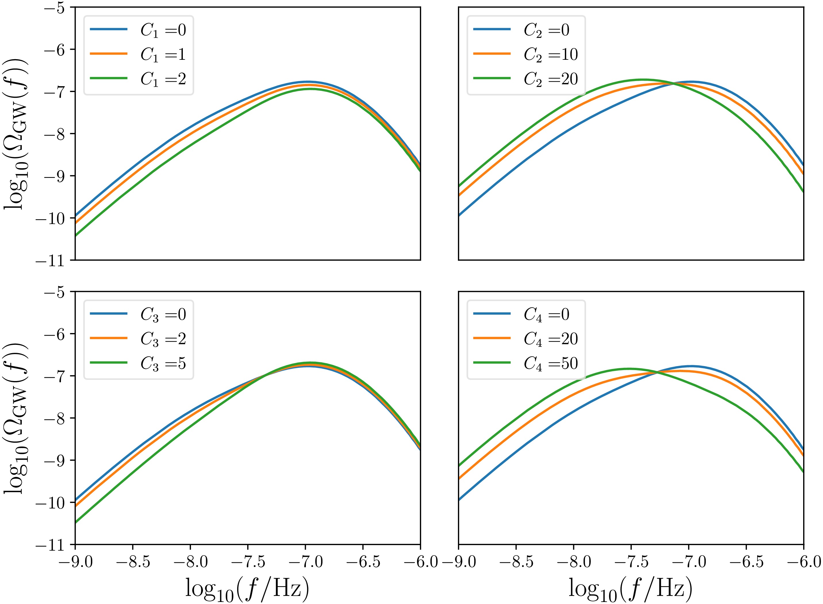
Figure 2. (color online) The impact of different
$ C_l $ parameters on the energy density spectrum is shown. Here,$ f_* $ ,$ A_\zeta $ , and σ are fixed at$ 10^{-7} $ Hz,$ 0.5 $ , and 1, respectively. In each subplot, only$ C_1 $ ,$ C_2 $ ,$ C_3 $ , or$ C_4 $ is non-zero, from left to right. Different colors in the figure represent different values of the$ C_l $ parameter, as indicated in the legend.1, Gauge field: Introducing a vector (gauge) field during inflation can serve as a mechanism for generating cosmic anisotropy. In this type of model, the primordial power spectrum can be parameterized as follows [56]
$ \begin{aligned} {\cal{P}}^{\hat{{\bf{n}}}}_\zeta({\bf{k}}) = {\cal{P}}_{0,\zeta}(k)\left(1 +C_2{\cal{P}}_2(\hat{{\bf{n}}}\cdot\hat{{\bf{k}}})\right) \ . \end{aligned} $
(37) 2, Finslerian inflation: Modifying the spacetime background during inflation can introduce anisotropy. One of the most prominent spacetime backgrounds for this purpose is the Finsler spacetime background. In this model, the form of the anisotropic primordial power spectrum is given by [57]
$ \begin{aligned} {\cal{P}}^{\hat{{\bf{n}}}}_\zeta({\bf{k}}) = {\cal{P}}_{0,\zeta}(k)\left(1 +C_1{\cal{P}}_1(\hat{{\bf{n}}}\cdot\hat{{\bf{k}}})\right) \ . \end{aligned} $
(38) The aforementioned two inflation models have presented the anisotropic primordial power spectra under the conditions of
$ C_2\ne 0 $ and$ C_1\ne 0 $ , respectively. In the rest of this section, we will discuss the impact of these two models on PTA and LISA observations separately, and consider model-independent scenarios where both$ C_1 $ and$ C_2 $ are non-zero. -
To calculate the power spectrum of the second-order SIGWs, the specific expression of the primordial power spectrum is required. In this study, we consider the log-normal primordial power spectrum [48−51]:
$ \begin{aligned} {\cal{P}}_{0,\zeta}(k) = \frac{A_\zeta}{\sqrt{2\pi\sigma^2}}\exp{\left(-\frac{\ln^2(k/k_*)}{2\sigma^2}\right)}\ , \end{aligned} $
(35) where
$ A_\zeta $ is the amplitude of the primordial power spectrum,$ k_* = 2\pi f_* $ is the wavenumber at which the power spectrum exhibits a log-normal peak, and σ characterizes the width of the log-normal distribution. The anisotropy of the primordial power spectrum on small scales is characterized by$ C_l $ $ (l=1,2,3,4) $ in Eq. (17). The energy density of second-order SIGWs during the RD era can be calculated using Eq. (22). Considering the thermal history of the Universe, we obtain the current total energy density spectrum of SIGWs as [52]$ \Omega_{0,{\rm{GW}}}(k) = \Omega_{rad,0}\left(\frac{g_{*,\rho,e}}{g_{*,\rho,0}}\right)\left(\frac{g_{*,s,0}}{g_{*,s,e}}\right)^{4/3}\Omega_{{\rm{GW}}}(k, \eta)\ , $
(36) where
$ \Omega_{rad,0} = 4.2 \times 10^{-5} h^{-2} $ is the energy density fraction of radiation today, and the dimensionless Hubble constant is$ h = 0.6736 $ [20];$ g_{*,\rho} $ and$ g_{*,s} $ are the effective numbers of relativistic degrees of freedom [53]. Fig. 2 illustrates the impact of different$ C_l $ $ (l=1,2,3,4) $ on the energy density spectrum of second-order SIGWs under a log-normal primordial power spectrum. In this study, we consider the following two types of anisotropic inflation models:
Figure 2. (color online) Impact of different
$ C_l $ parameters on the energy density spectrum. Here,$ f_* $ ,$ A_\zeta $ , and σ are fixed at$ 10^{-7} $ Hz,$ 0.5 $ , and 1, respectively. In each subplot, only$ C_1 $ ,$ C_2 $ ,$ C_3 $ , or$ C_4 $ is non-zero, from left to right. Different colors in the figure represent different values of the$ C_l $ parameter, as indicated in the legend.1, Gauge field: Introducing a vector (gauge) field during inflation can serve as a mechanism for generating cosmic anisotropy. In this type of model, the primordial power spectrum can be parameterized as follows [32]:
$ \begin{aligned} {\cal{P}}^{\hat{{\bf{n}}}}_\zeta({\bf{k}}) = {\cal{P}}_{0,\zeta}(k)\left(1 +C_2{\cal{P}}_2(\hat{{\bf{n}}}\cdot\hat{{\bf{k}}})\right) . \end{aligned} $
(37) 2, Finslerian inflation: Modifying the spacetime background during inflation can introduce anisotropy. One of the most prominent spacetime backgrounds for this purpose is the Finsler spacetime background. In this model, the form of the anisotropic primordial power spectrum is given by [54]
$ \begin{aligned} {\cal{P}}^{\hat{{\bf{n}}}}_\zeta({\bf{k}}) = {\cal{P}}_{0,\zeta}(k)\left(1 +C_1{\cal{P}}_1(\hat{{\bf{n}}}\cdot\hat{{\bf{k}}})\right) . \end{aligned} $
(38) The aforementioned two inflation models provide anisotropic primordial power spectra under the conditions
$ C_2\ne 0 $ and$ C_1\ne 0 $ , respectively. In the remainder of this section, we discuss the impact of these two models on PTA and Laser Interferometer Space Antenna (LISA) observations separately and consider model-independent scenarios, where both$ C_1 $ and$ C_2 $ are non-zero. -
To constrain the parameter space of the anisotropic primordial power spectrum using PTA observations, we employ the kernel density estimator (KDE) representations of the free spectra and construct the likelihood function [55−57]:
$ \ln {\cal{L}}(d|\theta) = \sum\limits_{i=1}^{N_f} p(\Phi_i,\theta)\ . $
(39) In Eq. (39),
$ p(\Phi_i,\theta) $ represents the probability density of$ \Phi_i $ for a given θ, and$ \Phi_i = \Phi(f_i) $ denotes the time delay:$ \Phi(f) = \sqrt{\frac{H_0^2 \Omega_{{\rm{GW}}}(f)}{8\pi^2 f^5 T_{{\rm{obs}}}}} \ , $
(40) where
$ H_0=h\times 100 $ km/s/Mpc is the present-day value of the Hubble constant. Specifically, we directly utilize the publicly available KDE representations of the free spectrum provided by the NANOGrav 15-year dataset [58]. These KDEs are constructed based on an analysis explicitly accounting for Hellings–Downs (HD) spatial correlations. By adopting these official HD-correlated KDEs, our analysis strictly preserves the spatial information inherent in the PTA data, ensuring that the constraints are derived from a signal consistent with a GW background rather than from uncorrelated common red noise. Bayesian analysis is performed using ʙɪʟʙʏ [59] with its integrated ᴅʏɴᴇsᴛʏ nested sampler [60–61]. For the anisotropic primordial power spectra, the posterior distributions are presented in Figs. 3–5, with prior distributions for$ \log_{10}(f_*/{\rm{Hz}}) $ ,$ \log_{10}(A_{\zeta}) $ , σ,$ \log_{10}(C_1) $ , and$ \log_{10}(C_2) $ set as uniform over the intervals$ [-10, -5] $ ,$ [-4, 0] $ ,$ [0.1, 10] $ ,$ [-3, 1] $ , and$ [-2, 3] $ , respectively; here, we set$ C_l=0 $ $ (l>2) $ . The corresponding energy density spectra of second-order SIGWs are shown in Fig. 6. As illustrated in Figs. 3–5, PTA observations can effectively constrain the parameters$ A_{\zeta} $ , σ, and$ f_* $ that characterize the isotropic primordial power spectrum. However, owing to the presence of parameter degeneracies, the current PTA data cannot effectively constrain the parameters$ C_1 $ and$ C_2 $ , which describe small-scale anisotropies. This result is mainly attributed to two factors. First, the current PTA observational data are not sufficiently precise. Second, the introduction of the anisotropy parameter$ C_l $ leads to increased degeneracy in the energy density spectrum of SIGWs. To better constrain the primordial power spectrum anisotropy on small scales, additional cosmological observations that can place limits on the energy density spectrum of SIGWs must be considered.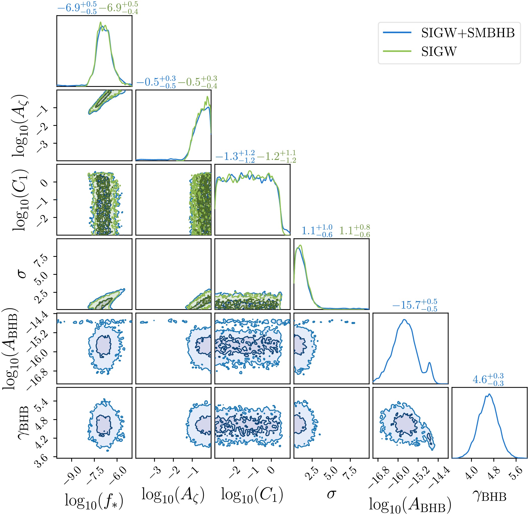
Figure 3. (color online) Corner plot showing the posterior distributions with
$ C_1 \neq 0 $ . The blue and green curves correspond to the NANOGrav 15-year dataset. Off-diagonal panels display 1-σ and 2-σ confidence intervals for joint distributions, and diagonal panels provide marginal distributions with the median values and 1-σ uncertainties noted above each histogram.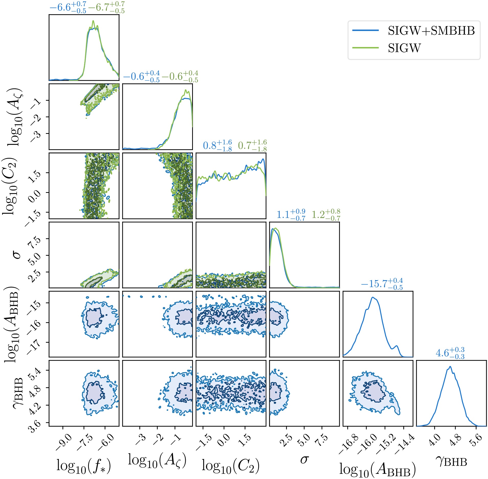
Figure 4. (color online) Corner plot showing the posterior distributions with
$ C_2 \neq 0 $ . The blue and green curves correspond to the NANOGrav 15-year dataset. Off-diagonal panels display 1-σ and 2-σ confidence intervals for joint distributions, and diagonal panels provide marginal distributions with the median values and 1-σ uncertainties noted above each histogram.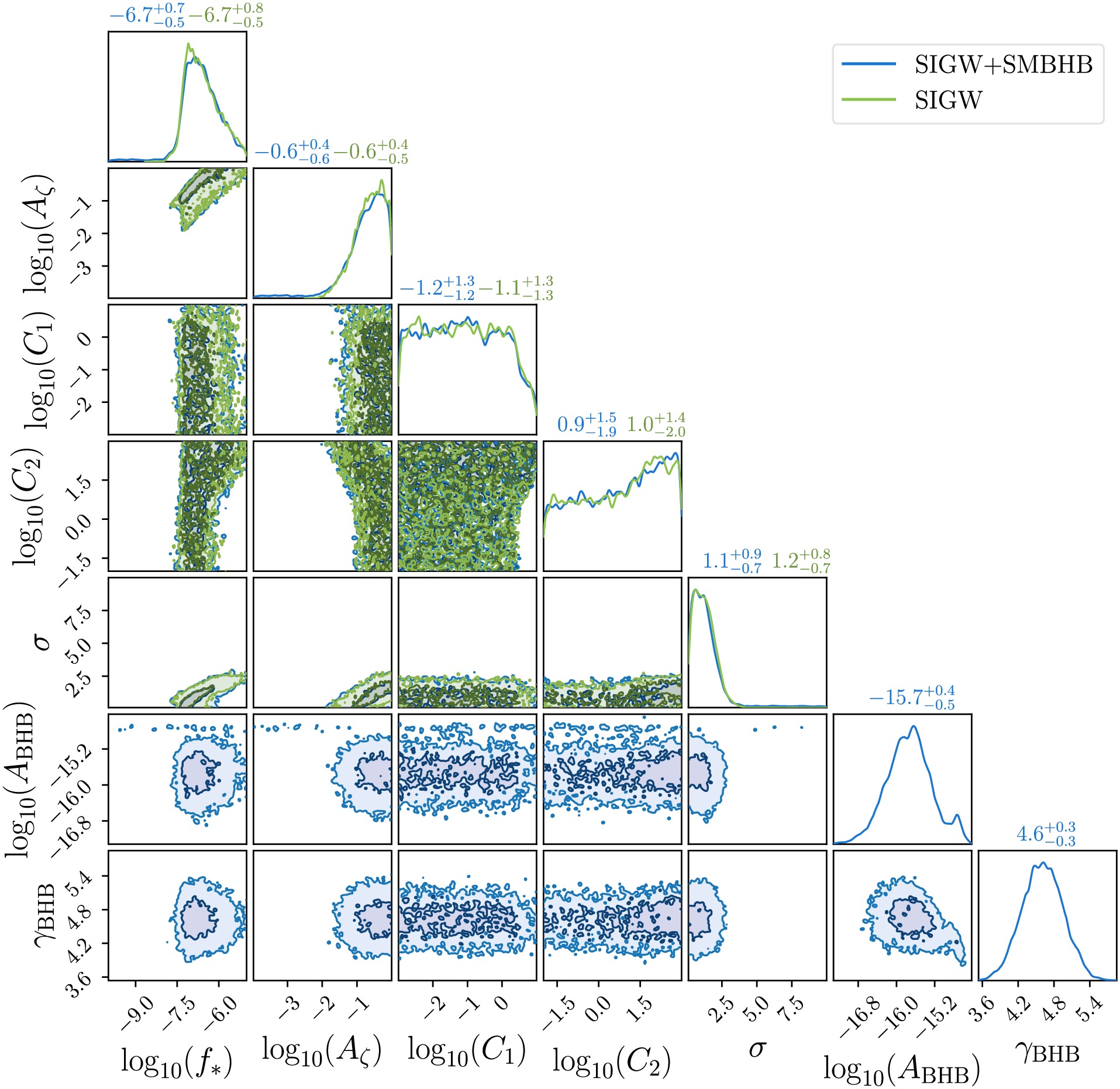
Figure 5. (color online) Corner plot showing the posterior distributions with
$ C_{l} \neq 0 $ $ (l=1,2) $ . The blue and green curves correspond to the NANOGrav 15-year dataset. Off-diagonal panels display 1-σ and 2-σ confidence intervals for joint distributions. Diagonal panels provide marginal distributions with the median values and 1-σ uncertainties noted above each histogram.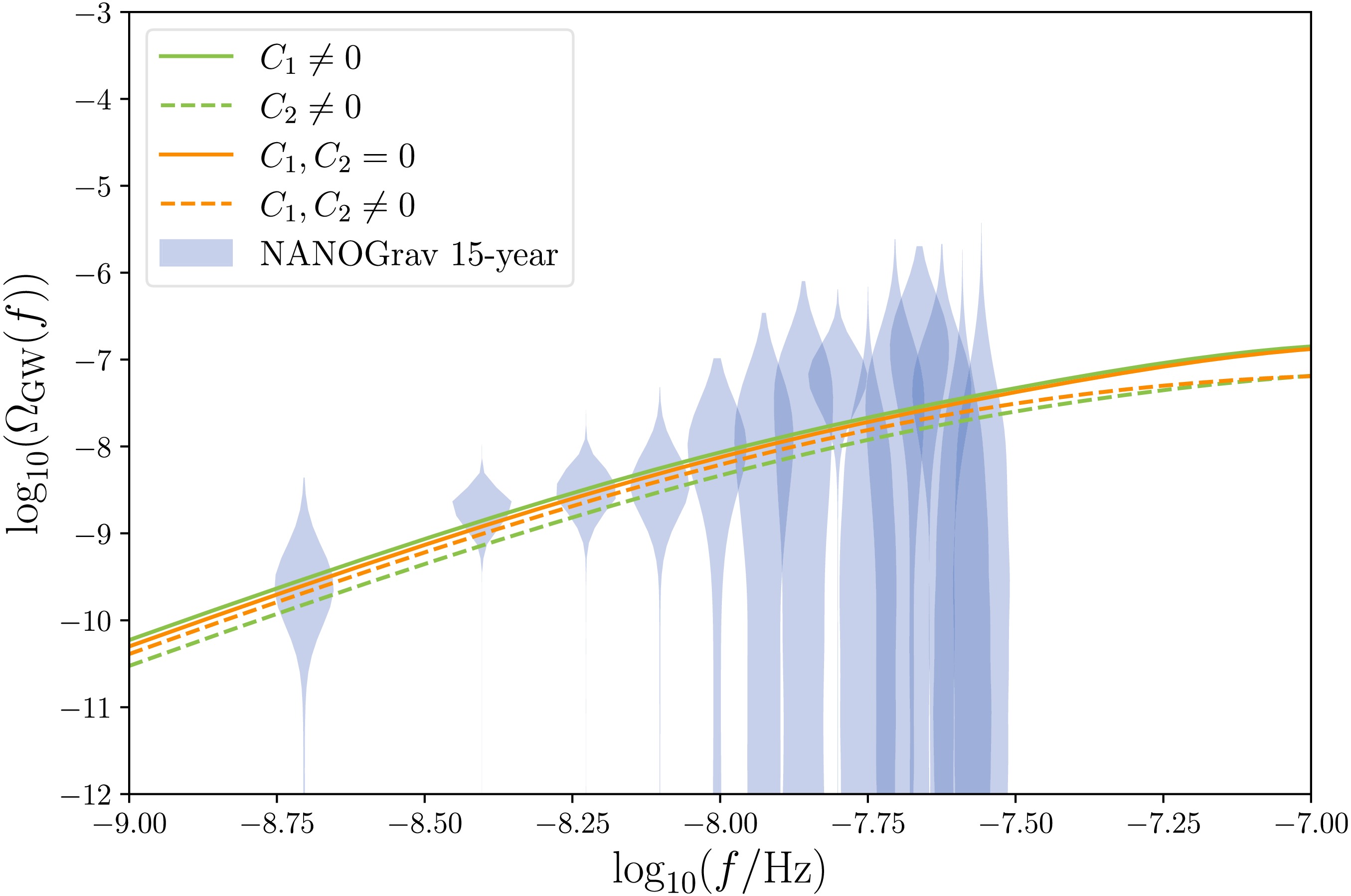
Figure 6. (color online) The energy density spectra of second-order SIGWs with anisotropic primordial power spectra. The curves are based on parameters derived from the median values of the posterior distributions of the NANOGrav 15-year dataset. The energy density spectra derived from the free spectrum of the NANOGrav 15-year dataset is shown with blue shading. Different line styles and colors indicate scenarios with
$ C_1, C_2 = 0 $ ,$ C_1 \neq 0 $ ,$ C_2 \neq 0 $ , and$ C_1, C_2 \neq 0 $ , as labeled in the figure.In this section, we consider the constraints from large-scale cosmological observations on second-order SIGWs and the corresponding parameter space of the small-scale anisotropic primordial power spectrum. Large-scale cosmological observations constrain the SGWB via two types of methods. The first method treats the SGWB as an additional radiation component, modifying the effective number of relativistic species,
$ N_{{\rm{eff}}} $ . To remain consistent with current observational bounds, the total energy density spectrum must satisfy [62–63]$ \int_{f_{{\rm{min}}}}^{\infty} h^2\Omega_{{\rm{GW}},0}(k) {\rm{d}} \left(\ln k\right) \lt 1.3 \times 10^{-6}\frac{\Delta N_{{\rm{eff}}}}{0.234} \ , $
(41) where
$ \Delta N_{{\rm{eff}}}= N_{{\rm{eff}}}-3.046 $ . Here, we use the$ N_{{\rm{eff}}} $ limits provided by Aghanim et al. [20], who report$ N_{{\rm{eff}}}=3.04 \pm 0.22 $ at a 95% confidence level for the$\mathtt{Planck}$ + BAO + Big-Bang nucleosynthesis data. The second method directly utilizes CMB and BAO measurements, imposing the following stricter constraint:$ \int_{f_{{\rm{min}}}}^{\infty} h^2\Omega_{{\rm{GW}},0}(k) {\rm{d}}\left(\ln k\right) \lt 2.9\times 10^{-7} \ , $
(42) at 95% confidence level for CMB+BAO data [64]. Figs. 7–9 present the current constraints from large-scale cosmological observations on the parameter space composed of
$ C_1 $ and$ C_2 $ . The green and red lines correspond to the observational limits given by Eq. (41) and Eq. (42), respectively.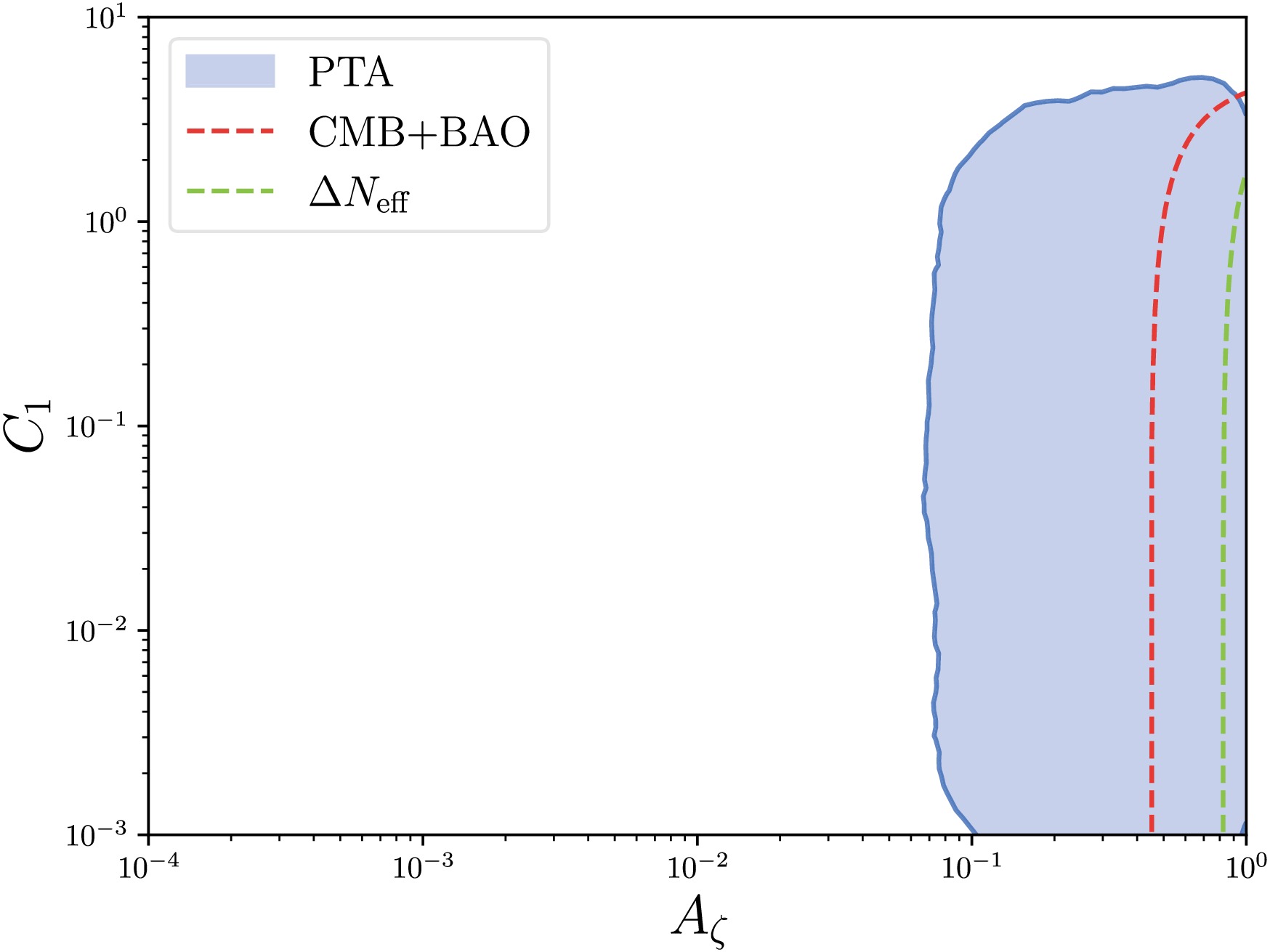
Figure 7. (color online) Constraints on
$ A_\zeta $ and$ C_1 $ assuming$ \sigma=1 $ and$ C_2=0 $ . The blue shaded region represents the 95% credible intervals corresponding to the two-dimensional posterior distribution shown in Fig. 3 with the KDE method. The red and green lines denote the lower bounds of$ C_1 $ from CMB and BAO observations (Eq. (42)) and those from$ \Delta N_{\mathrm{eff}} $ (Eq. (41)), respectively.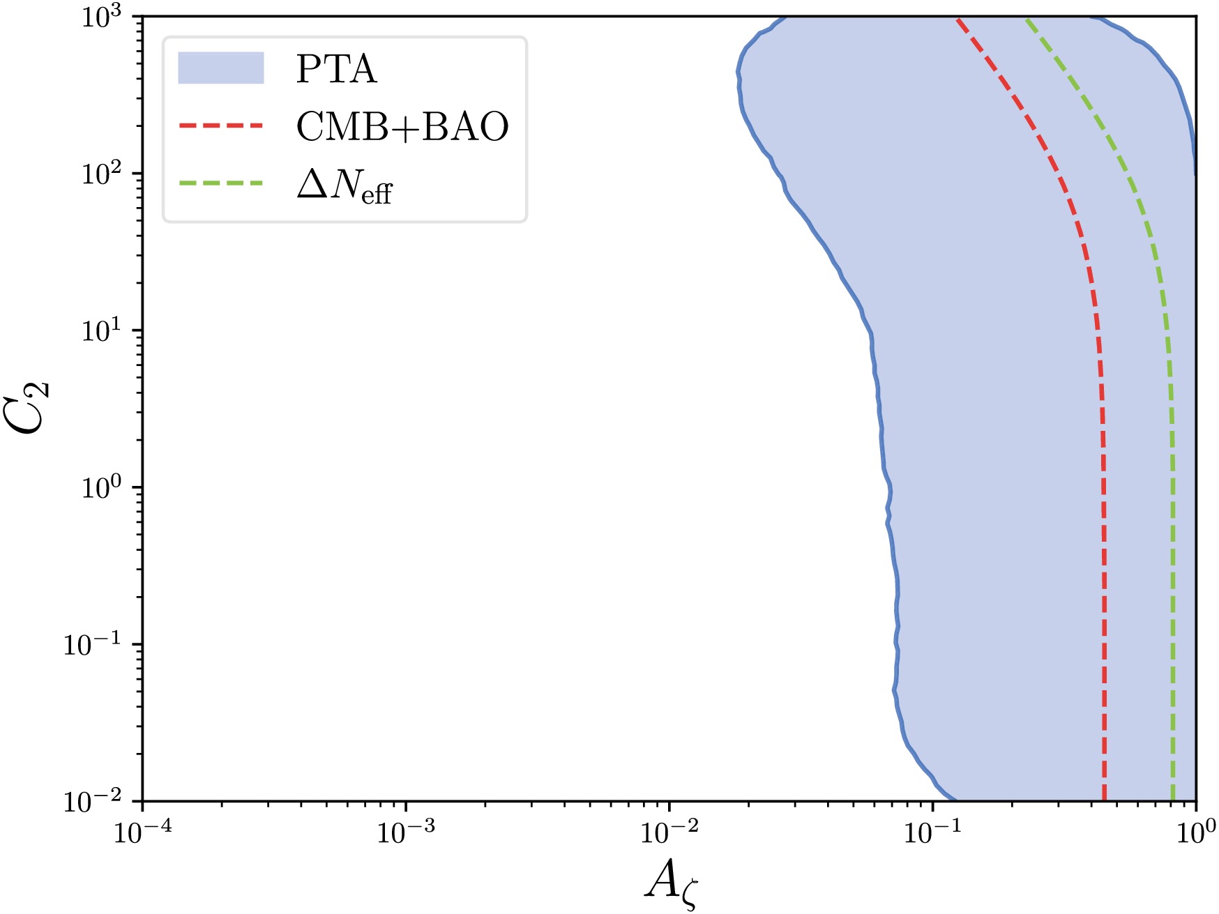
Figure 8. (color online) Constraints on
$ A_\zeta $ and$ C_2 $ assuming$ \sigma=1 $ and$ C_1=0 $ . The blue shaded region represents the 95% credible intervals corresponding to the two-dimensional posterior distribution shown in Fig. 4 with the KDE method. The red and green lines denote the upper bounds of$ C_2 $ from CMB and BAO observations (Eq. (42)) and from$ \Delta N_{\mathrm{eff}} $ (Eq. (41)), respectively.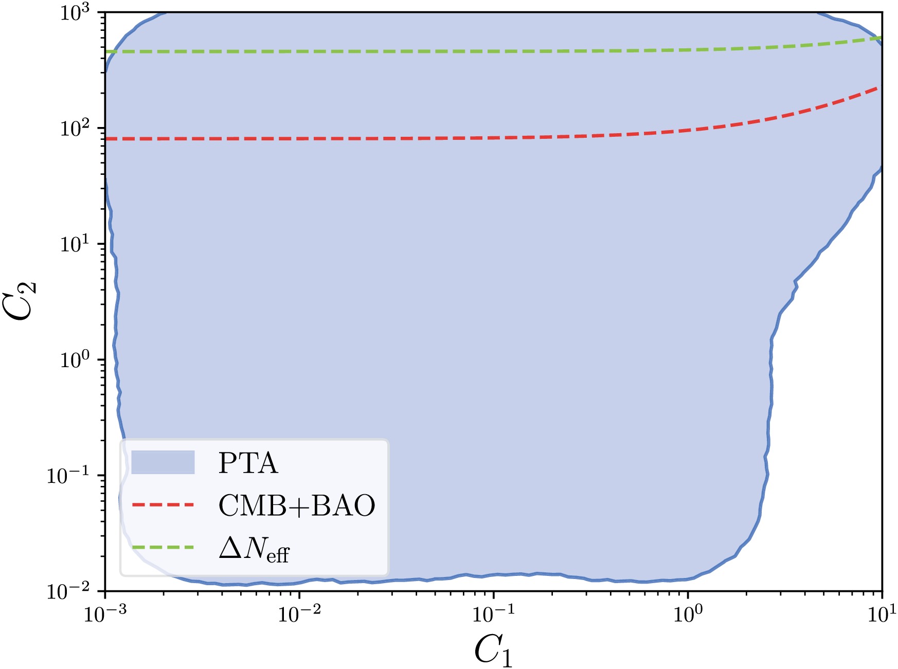
Figure 9. (color online) Constraints on
$ C_1 $ and$ C_2 $ assuming$ \sigma=1 $ and$ A_\zeta=10^{-0.5} $ . The blue shaded regions represent the 95% credible intervals corresponding to the two-dimensional posterior distribution shown in Fig. 5 with the KDE method. The black solid line and gray dashed line denote the upper bounds of$ C_2 $ from CMB and BAO observations (Eq. (42)) and from$ \Delta N_{{\rm{eff}}} $ (Eq. (41)), respectively.Furthermore, to better assess the plausibility of different models in explaining current PTA observations, we perform a detailed analysis of the Bayes factors between different models. The Bayes factor is defined as
$ B_{i,j} = \frac{Z_i}{Z_j} $ , where$ Z_i $ represents the evidence of model$ H_i $ . In addition to SIGWs, we investigate a hybrid model scenario, wherein both SMBHBs and SIGWs contribute jointly. The energy density spectrum of SMBHBs is characterized by [7]$ \Omega_{{\rm{GW}}}^{{\rm{BH}}}(f) = \frac{2\pi^2 A_{{\rm{BHB}}}^2}{3H_0^2 h^2} (\frac{f}{{\rm{year}}^{-1}})^{5-\gamma_{{\rm{BHB}}}}{\rm{year}}^{-2} \ , $
(43) with the prior distribution for
$ \log_{10}A_{{\rm{BHB}}} $ assumed to follow a multivariate Gaussian distribution [7]:$ \begin{aligned} {\boldsymbol{\mu}}_{{\rm{BHB}}}&=\begin{pmatrix} -15.6 \\ 4.7 \end{pmatrix} \ , \\ {\boldsymbol{\sigma}}_{{\rm{BHB}}}&=0.1\times \begin{pmatrix} 2.8 & -0.026\\ -0.026 & 2.8 \end{pmatrix} \ . \end{aligned} $
(44) As shown in Fig. 10, we calculate the Bayes factors between different models. The results indicate that when small-scale anisotropies in the primordial power spectrum are considered, the Bayesian factor for SIGWs within the considered parameter space is approximately
$ 10 $ . This result suggests that compared to the SMBHB model, SIGWs with different anisotropic parameters are more likely to dominate current PTA observations. To directly assess the statistical preference for small-scale anisotropy, the Bayes factor between the anisotropic models and isotropic SIGW model ($ C_1=C_2=0 $ ) can be derived simply by taking the ratio of the Bayes factors presented in Fig. 10. The Bayes factor for the most favored anisotropic case ($ C_2 \neq 0 $ ) relative to the isotropic case is approximately$ {\cal{B}} \approx 14.31/13.24 \approx 1.08 $ , which is close to unity. This value indicates that current PTA data are insufficient to effectively distinguish between isotropic and anisotropic primordial power spectra on small scales.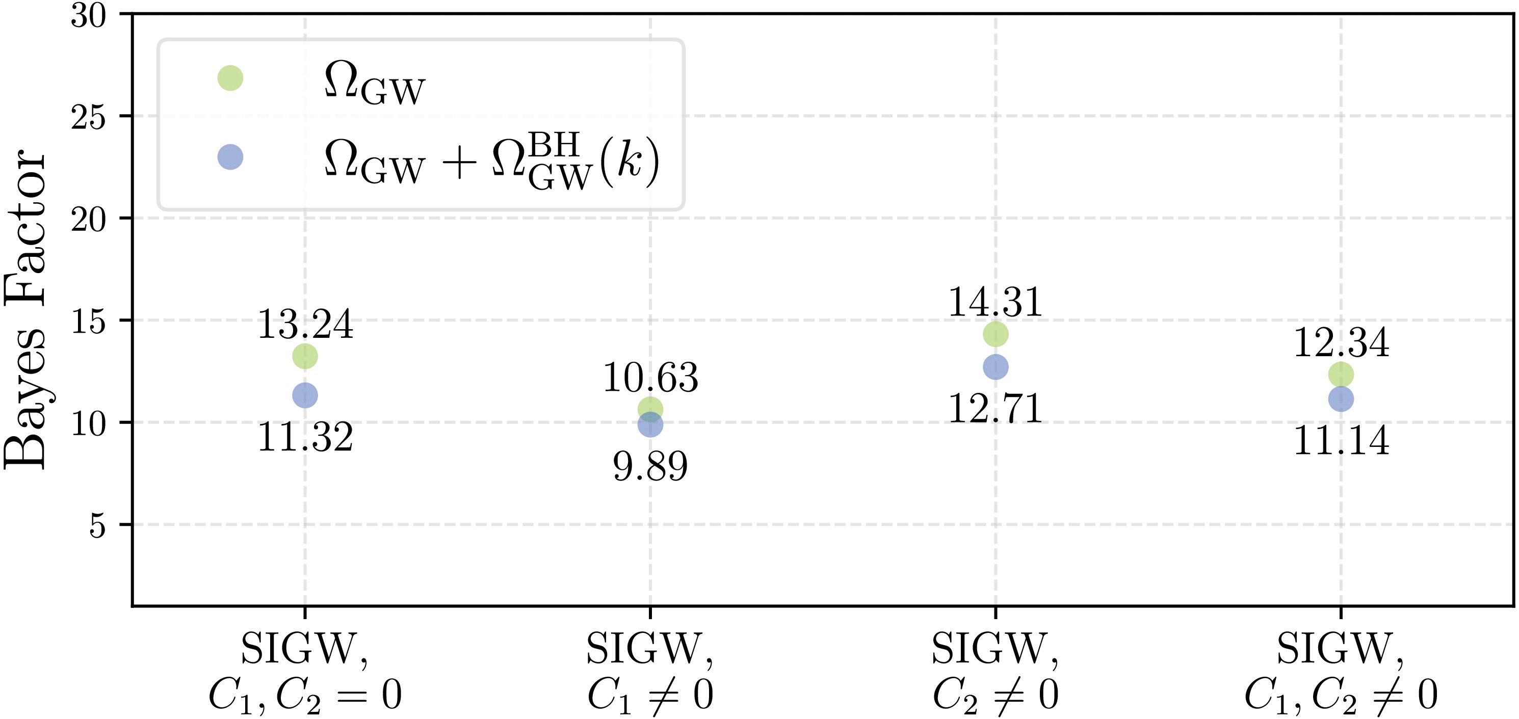
Figure 10. (color online) Bayes factors between different models. The vertical axis represents the Bayes factor of different models relative to SMBHB, and the horizontal axis represents the different models. The green dots correspond to models without SMBHB, and the blue dots represent models in combination with the SMBHB signal.
-
To constrain the parameter space of the anisotropic primordial power spectrum using PTA observations, we employ the kernel density estimator (KDE) representations of the free spectra to construct the likelihood function [58−60]
$ \ln {\cal{L}}(d|\theta) = \sum\limits_{i=1}^{N_f} p(\Phi_i,\theta)\ . $
(39) In Eq. (39),
$ p(\Phi_i,\theta) $ represents the probability density of$ \Phi_i $ given the parameter θ, and$ \Phi_i = \Phi(f_i) $ denotes the time delay$ \Phi(f) = \sqrt{\frac{H_0^2 \Omega_{{\rm{GW}}}(f)}{8\pi^2 f^5 T_{{\rm{obs}}}}} \ , $
(40) where
$ H_0=h\times 100 $ km/s/Mpc is the present-day value of the Hubble constant. Specifically, we directly utilize the publicly available KDE representations of the free spectrum provided by the NANOGrav 15-year dataset [61]. These KDEs are constructed from the analysis that explicitly accounts for Hellings-Downs spatial correlations. By adopting these official HD-correlated KDEs, our analysis strictly preserves the spatial information inherent in the PTA data, ensuring that the constraints are derived from a signal consistent with a gravitational wave background rather than uncorrelated common red noise. The Bayesian analysis is performed via ʙɪʟʙʏ [62] using its integrated ᴅʏɴᴇsᴛʏ nested sampler [63, 64]. For the anisotropic primordial power spectra, the posterior distributions are presented in Fig. 3–Fig. 5, with prior distributions for$ \log_{10}(f_*/{\rm{Hz}}) $ ,$ \log_{10}(A_{\zeta}) $ , σ,$ \log_{10}(C_1) $ and$ \log_{10}(C_2) $ set as uniform over the intervals$ [-10, -5] $ ,$ [-4, 0] $ ,$ [0.1, 10] $ ,$ [-3, 1] $ , and$ [-2, 3] $ , respectively. Here, we have set$ C_l=0 $ $ (l>2) $ . The corresponding energy density spectra of second-order SIGWs are given in Fig. 6. As illustrated in Fig. 3–Fig. 5, PTA observations are able to effectively constrain the parameters$ A_{\zeta} $ , σ, and$ f_* $ that characterize the isotropic primordial power spectrum. However, due to the presence of parameter degeneracies, the current PTA data fail to provide effective constraints on the parameters$ C_1 $ and$ C_2 $ that describe small-scale anisotropies. There are two main reasons for this result. First, the current PTA observational data are not sufficiently precise. Second, the introduction of the anisotropy parameter$ C_l $ leads to increased degeneracy in the energy density spectrum of SIGWs. To better constrain the primordial power spectrum anisotropies on small scales, it is necessary to consider additional cosmological observations that can place limits on the energy density spectrum of SIGWs.
Figure 3. (color online) Corner plot showing the posterior distributions with
$ C_1 \neq 0 $ . The blue and green curves correspond to the NANOGrav 15-year dataset. Off-diagonal panels display 1-σ and 2-σ confidence intervals for joint distributions, while diagonal panels provide marginal distributions with median values and 1-σ uncertainties noted above each histogram.
Figure 4. (color online) Corner plot showing the posterior distributions with
$ C_2 \neq 0 $ . The blue and green curves correspond to the NANOGrav 15-year dataset. Off-diagonal panels display 1-σ and 2-σ confidence intervals for joint distributions, while diagonal panels provide marginal distributions with median values and 1-σ uncertainties noted above each histogram.
Figure 5. (color online) Corner plot showing the posterior distributions with
$ C_{l} \neq 0 $ $ (l=1,2) $ . The blue and green curves correspond to the NANOGrav 15-year dataset. Off-diagonal panels display 1-σ and 2-σ confidence intervals for joint distributions, while diagonal panels provide marginal distributions with median values and 1-σ uncertainties noted above each histogram.
Figure 6. (color online) The energy density spectra of second-order SIGWs with anisotropic primordial power spectra. The curves are based on parameters derived from the median values of the posterior distributions of the NANOGrav 15-year dataset. The energy density spectra derived from the free spectrum of the NANOGrav 15-year dataset is shown with blue shading. Different line styles and colors indicate scenarios with
$ C_1, C_2 = 0 $ ,$ C_1 \neq 0 $ ,$ C_2 \neq 0 $ , and$ C_1, C_2 \neq 0 $ , as labeled in the figure.In this section, we consider the constraints from large-scale cosmological observations on second-order SIGWs and the corresponding parameter space of the small-scale anisotropic primordial power spectrum. Large-scale cosmological observations constrain the SGWB via two kinds of methods. The first treats the SGWB as an additional radiation component, modifying the effective number of relativistic species,
$ N_{{\rm{eff}}} $ . To remain consistent with current observational bounds, the total energy density spectrum must satisfy [65, 66]$ \int_{f_{{\rm{min}}}}^{\infty} h^2\Omega_{{\rm{GW}},0}(k) {\rm{d}} \left(\ln k\right) \lt 1.3 \times 10^{-6}\frac{\Delta N_{{\rm{eff}}}}{0.234} \ , $
(41) where
$ \Delta N_{{\rm{eff}}}= N_{{\rm{eff}}}-3.046 $ . Here, we use the$ N_{{\rm{eff}}} $ limits provided by [20], which report$ N_{{\rm{eff}}}=3.04 \pm 0.22 $ at a 95% confidence level for the$\mathtt{Planck}$ + BAO + Big-Bang nucleosynthesis (BBN) data. The second method directly utilizes CMB and BAO measurements, imposing the following stricter constraint$ \int_{f_{{\rm{min}}}}^{\infty} h^2\Omega_{{\rm{GW}},0}(k) {\rm{d}}\left(\ln k\right) \lt 2.9\times 10^{-7} \ , $
(42) at 95% confidence level for CMB+BAO data [67]. As shown in Fig. 7–Fig. 9, we present the current constraints from large-scale cosmological observations on the parameter space composed of
$ C_1 $ and$ C_2 $ , where the green line and the red line correspond to the observational limits given by Eq. (41) and Eq. (42), respectively.
Figure 7. (color online) The constraints on
$ A_\zeta $ and$ C_1 $ assuming$ \sigma=1 $ and$ C_2=0 $ . The blue shaded region represents the 95% credible intervals corresponding to the two-dimensional posterior distribution shown in Fig. 3 with the KDE method. The red and green lines denote the lower bounds of$ C_1 $ from CMB and BAO observations in Eq. (42) and$ \Delta N_{\mathrm{eff}} $ in Eq. (41).
Figure 8. (color online) The constraints on
$ A_\zeta $ and$ C_2 $ assuming$ \sigma=1 $ and$ C_1=0 $ . The blue shaded region represents the 95% credible intervals corresponding to the two-dimensional posterior distribution shown in Fig. 4 with the KDE method. The red and green lines denote the upper bounds of$ C_2 $ from CMB and BAO observations in Eq. (42) and$ \Delta N_{\mathrm{eff}} $ in Eq. (41).
Figure 9. (color online) The constraints on
$ C_1 $ and$ C_2 $ assuming$ \sigma=1 $ and$ A_\zeta=10^{-0.5} $ . The blue shaded regions represent the 95% credible intervals corresponding to the two-dimensional posterior distribution shown in Fig. 5 with the KDE method. The black solid line and grey dashed line denote the upper bounds of$ C_2 $ from CMB and BAO observations in Eq. (42) and$ \Delta N_{{\rm{eff}}} $ in Eq. (41).Furthermore, to better assess the plausibility of different models in explaining current PTA observations, we perform a detailed analysis of Bayes factors between different models. The Bayes factor is defined as
$ B_{i,j} = \frac{Z_i}{Z_j} $ , where$ Z_i $ represents the evidence of model$ H_i $ . In addition to scalar-induced gravitational waves, we also investigate a hybrid model scenario where both SMBHBs and SIGWs contribute jointly. The energy density spectrum of SMBHBs is characterized by [7]$ \Omega_{{\rm{GW}}}^{{\rm{BH}}}(f) = \frac{2\pi^2 A_{{\rm{BHB}}}^2}{3H_0^2 h^2} (\frac{f}{{\rm{year}}^{-1}})^{5-\gamma_{{\rm{BHB}}}}{\rm{year}}^{-2} \ , $
(43) with the prior distribution for
$ \log_{10}A_{{\rm{BHB}}} $ assumed to follow a multivariate Gaussian distribution [7]$ \begin{aligned} {\boldsymbol{\mu}}_{{\rm{BHB}}}&=\begin{pmatrix} -15.6 \\ 4.7 \end{pmatrix} \ , \\ {\boldsymbol{\sigma}}_{{\rm{BHB}}}&=0.1\times \begin{pmatrix} 2.8 & -0.026\\ -0.026 & 2.8 \end{pmatrix} \ . \end{aligned} $
(44) As shown in Fig. 10, we calculated the Bayes factors between different models. The results indicate that when small-scale anisotropies in the primordial power spectrum are taken into account, the Bayesian factor for SIGWs within the considered parameter space is approximately
$ 10 $ . This suggests that, compared to the SMBHB model, SIGWs with different anisotropic parameters are more likely to dominate current PTA observations. To directly assess the statistical preference for small-scale anisotropy, the Bayes factor between the anisotropic models and the isotropic SIGW model ($ C_1=C_2=0 $ ) can be derived simply by taking the ratio of the Bayes factors presented in Fig. 10. The Bayes factor for the most favored anisotropic case ($ C_2 \neq 0 $ ) relative to the isotropic case is approximately$ {\cal{B}} \approx 14.31/13.24 \approx 1.08 $ , which is close to unity. This value indicates that current PTA data are insufficient to effectively distinguish between isotropic and anisotropic primordial power spectra on small scales.
Figure 10. (color online) The Bayes factors between different models. The vertical axis represents the Bayes factor of different models relative to SMBHB, and the horizontal axis represents the different models. The green dots are for models without SMBHB and the blue dots are for models in combination with the SMBHB signal.
-
In Sec. IV A, we investigate the impact of second-order SIGWs, generated by small-scale anisotropic primordial power spectra, on current PTA observations. By combining PTA data with large-scale cosmological observations, we constrain the small-scale anisotropy parameters. Our results show that when considering a general parameterized form of the anisotropic primordial power spectrum, the presence of anisotropy parameters leads to a certain degree of degeneracy in the energy density spectrum of SIGWs. Consequently, current cosmological observations cannot impose stringent constraints on small-scale anisotropy parameters. To address this issue, we can combine SGWB observations at different frequency bands to jointly constrain or determine the parameter space of the small-scale primordial power spectrum.
As shown by the posterior distributions in Fig. 5, when second-order SIGWs dominate current PTA observations, the parameters
$ A_{\zeta} $ , σ, and$ f_* $ of the isotropic primordial power spectrum$ {\cal{P}}_{0,\zeta} $ can be constrained relatively effectively. However, the anisotropy parameters$ C_1 $ and$ C_2 $ remain unconstrained. In this analysis, we fix the isotropic parameters of$ {\cal{P}}_{0,\zeta} $ to the median values determined by PTA observations in Fig. 5, and vary the anisotropy parameters$ C_1 $ and$ C_2 $ to examine their impact on SGWB observations in the LISA frequency band. More precisely, in order to explore the impact of anisotropic primordial power spectrum on the second-order SIGWs, we calculate the SNR ρ for LISA [68, 69]$ \rho = \sqrt{T}\left[ \int {\rm{d}} f\left(\frac{\bar{\Omega}_{{\rm{GW}},0}(f)}{\Omega_{\rm{n}}(f)}\right)^2\right]^{1/2} \ , $
(45) where T is the observation time and we set
$ T=4 $ years here.$ \Omega_{\rm{n}}(f)=2\pi^2f^3S_n/3H_0^2 $ , where$ H_0 $ is the Hubble constant,$ S_n $ is the strain noise power spectral density [69]. As illustrated in Fig. 5, if the second-order SIGWs generated by an anisotropic primordial power spectrum dominate the current PTA observations, then$ f_*\approx 10^{-6.7} $ Hz,$ A_{\zeta}\approx 10^{-0.6} $ , and$ \sigma\approx 1.2 $ . In Fig. 11, we present the signal-to-noise ratios of LISA corresponding to different anisotropy parameters$ C_1 $ and$ C_2 $ under this scenario. As shown in Fig. 11, the SNR of LISA increases with the peak position$ f_* $ of the primordial power spectrum. When the parameter$ f_*>10^{-3} $ , the anisotropy parameters$ C_1 $ and$ C_2 $ have a significant impact on the SNR of LISA. Future observations of the SGWB in the LISA frequency band may thus provide a new window into studying anisotropic inflation models at small scales.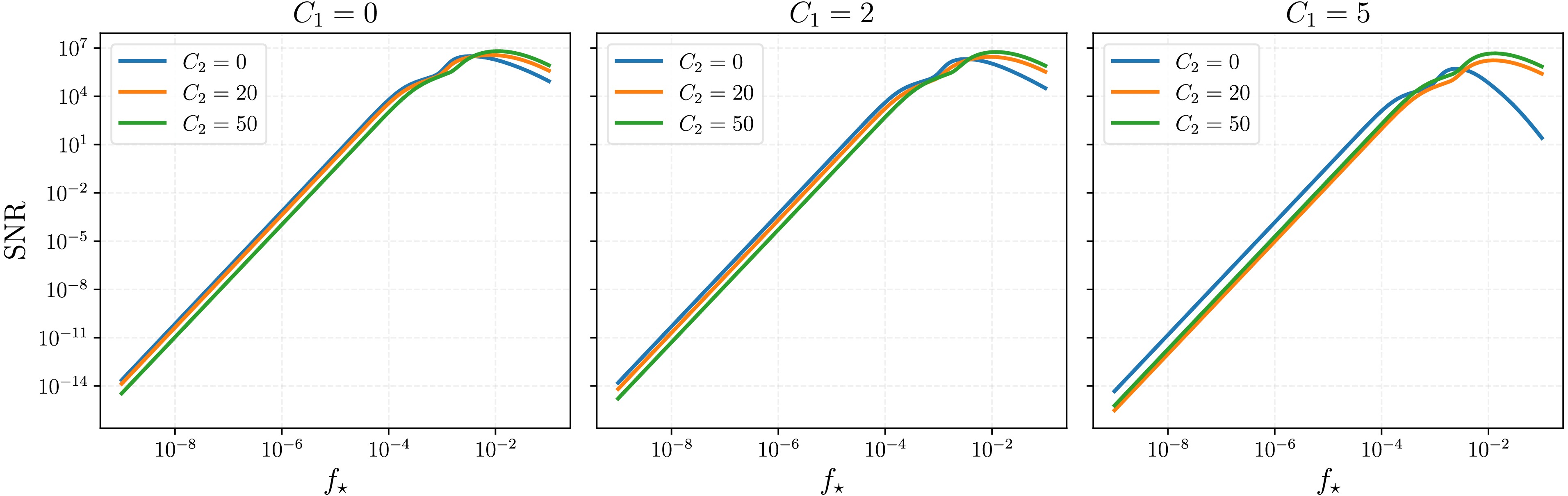
Figure 11. (color online) The SNR of LISA as a function of
$ f_* $ with different$ C_1 $ and$ C_2 $ , calculated for fixed values of$ A_\zeta = 10^{-0.6} $ and$ \sigma = 1 $ . The gray bands represent the 1-σ range from the posterior of$ f_* $ shown in Fig. 5.Furthermore, the gray region in Fig. 5 corresponds to the 1-σ range of the posterior of
$ f_* $ when SIGWs dominate current PTA observations. When$ f_* $ lies within this gray region, regardless of the values of$ C_1 $ and$ C_2 $ , the SNR of LISA does not exceed$ 10^{-2} $ . Therefore, the SIGWs generated by the primordial power spectrum under consideration cannot simultaneously dominate PTA observations and produce a significant impact on the SGWB in the LISA band. This behavior is markedly different from the SGWB produced by SMBHB. When the SMBHB model dominates the PTA signal, the corresponding energy density spectrum can still be detected by LISA [70]. Combining SGWB observations across different frequency bands to jointly constrain or determine various SGWB models and their corresponding parameter spaces may serve as an important tool in the future for distinguishing between different sources of the SGWB.From the above discussion, we find that current cosmological observations are insufficient to place strong constraints on the small-scale anisotropic primordial power spectrum. More precise future observations, combined with SGWB measurements at other frequency bands, will be required to better constrain or determine the properties of the small-scale anisotropic primordial power spectrum. It should be noted that the small-scale anisotropic primordial power spectra considered here are given in parameterized form, in which the anisotropy parameter
$ C_l $ is not subject to any restriction. However, in specific inflationary models, the anisotropy parameters are generally dictated by the intrinsic features of the model, so the parameter$ C_l $ is not completely free. As an illustration, Ref. [71] considered a system constructed by two scalar fields, specifically, an inflaton ϕ and a waterfall field χ, and a vector field$ A_\mu(\mu=0,1,2,3) $ which couples with the waterfall field. The corresponding action can be written as$ \begin{aligned}[b] S=\;&\frac{1}{2} \int {\rm{d}}^4 x \sqrt{-g} R-\int {\rm{d}}^4 x \sqrt{-g}\\&\times\Bigg[\frac{1}{2} g^{\mu \nu}\left(\partial_\mu \phi \partial_\nu \phi+\partial_\mu \chi \partial_\nu \chi\right)+V\left(\phi, \chi, A_\mu\right)\Bigg] \\ &-\frac{1}{4} \int {\rm{d}}^4 x \sqrt{-g} g^{\mu \nu} g^{\rho \sigma} f^2(\phi) F_{\mu \rho} F_{\nu \sigma} \ , \end{aligned} $
(46) where
$ F_{\mu \nu} \equiv \partial_\mu A_\nu-\partial_\nu A_\mu $ is the field strength of the vector field, and an arbitrary function$ f(\phi) $ represents gauge coupling. The potential of field$ V\left(\phi, \chi, A_\mu\right) $ is given by$ V\left(\phi, \chi, A^i\right)=\frac{\lambda}{4}\left(\chi^2-v^2\right)^2+\frac{1}{2} g^2 \phi^2 \chi^2+\frac{1}{2} m^2 \phi^2+\frac{1}{2} h^2 A^\mu A_\mu \chi^2 \ . $
(47) In such a scenario, the anisotropic primordial power spectrum can be represented as
$ {\cal{P}}^{\hat{{\bf{n}}}}_\zeta({\bf{k}}) = {\cal{P}}_{0,\zeta}(k)\left(1-g_*\left(\hat{{\bf{n}}}\cdot\hat{{\bf{k}}}\right)^2\right) \ , $
(48) where
$ g_*=\frac{\beta}{1+\beta} \ , \ \beta \approx \frac{1}{f_e^2}\left(\frac{h^2|{\bf{A}}|}{g^2 \phi_e}\right)^2 \ . $
(49) In this model,
$ g_* $ serves as the parameter quantifying anisotropy. When$ \beta\gg 1 $ ,$ g_*\approx 1 $ , whereas when$ \beta\ll 1 $ ,$ g_*\approx\beta\ll 1 $ . In this case, regardless of how the model parameters vary, it is impossible to generate a very large anisotropic primordial power spectrum. The above example illustrates that, in addition to the constraints from cosmological observations, specific anisotropic inflationary models may impose further restrictions on the anisotropy parameters. For a given model, current cosmological data can be combined with the properties of the model to jointly constrain the parameter space of the small-scale anisotropic primordial power spectrum. -
In Sec. IV.A, we investigate the impact of second-order SIGWs, generated by small-scale anisotropic primordial power spectra, on current PTA observations. By combining PTA data with large-scale cosmological observations, we constrain the small-scale anisotropy parameters. Our results show that when considering a general parameterized form of the anisotropic primordial power spectrum, the presence of anisotropy parameters leads to a certain degree of degeneracy in the energy density spectrum of SIGWs. Consequently, current cosmological observations cannot impose stringent constraints on small-scale anisotropy parameters. To address this issue, we can jointly constrain or determine the parameter space of the small-scale primordial power spectrum by combining SGWB observations at different frequency bands.
As shown by the posterior distributions in Fig. 5, when second-order SIGWs dominate current PTA observations, the parameters
$ A_{\zeta} $ , σ, and$ f_* $ of the isotropic primordial power spectrum$ {\cal{P}}_{0,\zeta} $ can be constrained relatively effectively. However, the anisotropy parameters$ C_1 $ and$ C_2 $ remain unconstrained. In this analysis, we fix the isotropic parameters of$ {\cal{P}}_{0,\zeta} $ to the median values determined by PTA observations (Fig. 5) and vary the anisotropy parameters$ C_1 $ and$ C_2 $ to examine their impact on SGWB observations in the LISA frequency band. More precisely, to asssess the impact of the anisotropic primordial power spectrum on second-order SIGWs, we calculate the signal-to-noise ratio (SNR) ρ for LISA [65–66]:$ \rho = \sqrt{T}\left[ \int {\rm{d}} f\left(\frac{\bar{\Omega}_{{\rm{GW}},0}(f)}{\Omega_{\rm{n}}(f)}\right)^2\right]^{1/2} \ , $
(45) where T is the observation time, and we set
$ T=4 $ years here.$ \Omega_{\rm{n}}(f)=2\pi^2f^3S_n/3H_0^2 $ , where$ H_0 $ is the Hubble constant, and$ S_n $ is the strain noise power spectral density [66]. As illustrated in Fig. 5, if the second-order SIGWs generated by an anisotropic primordial power spectrum dominate the current PTA observations, then$ f_*\approx 10^{-6.7} $ Hz,$ A_{\zeta}\approx 10^{-0.6} $ , and$ \sigma\approx 1.2 $ . In Fig. 11, we present the SNRs of LISA corresponding to different anisotropy parameters$ C_1 $ and$ C_2 $ under this scenario. As shown in Fig. 11, the SNR of LISA increases with the peak position$ f_* $ of the primordial power spectrum. When$ f_*>10^{-3} $ , the anisotropy parameters$ C_1 $ and$ C_2 $ significantly influence the SNR of LISA. Thus, future observations of the SGWB in the LISA frequency band may provide a new window for studying anisotropic inflation models at small scales.
Figure 11. (color online) The SNR of LISA as a function of
$ f_* $ with different$ C_1 $ and$ C_2 $ , calculated for fixed values of$ A_\zeta = 10^{-0.6} $ and$ \sigma = 1 $ . The gray bands represent the 1-σ range from the posterior of$ f_* $ shown in Fig. 5.Furthermore, the gray region in Fig. 5 corresponds to the 1-σ range of the posterior of
$ f_* $ when SIGWs dominate current PTA observations. When$ f_* $ lies within this gray region, irrespective of the values of$ C_1 $ and$ C_2 $ , the SNR of LISA does not exceed$ 10^{-2} $ . Therefore, the SIGWs generated by the primordial power spectrum under consideration cannot simultaneously dominate PTA observations and significantly influence the SGWB in the LISA band. This behavior is markedly different from that of the SGWB produced by SMBHB. When the SMBHB model dominates the PTA signal, the corresponding energy density spectrum can still be detected by LISA [67]. Combining SGWB observations across different frequency bands to jointly constrain or determine various SGWB models and their corresponding parameter spaces may serve as an important tool in the future for distinguishing between different sources of the SGWB.The aforementioned discussion reveals that current cosmological observations are insufficient to impose strong constraints on the small-scale anisotropic primordial power spectrum. More precise future observations, combined with SGWB measurements at other frequency bands, are required to better constrain or determine the properties of the small-scale anisotropic primordial power spectrum. Notably, the small-scale anisotropic primordial power spectra considered here are given in a parameterized form, in which the anisotropy parameter
$ C_l $ is not subject to any restriction. However, in specific inflationary models, the anisotropy parameters are generally dictated by the intrinsic features of the model; thus, the parameter$ C_l $ is not completely free. As an illustration, Yokoyama and Soda [68] considered a system constructed by two scalar fields, specifically, an inflaton ϕ and a waterfall field χ, and a vector field$ A_\mu(\mu=0,1,2,3) $ , which coupled with the waterfall field. The corresponding action can be written as$ \begin{aligned}[b] S=\;&\frac{1}{2} \int {\rm{d}}^4 x \sqrt{-g} R-\int {\rm{d}}^4 x \sqrt{-g}\\&\times\Bigg[\frac{1}{2} g^{\mu \nu}\left(\partial_\mu \phi \partial_\nu \phi+\partial_\mu \chi \partial_\nu \chi\right)+V\left(\phi, \chi, A_\mu\right)\Bigg] \\ &-\frac{1}{4} \int {\rm{d}}^4 x \sqrt{-g} g^{\mu \nu} g^{\rho \sigma} f^2(\phi) F_{\mu \rho} F_{\nu \sigma} \ , \end{aligned} $
(46) where
$ F_{\mu \nu} \equiv \partial_\mu A_\nu-\partial_\nu A_\mu $ is the field strength of the vector field, and an arbitrary function$ f(\phi) $ represents gauge coupling. The potential of field$ V\left(\phi, \chi, A_\mu\right) $ is given by$ V\left(\phi, \chi, A^i\right)=\frac{\lambda}{4}\left(\chi^2-v^2\right)^2+\frac{1}{2} g^2 \phi^2 \chi^2+\frac{1}{2} m^2 \phi^2+\frac{1}{2} h^2 A^\mu A_\mu \chi^2 \ . $
(47) In such a scenario, the anisotropic primordial power spectrum can be represented as
$ {\cal{P}}^{\hat{{\bf{n}}}}_\zeta({\bf{k}}) = {\cal{P}}_{0,\zeta}(k)\left(1-g_*\left(\hat{{\bf{n}}}\cdot\hat{{\bf{k}}}\right)^2\right) \ , $
(48) where
$ g_*=\frac{\beta}{1+\beta} \ , \ \beta \approx \frac{1}{f_e^2}\left(\frac{h^2|{\bf{A}}|}{g^2 \phi_e}\right)^2 \ . $
(49) In this model,
$ g_* $ serves as the parameter quantifying anisotropy. When$ \beta\gg 1 $ ,$ g_*\approx 1 $ , whereas when$ \beta\ll 1 $ ,$ g_*\approx\beta\ll 1 $ . In this case, irrespective of how the model parameters vary, generating an extremely large anisotropic primordial power spectrum is impossible. The above example illustrates that in addition to the constraints from cosmological observations, specific anisotropic inflationary models may impose further restrictions on the anisotropy parameters. For a given model, current cosmological data can be combined with the properties of the model to jointly constrain the parameter space of the small-scale anisotropic primordial power spectrum. -
In this study, we explored the effect of small-scale anisotropic primordial power spectra on the energy density spectrum of second-order SIGWs. In Sec. III, we derive the expression for the energy density spectrum of these waves under the influence of an anisotropic primordial power spectrum. This result is applicable to any form of small-scale anisotropic primordial power spectrum with
$ l \leq 4 $ and remains independent of specific inflation models. As examples, we examine the gauge field and Finslerian inflation models, which correspond to the primordial power spectra with$ C_2\neq 0 $ and$ C_1\neq 0 $ , respectively. We investigate the impact of these two inflation models on current PTA observations and SNR of LISA, and extend the findings to a general scenario, wherein both$ C_1 $ and$ C_2 $ are non-zero.In Sec. IV, we discuss the constraints imposed by current PTA+CMB+BAO data on the small-scale anisotropic primordial power spectrum. Specifically, under the assumption that second-order SIGWs dominate current PTA observations, we analyze the constraints imposed by PTA data on small-scale anisotropic inflation models. To better constrain the parameter space of different models, we incorporate large-scale cosmological observations and present the resulting constraints on the parameter space of the small-scale anisotropic primordial power spectrum in Figs. 7–9. In addition, we examine the feasibility of SIGWs, generated by different small-scale anisotropic inflation models, dominating current PTA signals. The results indicate that current cosmological data can only partially constrain the parameter space of these models, without definitively confirming or ruling them out.
Because current cosmological observations cannot effectively constrain the general form of the anisotropic primordial power spectrum, we further consider the restrictions from future SGWB observations in the LISA frequency band, as well as from specific inflationary models. Using the isotropic primordial power spectrum parameters determined by PTA observations, we analyze the impact of anisotropy parameters
$ C_1 $ and$ C_2 $ on the SNR of LISA under the scenario, wherein SIGWs dominate current PTA observations. The results show that the SIGWs generated by the primordial power spectrum under consideration cannot simultaneously dominate PTA observations and significantly impact the SGWB in the LISA band. Furthermore, we briefly analyze anisotropic primordial power spectra generated by specific models, noting that in certain anisotropic inflationary scenarios, the models themselves impose relatively strict constraints on the anisotropy parameters. -
In this study, we explored how small-scale anisotropic primordial power spectra affect the energy density spectrum of second-order SIGWs. In Sec. III, we derived the expression for the energy density spectrum of these waves under the influence of an anisotropic primordial power spectrum. This result is applicable to any form of small-scale anisotropic primordial power spectrum with
$ l \leq 4 $ and remains independent of specific inflation models. As examples, we examined the gauge field inflation model and the Finslerian inflation model, which correspond to the primordial power spectra with$ C_2\neq 0 $ and$ C_1\neq 0 $ , respectively. We investigated the impact of these two inflation models on current PTA observations and SNR of LISA, and extended the findings to a general scenario where both$ C_1 $ and$ C_2 $ are non-zero.In Sec. IV, we discussed the constraints imposed by current PTA+CMB+BAO data on the small-scale anisotropic primordial power spectrum. Specifically, under the assumption that second-order SIGWs dominate current PTA observations, we analyzed the constraints imposed by PTA data on small-scale anisotropic inflation models. To better constrain the parameter space of different models, we incorporated large-scale cosmological observations and presented the resulting constraints on the parameter space of the small-scale anisotropic primordial power spectrum in Fig. 7–Fig. 9. In addition, we examined the feasibility that SIGWs generated by different small-scale anisotropic inflation models dominate current PTA signals. The results indicate that current cosmological data can only partially constrain the parameter space of these models, without definitively confirming or ruling them out.
Since current cosmological observations cannot effectively constrain the general form of the anisotropic primordial power spectrum, we have further considered the restrictions from future SGWB observations in the LISA frequency band, as well as from specific inflationary models. Using the isotropic primordial power spectrum parameters determined by PTA observations, we analyzed the impact of anisotropy parameters
$ C_1 $ and$ C_2 $ on the SNR of LISA under the scenario where SIGWs dominate current PTA observations. The results show that the SIGWs generated by the primordial power spectrum under consideration cannot simultaneously dominate PTA observations and produce a significant impact on the SGWB in the LISA band. Furthermore, we briefly analyzed anisotropic primordial power spectra generated by specific models, noting that in certain anisotropic inflationary scenarios, the models themselves impose relatively strict constraints on the anisotropy parameters.
Probing small-scale anisotropic inflation with stochastic gravitational-wave background
- Received Date: 2025-10-30
- Available Online: 2026-05-15
Abstract: In June 2023, multiple pulsar timing array (PTA) collaborations provided evidence for the existence of a stochastic gravitational-wave background (SGWB). As a significant source of the SGWB, scalar-induced gravitational waves (SIGWs) receive extensive attention. We explore the influence of anisotropic primordial power spectra on second-order SIGWs and derive explicit expressions for the energy density spectra. For specific anisotropic inflation models, we analyze the impact of Finslerian inflation and gauge field inflation models on PTAs and the Laser Interferometer Space Antenna and generalize the findings to model-independent scenarios. Our results indicate that current PTA observations cannot rule out the existence of small-scale anisotropic primordial perturbations.


 DownLoad: