Schwinger effect in a twice anisotropic holographic model

In high-energy physics, heavy-ion collisions (HIC) conducted at facilities such as the Relativistic Heavy Ion Collider (RHIC) and Large Hadron Collider (LHC) offer a unique opportunity to study physical phenomena under extreme conditions. These experiments are designed to create and investigate the quark-gluon plasma (QGP), a strongly coupled fluid composed of deconfined quarks and gluons [1, 2]. Within this extreme physical environment, one particularly compelling non-perturbative phenomenon is the Schwinger effect: the production of particle-antiparticle pairs from the quantum vacuum under a strong external electromagnetic field. The intense electromagnetic fields generated in HIC provide a promising environment for its observation, making the study of this effect crucial for understanding particle production mechanisms and the quantum structure of the vacuum.

Anti-de Sitter/conformal field theory (AdS/CFT) correspondence provides a natural framework for studying Schwinger pair production at strong coupling [3−5]. In the holographic context, the Schwinger effect was first formulated for $ {\cal{N}} = 4 $ super-Yang Mills (SYM) theory by Semenoff and Zarembo and has since been extended to many gravitational backgrounds [6]. The Schwinger effect in a confining phase was analyzed by Sato and Yoshida through a potential analysis of the corresponding holographic D3-brane and D4-brane backgrounds [7]. The influence of higher-derivative Gauss-Bonnet terms on the holographic Schwinger effect was studied in a confining AdS soliton background [8]. A holographic calculation of the rate of vacuum decay due to the Schwinger effect in confining gauge theories was presented in [9]. [10] investigated the Schwinger effect in a strongly coupled plasma, focusing on the influence of a moving D3-brane and analyzing test particle pair production for motion both transverse and parallel to the plasma wind. The influence of black hole spin on the potential barrier for Schwinger pair production was investigated holographically in Myers-Perry spacetime in [11]. The combined effects of higher derivative corrections and a string cloud background on the holographic Schwinger effect were investigated across both confined and deconfined phases in [12]. Relevant and insightful works can be found in [13−35].

Off-central HIC create extreme early time conditions due to the rapid, oppositely directed motion of the colliding nuclei, which in turn produces strong transient magnetic fields ($ 10^{-1} \cdot m_\pi^2\sim 15 \cdot m_\pi^2 $) [36, 37]. Concurrently, experimental data from HIC indicate an early stage local anisotropy in the QGP, as the system expands predominantly along the collision axis and this anisotropy lasts for several fm/c [38, 39]. The presence of these anisotropies in realistic HIC scenarios motivates investigations of the Schwinger effect within various anisotropic holographic models to capture these characteristics. Previous studies have typically examined the influence of a single source of anisotropy, either spatial or magnetic, on the holographic Schwinger effect. In [30], the authors employed a top-down holographic approach to systematically analyze the Schwinger effect and associated electric instabilities in the dual anisotropic gauge theory. [40] investigated the holographic Schwinger effect in an anisotropic background and found that anisotropy suppresses pair production compared to that in the isotropic case. [32] systematically analyzed the holographic Schwinger effect in the presence of weak and strong magnetic fields at RHIC and LHC energies and demonstrated that magnetic fields reduce the potential barrier to favor pair creation. To simultaneously capture the spatial and magnetic anisotropies observed in realistic HIC, this work employs a five-dimensional Einstein-Maxwell-Dilaton model with three Maxwell fields. The Schwinger effect is investigated within this twice anisotropic holographic model by calculating the total potential of a particle pair.

The remainder of this paper is organized as follows. Sec. II briefly reviews the anisotropic holographic model used in this study. Sec. III presents the detailed potential analysis for the Schwinger effect and our numerical results. Finally, Sec. IV summarizes our findings and discusses potential extensions.

In this section, we briefly review the anisotropic holographic QCD model introduced in [41−44], which has been used to study hot dense anisotropic QCD in the presence of an external magnetic field. The five-dimensional Einstein-Maxwell-dilaton gravity action with three Maxwell fields is given by

In this model, the first ($ F_0 $), second ($ F_1 $), and third ($ F_3 $) Maxwell fields are responsible for establishing a finite chemical potential, inducing spatial anisotropy, and providing an additional anisotropy sourced by the magnetic field, respectively. Following [43], the holographic anisotropic background is described by a metric ansatz of the form

In this framework, z is the holographic radial coordinate, L is the AdS radius (set to one), $ \mathfrak{b}(z) $ is the AdS deformation factor, $ g(z) $ is the blackening function, ν is the anisotropy parameter characterizing primary spatial anisotropy, $ c_B $ is the magnetic coefficient of secondary anisotropy induced by a magnetic field in the $ x_3 $ direction, and $ q_1 $ and $ q_3 $ are constant charges. Here, $ q_3 $ quantifies the magnitude of the magnetic field source, while $ c_B $ governs the magnetic field's back-reaction on the geometry [41−44].

We adopt $ { \cal{A}}(z) = - \, cz^2/4 \, - (p - c_B q_3) z^4 $, with the parameters $ c = 4 R_{gg}/3 $, $ R_{gg} = 1.16 $, and $ p = 0.273 $, to reproduce specific QCD phenomena [45]. In accordance with [43], solving the equations of motion yields the following expressions for the blackening function:

μ denotes the chemical potential, which is holographically identified with the boundary value of the temporal component of the gauge field. Accordingly, the Hawking temperature and entropy can be written as follows:

where $ z_h $ is the black hole horizon.

Because the $ x_1 $ and $ x_2 $ directions can be considered simplified special cases of the $ x_3 $ direction when $ c_B=0 $ and $ \nu=1 $, in the following, we take the $ x_3 $ direction as an explicit example for the derivation by aligning both the particle pair and external electric field along the $ x_3 $ direction. The coordinates are parameterized by

Derived from the classical string action, the Nambu-Goto action is

where $ T_{F} $ represents the string tension, and $ {\rm{det}} g_{\alpha \beta} $ is the determinant of the induced metric on the string worldsheet. The Lagrangian density derived from the Nambu-Goto action is given as

Because the action is independent of the worldsheet coordinate σ, the associated Hamiltonian is conserved and given by

Under the boundary condition

wherein the probe D3-brane is located at the radial coordinate $ z_{0} $, one obtains the differential equation

Integration of Eq. (13) directly provides the separation length x for the test particle pair, which is expressed as

Calculation of the combined Coulomb potential and static energy is performed according to

The critical electric field, $ E_c $, is determined from the Dirac-Born-Infeld (DBI) action, given by

Requiring the $S_{\rm DBI}$ action to be free of singularities determines the critical field $ E_c $:

By defining the dimensionless parameter $ \alpha \equiv \dfrac{E}{E_{c}} $, the total potential $V_{\rm tot}$ of the pair can be formulated as

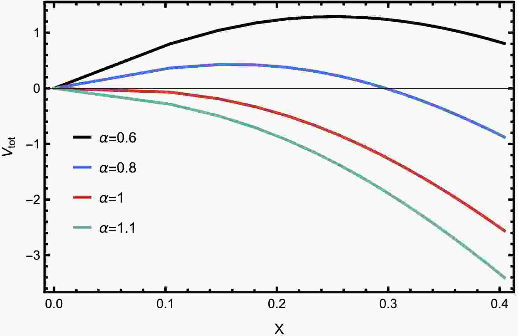
The calculation for the $ x_1 $ direction (perpendicular to the magnetic field) is analogous to that for the $ x_3 $ direction (parallel to the magnetic field). Within this framework, we investigate the Schwinger effect in the presence of two sources of anisotropy, one originating from spatial anisotropy and the other from an external magnetic field. Considering the numerical results, we refer to Fig. 1, which shows how the total potential $V_{\rm tot}$ varies with separation length x for various electric field strengths at $T= 0.6\ \rm GeV$.

Figure 1.  (color online) Total potential $V_{\rm tot}$ as a function of separation length x for various electric field strengths at $ c_B = - \, 0.1 $, $ \nu = 1.1 $, $ q_3 = 1 $, $ \mu = 0.1 $, and $ T= 0.6 $.

Observations indicate that the external electric field strength critically influences the rate of Schwinger pair production. The potential barrier diminishes with increasing field strength and disappears at the critical point ($ \alpha = 1 $). When $ \alpha \lt 1 $, pair production occurs via quantum tunneling through the barrier. For $ \alpha \gt 1 $, the suppression is removed and pair production becomes explosive, leading to vacuum instability. The influence of the magnetic field on the Schwinger effect is characterized by evaluating the total potential $V_{\rm tot}$ versus separation length x over ranges of the magnetic coefficient $ c_B $ and magnetic charge $ q_3 $. Figure 2 illustrates the impact of magnetic charge $ q_3 $ on the potential barrier by plotting the total potential against the separation distance with α fixed at 0.8.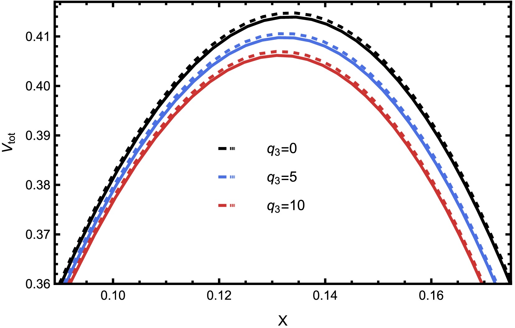

Figure 2.  (color online) Total potential $V_{\rm tot}$ as a function of separation length x for various magnetic charges $ q_3 $ at $ c_B = - \, 0.1 $, $ \nu = 1.1 $, $ \mu = 0.1 $, and $ T= 0.6 $. The solid (dashed) line corresponds to the case where the particle pair and external electric field are parallel (perpendicular) to the magnetic field.

As shown in Fig. 2, an increase in magnetic charge reduces both the height and width of the potential barrier, thereby increasing the tunneling probability of virtual particle–antiparticle pairs and consequently enhancing the Schwinger effect. To reveal the effect of the magnetic coefficient, Fig. 3 presents the total potential versus separation distance, wherein we increase the absolute magnitude of the magnetic coefficient $ c_B $ while maintaining a fixed magnetic charge.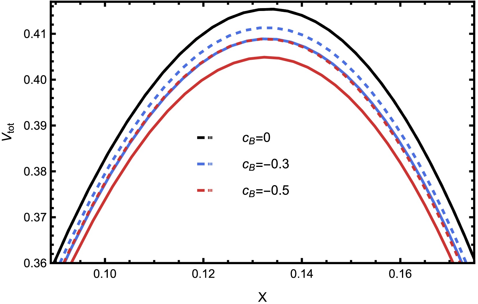

Figure 3.  (color online) Total potential $V_{\rm tot}$ as a function of separation length x for various magnetic coefficients $ c_B $ at $ \nu = 1.1 $, $ q_3 = 1 $, $ \mu = 0.1 $, and $ T= 0.6 $. The solid (dashed) line corresponds to the case where the particle pair and external electric field are parallel (perpendicular) to the magnetic field.

As depicted in Fig. 3, the height and width of the potential barrier diminish with increasing absolute magnitude of the magnetic coefficient $ c_B $, which in turn facilitates the Schwinger effect.

Collectively, these findings underscore that the potential barrier is significantly influenced by both magnetic field parameters, namely the magnetic coefficient $ c_B $ and magnetic charge $ q_3 $. As revealed in Fig. 2 and Fig. 3, increasing the absolute values of the magnetic parameters $ c_B $ and $ q_3 $ consistently lowers and narrows the potential barrier. This directly translates to an enhanced Schwinger effect, indicating that stronger magnetic fields facilitate pair production. It is also observed that the Schwinger effect is more pronounced in the parallel case. This is because the magnetic field dependence enters the metric mainly in the $ x_3 $ component, thereby lowering the potential barrier more effectively in the parallel case than in the transverse case. These results from the potential analyses are in qualitative agreement with the results presented in [32, 33].

Turning to the influence of spatial anisotropy, parametrized by ν, the potential barrier is also noticeably affected. Here, we focus on the $ x_3 $ direction, as the $ x_1 $ metric component contains no explicit ν dependence. Figure 4 examines the role of spatial anisotropy in the Schwinger effect by plotting the total potential $V_{\rm tot}$ versus separation distance x across varying anisotropy parameter ν, with all magnetic parameters fixed.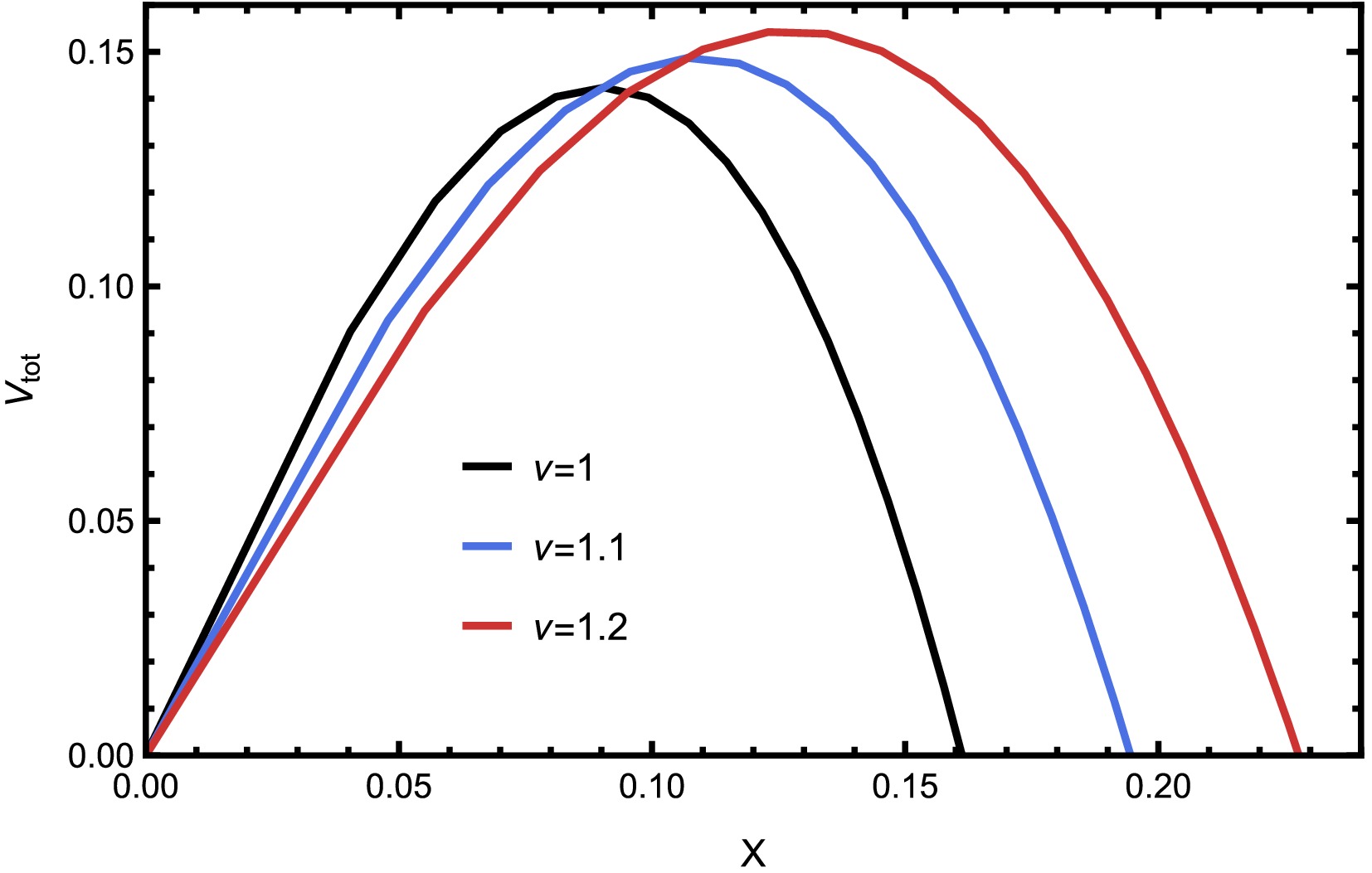

Figure 4.  (color online) Total potential $V_{\rm tot}$ as a function of separation length x for various anisotropy parameter ν at $ c_B = - \, 0.1 $, $ q_3 = 1 $, $ \mu = 0.1 $, and $ T= 0.6 $.

In contrast to magnetic parameters that reduce the barrier, Fig. 4 indicates that, as ν increases, corresponding to greater spatial anisotropy, the potential barrier’s height and width both expand significantly. In turn, this suppresses the pair production process, thereby weakening the Schwinger effect, which is consistent with the calculations presented in [40].

In this work, we investigated the Schwinger effect within an anisotropic holographic QCD model, focusing on the influence of two distinct sources of anisotropy: spatial anisotropy (parameterized by ν) and external magnetic field (characterized by the magnetic coefficient $ c_B $ and magnetic charge $ q_3 $). By utilizing the AdS/CFT correspondence, we calculated the total potential of the particle pair and analyzed the behavior of the potential barrier that governs the pair production phenomenon under the influence of these anisotropic parameters. We first summarize our numerical findings and their physical implications, and then we discuss potential extensions for future work.

The influence of the magnetic field parameters, $ c_B $ and $ q_3 $, was found to consistently enhance the Schwinger effect. As demonstrated in Fig. 2 and Fig. 3, increasing the magnetic charge $ q_3 $ or the absolute magnitude of the magnetic coefficient $ c_B $ leads to a reduction in both the height and width of the potential barrier, thereby promoting the Schwinger effect. These findings are in qualitative agreement with previous studies [32, 33] and suggest that stronger magnetic environments facilitate pair production. In contrast to the magnetic case, increasing the spatial anisotropy, characterized by the parameter ν, results in a significant increase in both the height and width of the potential barrier, consequently weakening the Schwinger effect, which aligns with earlier findings [40]. Physically, this behavior arises because a stronger magnetic field reduces the string tension, thereby facilitating pair separation, whereas spatial anisotropy counteracts this effect [46, 47].

In realistic HIC, both the magnetic field and spatial anisotropy evolve rapidly in time. A natural extension would be to generalize our analysis to a time-dependent holographic background that incorporates the evolution of both of these effects.