


 Abstract
 HTML
HTML Reference
 Related
 PDF
PDF


-
Experimental research conducted at the Relativistic Heavy Ion Collider (RHIC) and Large Hadron Collider (LHC) enables the exploration of quantum chromodynamics (QCD) matter in extreme environments [1−4]. These heavy-ion collisions experiments produce an extremely hot and dense environment, leading to the formation of the strongly coupled quark-gluon plasma (QGP). Heavy quarkonium serve as essential probes for examining QGP properties and offer insights into the behavior of strongly interacting matter. The suppression of heavy quarkonium can be considered as the signal of the in-medium interaction and has attracted research interest [5, 6]. The thermal dissociation of heavy quarkonia manifests as the disappearance of the bound state peak from the spectral function.
Lattice QCD encounters significant challenges in studying regions with finite chemical potential because of the sign problem. The AdS/CFT correspondence [7−9] has been extensively employed as a non-perturbative approach to investigate strongly interacting matter under extreme conditions [10−22]. The AdS/CFT correspondence also serves as an effective approach for investigating heavy quarkonium dissociation. Holographic studies have examined the melting of scalar glueballs and mesons at finite temperature [23, 24], as well as the impact of magnetic fields on the quarkonium [25−28]. The effects of temperature and chemical potential on the dissociation have been analyzed [29−33]. The masses and decay constants of heavy quarkonium states have also been discussed [34, 35]. Further investigations include quasinormal modes [36, 37], spectral functions in rotating systems [38−40], and anisotropy effects [41] on quarkonium behavior. The dynamical holographic QCD model has been used to study light-flavor hadron spectra [42], and vector meson dilepton decay rates have been linked to spectral functions [43]. Other studies have focused on
$ J/\Psi $ spectral functions in the soft wall model [44] and meson dissociation in two-flavor scenarios [45].In this work, we investigate the dissociation of heavy quarkonium from a data-driven holographic QCD model. Recently, machine learning has emerged as a valuable tool. Unlike traditional holographic methods, the strategy of machine learning is to use QCD data to infer the bulk metric and other model parameters via machine learning. Recent studies have integrated machine learning with holographic QCD [46−57]. Using machine-learning techniques, the authors of [55, 56] determined the black hole metric in the Einstein-Maxwell-Dilaton (EMD) model based on lattice equation of state data for 2+1-flavor QCD at zero chemical potential.
While the foundational EMD framework and machine-learning strategy for parameter determination are adopted from Refs. [55, 56], the specific form of the dilaton field used in our spectral function calculation is taken from Ref. [26]. This choice is motivated by the fact that the dilaton profile in [26] was particularly designed and successfully tested for describing the properties of heavy quarkonium states.
The data-driven EMD background ensures a bulk geometry consistent with QCD thermodynamics, whereas the dilaton profile from [26] is specifically selected because it has been shown to successfully describe the properties of heavy quarkonium states. We combine a data-driven gravitational background with a distinct dilaton profile proven specifically for heavy quarkonium. This ensures precision for both the hot medium and embedded probe. We systematically investigate quarkonium dissociation in a holographic framework that is firmly grounded in QCD data, particularly extending the analysis to finite baryon chemical potential where lattice QCD encounters challenges.
The remainder of this paper is organized as follows. In Sec. II, we briefly review the holographic model through machine learning. In Sec. III, we discuss the spectral function from holographic QCD through machine learning. In Sec. IV, we present the conclusion and discussion.
-
Experimental research conducted at the Relativistic Heavy Ion Collider (RHIC) and the Large Hadron Collider (LHC) enables the exploration of quantum chromodynamics (QCD) matter in extreme environments [1−4]. These heavy-ion collisions experiments produce an extremely hot and dense environment, leading to the formation of the strongly coupled quark-gluon plasma (QGP). Heavy quarkonium serve as essential probes for examining QGP properties and offer insights into the behavior of strongly interacting matter. The suppression of heavy quarkonium can be seen as the signal of the in-medium interaction and has attracted research attention [5, 6]. The thermal dissociation of heavy quarkonia manifests as the disappearance of the bound state peak from the spectral function.
Lattice QCD faces significant challenges in studying regions with finite chemical potential because of the sign problem. The AdS/CFT correspondence [7−9] has been extensively employed as a non-perturbative approach to investigate strongly interacting matter under extreme conditions [10−22]. The AdS/CFT correspondence also serves as a powerful approach to investigate heavy quarkonium dissociation. Holographic studies have examined the melting of scalar glueballs and mesons at finite temperature [23, 24], as well as the impact of magnetic fields on the quarkonium [25−28]. The effects of temperature and chemical potential on the dissociation have been analyzed in [29−33]. The masses and decay constants of heavy quarkonium states have also been discussed [34, 35]. Further investigations include quasinormal modes [36, 37], spectral functions in rotating systems [38−40], and anisotropy effects [41] on quarkonium behavior. The dynamical holographic QCD model has been used to study light-flavor hadron spectra [42], and vector meson dilepton decay rates have been linked to spectral functions [43]. Additional studies focus on
$ J/\Psi $ spectral functions in the soft wall model [44] and meson dissociation in two-flavor scenarios [45].In this work, we investigate the dissociation of heavy quarkonium from a data-driven holographic QCD model. Recent years, the machine learning has emerged as a valuable tool. Unlike traditional holographic methods, the strategy of machine learning is to use QCD data to infer the bulk metric and other model parameters via machine learning. Recent studies have integrated machine learning with holographic QCD [46−57]. By using the machine learning techniques, the authors of [55, 56] determine the black hole metric in the Einstein-Maxwell-Dilaton (EMD) model based on lattice equation of state (EOS) data for 2+1-flavor QCD at zero chemical potential.
While the foundational Einstein-Maxwell-Dilaton (EMD) framework and the machine-learning strategy for parameters determination are adopted from Refs.[55, 56], the specific form of the dilaton field used in our spectral function calculation is taken from Ref [26]. This choice is motivated by the fact that the dilaton profile in [26] was particularly designed and successfully tested for describing the properties of heavy quarkonium states.
The data-driven EMD background ensures a bulk geometry consistent with QCD thermodynamics, while the dilaton profile from [26] is specifically chosen because it has been shown to successfully describe the properties of heavy quarkonium states. We combine a data-driven gravitational background with a distinct dilaton profile proven specifically for heavy quarkonium. This ensures precision for both the hot medium and the embedded probe. We systematically investigate quarkonium dissociation in a holographic framework that is firmly grounded in QCD data, particularly extending the analysis to finite baryon chemical potential where lattice QCD face challenges.
The paper is organized as follows. In Sec. II, we briefly review the holographic model through machine learning. In Sec. III, we discuss the spectral function from holographic QCD through machine learning. In Sec. IV, we give the conclusion and discussion.
-
Experimental research conducted at the Relativistic Heavy Ion Collider (RHIC) and Large Hadron Collider (LHC) enables the exploration of quantum chromodynamics (QCD) matter in extreme environments [1−4]. These heavy-ion collisions experiments produce an extremely hot and dense environment, leading to the formation of the strongly coupled quark-gluon plasma (QGP). Heavy quarkonium serve as essential probes for examining QGP properties and offer insights into the behavior of strongly interacting matter. The suppression of heavy quarkonium can be considered as the signal of the in-medium interaction and has attracted research interest [5, 6]. The thermal dissociation of heavy quarkonia manifests as the disappearance of the bound state peak from the spectral function.
Lattice QCD encounters significant challenges in studying regions with finite chemical potential because of the sign problem. The AdS/CFT correspondence [7−9] has been extensively employed as a non-perturbative approach to investigate strongly interacting matter under extreme conditions [10−22]. The AdS/CFT correspondence also serves as an effective approach for investigating heavy quarkonium dissociation. Holographic studies have examined the melting of scalar glueballs and mesons at finite temperature [23, 24], as well as the impact of magnetic fields on the quarkonium [25−28]. The effects of temperature and chemical potential on the dissociation have been analyzed [29−33]. The masses and decay constants of heavy quarkonium states have also been discussed [34, 35]. Further investigations include quasinormal modes [36, 37], spectral functions in rotating systems [38−40], and anisotropy effects [41] on quarkonium behavior. The dynamical holographic QCD model has been used to study light-flavor hadron spectra [42], and vector meson dilepton decay rates have been linked to spectral functions [43]. Other studies have focused on
$ J/\Psi $ spectral functions in the soft wall model [44] and meson dissociation in two-flavor scenarios [45].In this work, we investigate the dissociation of heavy quarkonium from a data-driven holographic QCD model. Recently, machine learning has emerged as a valuable tool. Unlike traditional holographic methods, the strategy of machine learning is to use QCD data to infer the bulk metric and other model parameters via machine learning. Recent studies have integrated machine learning with holographic QCD [46−57]. Using machine-learning techniques, the authors of [55, 56] determined the black hole metric in the Einstein-Maxwell-Dilaton (EMD) model based on lattice equation of state data for 2+1-flavor QCD at zero chemical potential.
While the foundational EMD framework and machine-learning strategy for parameter determination are adopted from Refs. [55, 56], the specific form of the dilaton field used in our spectral function calculation is taken from Ref. [26]. This choice is motivated by the fact that the dilaton profile in [26] was particularly designed and successfully tested for describing the properties of heavy quarkonium states.
The data-driven EMD background ensures a bulk geometry consistent with QCD thermodynamics, whereas the dilaton profile from [26] is specifically selected because it has been shown to successfully describe the properties of heavy quarkonium states. We combine a data-driven gravitational background with a distinct dilaton profile proven specifically for heavy quarkonium. This ensures precision for both the hot medium and embedded probe. We systematically investigate quarkonium dissociation in a holographic framework that is firmly grounded in QCD data, particularly extending the analysis to finite baryon chemical potential where lattice QCD encounters challenges.
The remainder of this paper is organized as follows. In Sec. II, we briefly review the holographic model through machine learning. In Sec. III, we discuss the spectral function from holographic QCD through machine learning. In Sec. IV, we present the conclusion and discussion.
-
The holographic model used in this study is the data-driven EMD model from Refs. [55, 56]. This section briefly introduces this model and its parameter determination process to establish the foundation for our subsequent calculations. We first review the general EMD systems [12, 13]. The action in Einstein frame is
$ \begin{aligned} S& =\frac{1}{16 \pi G_5} \int {\rm d}^5 x \sqrt{-g}\left[R-\frac{f(\phi_s)}{4} F^2-\frac{1}{2} \partial_\mu \phi_s \partial^\mu \phi_s -V(\phi_s)\right], \\ \end{aligned} $
(1) where the gauge kinetic function
$ f(\phi_s) $ , Maxwell field$ A_\mu $ , and dilaton potential$ V(\phi_s) $ are determined self-consistently from the equations of motion. Here,$ G_5 $ denotes the five-dimensional Newton constant, and$ \phi_s $ is the dilaton field.We can consider the followng ansatz of metric
$ \begin{aligned} {\rm d} s^2=\frac{L^2 {\rm e}^{2 A(z)}}{z^2}\left[-g(z) {\rm d} t^2+\frac{{\rm d} z^2}{g(z)}+ {\rm d} \vec{x}^2\right], \end{aligned} $
(2) where L is the AdS radius, and we set
$ L = 1 $ in the calculations.Using this metric ansatz, the equations of motion and constraints for the background fields are
$ \begin{aligned} \begin{gathered} \phi^{\prime \prime}_s+\phi^{\prime}_s\left(-\frac{3}{z}+\frac{g^{\prime}}{g}+3 A^{\prime}\right)-\frac{ {\rm e}^{2 A}}{z^2 g} \frac{\partial V}{\partial \phi_s}+\frac{z^2 {\rm e}^{-2 A} A_t^{\prime 2}}{2 g} \frac{\partial f}{\partial \phi_s}=0, \end{gathered} \end{aligned} $
(3) $ \begin{aligned} A_t^{\prime \prime}+A_t^{\prime}\left(-\frac{1}{z}+\frac{f^{\prime}}{f}+A^{\prime}\right)=0, \end{aligned} $
(4) $ \begin{aligned} g^{\prime \prime}+g^{\prime}\left(-\frac{3}{z}+3 A^{\prime}\right)- {\rm e}^{-2 A} A_t^{\prime 2} z^2 f=0, \end{aligned} $
(5) $ \begin{aligned}[b] & A^{\prime \prime} +\frac{g^{\prime \prime}}{6 g}+A^{\prime}\left(-\frac{6}{z}+\frac{3 g^{\prime}}{2 g }\right)-\frac{1}{z}\left(-\frac{4}{z}+\frac{3 g^{\prime}}{2 g}\right) \\ & \quad +3 A^{\prime 2}+\frac{ {\rm e}^{2 A} V}{3 z^2 g}=0, \end{aligned} $
(6) $ \begin{aligned} A^{\prime \prime}-A^{\prime}\left(-\frac{2}{z}+A^{\prime}\right)+\frac{\phi^{\prime 2}}{6}=0. \end{aligned} $
(7) We can obtain
$ \begin{aligned}[b] g(z) =\;&1-\frac{1}{\displaystyle\int_0^{z h} {\rm d} x x^3 {\rm e}^{-3 A(x)}}\Big[\int_0^z {\rm d} x x^3 {\rm e}^{-3 A(x)} \\ & +\frac{2 c \mu^2 {\rm e}^k}{\left(1-{\rm e}^{-c z_h^2}\right)^2} \operatorname{det} {\cal{G}}\Big],\\ \phi_s^{\prime}(z) =\;&\sqrt{6\left(A^{\prime 2}-A^{\prime \prime}-2 A^{\prime} / z\right)}, \\ A_t(z) =\;&\mu \frac{{\rm e}^{-c z^2}-{\rm e}^{-c z_h^2}}{1-{\rm e}^{-c z_h^2}}, \\ V(z) =\;&-3 z^2 g {\rm e}^{-2 A}\Big[A^{\prime \prime}+A^{\prime}\left(3 A^{\prime}-\frac{6}{z}+\frac{3 g^{\prime}}{2 g}\right) \\ & -\frac{1}{z}\left(-\frac{4}{z}+\frac{3 g^{\prime}}{2 g}\right)+\frac{g^{\prime \prime}}{6 g}\Big], \end{aligned} $
(8) where
$ \begin{aligned} \operatorname{det} {\cal{G}}=\left|\begin{array}{ll} \displaystyle\int_0^{z_h} {\rm d} y y^3 {\rm e}^{-3 A(y)} & \displaystyle\int_0^{z_h} {\rm d} y y^3 {\rm e}^{-3 A(y)-c y^2} \\ \displaystyle\int_{z_h}^z {\rm d} y y^3 {\rm e}^{-3 A(y)} & \displaystyle\int_{z_h}^z {\rm d} y y^3 {\rm e}^{-3 A(y)-c y^2} \end{array}\right|. \end{aligned} $
(9) The Hawking temperature is
$ \begin{aligned}[b] T =\;&\frac{z_h^3 {\rm e}^{-3 A\left(z_h\right)}}{4 \pi \displaystyle\int_0^{z_h} {\rm d} y y^3 {\rm e}^{-3 A(y)}}\\ &\Bigg[1+ \frac{2 c \mu^2 {\rm e}^k\left({\rm e}^{-c z_h^2} \int_0^{z_h} {\rm d} y y^3 {\rm e}^{-3 A(y)}-\int_0^{z_h} {\rm d} y y^3 {\rm e}^{-3 A(y)} {\rm e}^{-c y^2}\right)}{(1-{\rm e}^{-c z_h^2})^2} \Bigg]. \end{aligned} $
(10) We can take
$ \begin{aligned} A(z)={\rm d} \ln \left(a z^2+1\right)+{\rm d} \ln \left(b z^4+1\right) \text {, } \end{aligned} $
(11) and the gauge kinetic function
$ f(z) $ as [55, 56]$ \begin{aligned} f(z)={\rm e}^{c z^2-A(z)+k}. \end{aligned} $
(12) As studied in [55, 56], the parameters
$ a,b,c,d,k $ fitting for the 2+1 flavor system was accomplished through a machine learning that utilized lattice QCD data as its foundation. The approach utilized 55 entropy measurement points along with 15 baryon number susceptibility values to develop an accurate predictive model. The procedure established a neural network that learned the relationship between temperature and thermodynamic observables through extensive training. Subsequently, the authors of [55, 56] implemented an optimization framework that adjusted the physical parameters by minimizing the discrepancy between the theoretical model's predictions and the neural network's outputs. This process employed the Adam optimization algorithm across 5000 iterations while maintaining physical constraints on parameters, ultimately producing the final optimized parameter set for the 2+1 flavor system. As the results,$ a=0.204, b=0.013, \; c= -0.264, \; d= -0.173, \; k= -0.824, \; G_5=0.400 $ and the critical temperature$ T_c $ is 0.128 GeV.A potential concern is that the temperature dependence of the potential
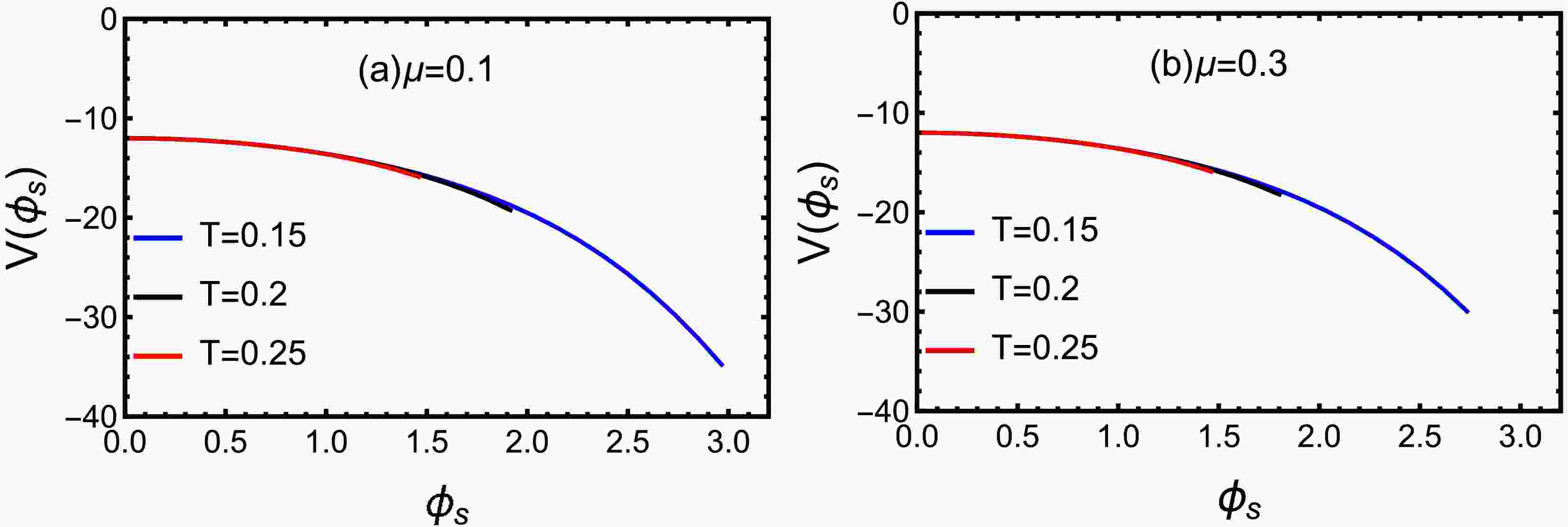
$ V(\phi_s) $ might suggest different temperatures corresponding to different actions. Note that$ V(\phi_s) $ does not explicitly depend on temperature. As illustrated in Fig. 1, the profile of$ V(\phi_s) $ remains nearly identical across different temperatures in regions away from the horizon. Only in the near-horizon region do the curves separate slightly, indicating that the temperature effect is minimal.
Figure 1. (color online) Potential
$ V(\phi_s) $ as a function of dilaton$ \phi_s $ with different values of temperature. μ and T are in units of GeV. -
The holographic model used in this study is the data-driven EMD model from Refs. [55, 56]. This section briefly introduces this model and its parameter determination process to establish the foundation for our subsequent calculations. We first review the general EMD systems [12, 13]. The action in Einstein frame is
$ \begin{aligned} S& =\frac{1}{16 \pi G_5} \int {\rm d}^5 x \sqrt{-g}\left[R-\frac{f(\phi_s)}{4} F^2-\frac{1}{2} \partial_\mu \phi_s \partial^\mu \phi_s -V(\phi_s)\right], \\ \end{aligned} $
(1) where the gauge kinetic function
$ f(\phi_s) $ , Maxwell field$ A_\mu $ , and dilaton potential$ V(\phi_s) $ are determined self-consistently from the equations of motion. Here,$ G_5 $ denotes the five-dimensional Newton constant, and$ \phi_s $ is the dilaton field.We can consider the followng ansatz of metric
$ \begin{aligned} {\rm d} s^2=\frac{L^2 {\rm e}^{2 A(z)}}{z^2}\left[-g(z) {\rm d} t^2+\frac{{\rm d} z^2}{g(z)}+ {\rm d} \vec{x}^2\right], \end{aligned} $
(2) where L is the AdS radius, and we set
$ L = 1 $ in the calculations.Using this metric ansatz, the equations of motion and constraints for the background fields are
$ \begin{aligned} \begin{gathered} \phi^{\prime \prime}_s+\phi^{\prime}_s\left(-\frac{3}{z}+\frac{g^{\prime}}{g}+3 A^{\prime}\right)-\frac{ {\rm e}^{2 A}}{z^2 g} \frac{\partial V}{\partial \phi_s}+\frac{z^2 {\rm e}^{-2 A} A_t^{\prime 2}}{2 g} \frac{\partial f}{\partial \phi_s}=0, \end{gathered} \end{aligned} $
(3) $ \begin{aligned} A_t^{\prime \prime}+A_t^{\prime}\left(-\frac{1}{z}+\frac{f^{\prime}}{f}+A^{\prime}\right)=0, \end{aligned} $
(4) $ \begin{aligned} g^{\prime \prime}+g^{\prime}\left(-\frac{3}{z}+3 A^{\prime}\right)- {\rm e}^{-2 A} A_t^{\prime 2} z^2 f=0, \end{aligned} $
(5) $ \begin{aligned}[b] & A^{\prime \prime} +\frac{g^{\prime \prime}}{6 g}+A^{\prime}\left(-\frac{6}{z}+\frac{3 g^{\prime}}{2 g }\right)-\frac{1}{z}\left(-\frac{4}{z}+\frac{3 g^{\prime}}{2 g}\right) \\ & \quad +3 A^{\prime 2}+\frac{ {\rm e}^{2 A} V}{3 z^2 g}=0, \end{aligned} $
(6) $ \begin{aligned} A^{\prime \prime}-A^{\prime}\left(-\frac{2}{z}+A^{\prime}\right)+\frac{\phi^{\prime 2}}{6}=0. \end{aligned} $
(7) We can obtain
$ \begin{aligned}[b] g(z) =\;&1-\frac{1}{\displaystyle\int_0^{z h} {\rm d} x x^3 {\rm e}^{-3 A(x)}}\Big[\int_0^z {\rm d} x x^3 {\rm e}^{-3 A(x)} \\ & +\frac{2 c \mu^2 {\rm e}^k}{\left(1-{\rm e}^{-c z_h^2}\right)^2} \operatorname{det} {\cal{G}}\Big],\\ \phi_s^{\prime}(z) =\;&\sqrt{6\left(A^{\prime 2}-A^{\prime \prime}-2 A^{\prime} / z\right)}, \\ A_t(z) =\;&\mu \frac{{\rm e}^{-c z^2}-{\rm e}^{-c z_h^2}}{1-{\rm e}^{-c z_h^2}}, \\ V(z) =\;&-3 z^2 g {\rm e}^{-2 A}\Big[A^{\prime \prime}+A^{\prime}\left(3 A^{\prime}-\frac{6}{z}+\frac{3 g^{\prime}}{2 g}\right) \\ & -\frac{1}{z}\left(-\frac{4}{z}+\frac{3 g^{\prime}}{2 g}\right)+\frac{g^{\prime \prime}}{6 g}\Big], \end{aligned} $
(8) where
$ \begin{aligned} \operatorname{det} {\cal{G}}=\left|\begin{array}{ll} \displaystyle\int_0^{z_h} {\rm d} y y^3 {\rm e}^{-3 A(y)} & \displaystyle\int_0^{z_h} {\rm d} y y^3 {\rm e}^{-3 A(y)-c y^2} \\ \displaystyle\int_{z_h}^z {\rm d} y y^3 {\rm e}^{-3 A(y)} & \displaystyle\int_{z_h}^z {\rm d} y y^3 {\rm e}^{-3 A(y)-c y^2} \end{array}\right|. \end{aligned} $
(9) The Hawking temperature is
$ \begin{aligned}[b] T =\;&\frac{z_h^3 {\rm e}^{-3 A\left(z_h\right)}}{4 \pi \displaystyle\int_0^{z_h} {\rm d} y y^3 {\rm e}^{-3 A(y)}}\\ &\Bigg[1+ \frac{2 c \mu^2 {\rm e}^k\left({\rm e}^{-c z_h^2} \int_0^{z_h} {\rm d} y y^3 {\rm e}^{-3 A(y)}-\int_0^{z_h} {\rm d} y y^3 {\rm e}^{-3 A(y)} {\rm e}^{-c y^2}\right)}{(1-{\rm e}^{-c z_h^2})^2} \Bigg]. \end{aligned} $
(10) We can take
$ \begin{aligned} A(z)={\rm d} \ln \left(a z^2+1\right)+{\rm d} \ln \left(b z^4+1\right) \text {, } \end{aligned} $
(11) and the gauge kinetic function
$ f(z) $ as [55, 56]$ \begin{aligned} f(z)={\rm e}^{c z^2-A(z)+k}. \end{aligned} $
(12) As studied in [55, 56], the parameters
$ a,b,c,d,k $ fitting for the 2+1 flavor system was accomplished through a machine learning that utilized lattice QCD data as its foundation. The approach utilized 55 entropy measurement points along with 15 baryon number susceptibility values to develop an accurate predictive model. The procedure established a neural network that learned the relationship between temperature and thermodynamic observables through extensive training. Subsequently, the authors of [55, 56] implemented an optimization framework that adjusted the physical parameters by minimizing the discrepancy between the theoretical model's predictions and the neural network's outputs. This process employed the Adam optimization algorithm across 5000 iterations while maintaining physical constraints on parameters, ultimately producing the final optimized parameter set for the 2+1 flavor system. As the results,$ a=0.204, b=0.013, \; c= -0.264, \; d= -0.173, \; k= -0.824, \; G_5=0.400 $ and the critical temperature$ T_c $ is 0.128 GeV.A potential concern is that the temperature dependence of the potential
$ V(\phi_s) $ might suggest different temperatures corresponding to different actions. Note that$ V(\phi_s) $ does not explicitly depend on temperature. As illustrated in Fig. 1, the profile of$ V(\phi_s) $ remains nearly identical across different temperatures in regions away from the horizon. Only in the near-horizon region do the curves separate slightly, indicating that the temperature effect is minimal.
Figure 1. (color online) Potential
$ V(\phi_s) $ as a function of dilaton$ \phi_s $ with different values of temperature. μ and T are in units of GeV. -
The holographic model used in this study is the data-driven Einstein-Maxwell-Dilaton model from Refs. [55, 56]. This section will briefly introduce this model and its parameter determination process to establish the foundation for our subsequent calculations. We first review the general EMD systems [12, 13]. The action in Einstein frame is
$ \begin{aligned} S& =\frac{1}{16 \pi G_5} \int d^5 x \sqrt{-g}\left[R-\frac{f(\phi_s)}{4} F^2-\frac{1}{2} \partial_\mu \phi_s \partial^\mu \phi_s -V(\phi_s)\right], \\ \end{aligned} $
(1) where the gauge kinetic function
$ f(\phi_s) $ , the Maxwell field$ A_\mu $ , and the dilaton potential$ V(\phi_s) $ are determined self-consistently from the equations of motion. Here,$ G_5 $ denotes the five-dimensional Newton constant and$ \phi_s $ is the dilaton field.One can consider the followng ansatz of metric
$ \begin{aligned} d s^2=\frac{L^2 e^{2 A(z)}}{z^2}\left[-g(z) d t^2+\frac{d z^2}{g(z)}+d \vec{x}^2\right], \end{aligned} $
(2) where L is the AdS radius, and we set
$ L = 1 $ in the calculations.Using this metric ansatz, the equations of motion and constraints for the background fields are
$ \begin{aligned} \begin{gathered} \phi^{\prime \prime}_s+\phi^{\prime}_s\left(-\frac{3}{z}+\frac{g^{\prime}}{g}+3 A^{\prime}\right)-\frac{ e^{2 A}}{z^2 g} \frac{\partial V}{\partial \phi_s}+\frac{z^2 e^{-2 A} A_t^{\prime 2}}{2 g} \frac{\partial f}{\partial \phi_s}=0, \end{gathered} \end{aligned} $
(3) $ \begin{aligned} A_t^{\prime \prime}+A_t^{\prime}\left(-\frac{1}{z}+\frac{f^{\prime}}{f}+A^{\prime}\right)=0, \end{aligned} $
(4) $ \begin{aligned} g^{\prime \prime}+g^{\prime}\left(-\frac{3}{z}+3 A^{\prime}\right)-e^{-2 A} A_t^{\prime 2} z^2 f=0, \end{aligned} $
(5) $ \begin{aligned}[b] & A^{\prime \prime} +\frac{g^{\prime \prime}}{6 g}+A^{\prime}\left(-\frac{6}{z}+\frac{3 g^{\prime}}{2 g }\right)-\frac{1}{z}\left(-\frac{4}{z}+\frac{3 g^{\prime}}{2 g}\right) \\ & +3 A^{\prime 2}+\frac{ e^{2 A} V}{3 z^2 g}=0, \end{aligned} $
(6) $ \begin{aligned} A^{\prime \prime}-A^{\prime}\left(-\frac{2}{z}+A^{\prime}\right)+\frac{\phi^{\prime 2}}{6}=0. \end{aligned} $
(7) One can get
$ \begin{aligned}[b] g(z) =\;&1-\frac{1}{\int_0^{z h} d x x^3 e^{-3 A(x)}}\Big[\int_0^z d x x^3 e^{-3 A(x)} \\ & +\frac{2 c \mu^2 e^k}{\left(1-e^{-c z_h^2}\right)^2} \operatorname{det} {\cal{G}}\Big],\\ \phi_s^{\prime}(z) =\;&\sqrt{6\left(A^{\prime 2}-A^{\prime \prime}-2 A^{\prime} / z\right)}, \\ A_t(z) =\;&\mu \frac{e^{-c z^2}-e^{-c z_h^2}}{1-e^{-c z_h^2}}, \\ V(z) =\;&-3 z^2 g e^{-2 A}\Big[A^{\prime \prime}+A^{\prime}\left(3 A^{\prime}-\frac{6}{z}+\frac{3 g^{\prime}}{2 g}\right) \\ & -\frac{1}{z}\left(-\frac{4}{z}+\frac{3 g^{\prime}}{2 g}\right)+\frac{g^{\prime \prime}}{6 g}\Big], \end{aligned} $
(8) where
$ \begin{aligned} \operatorname{det} {\cal{G}}=\left|\begin{array}{ll} \int_0^{z_h} d y y^3 e^{-3 A(y)} & \int_0^{z_h} d y y^3 e^{-3 A(y)-c y^2} \\ \int_{z_h}^z d y y^3 e^{-3 A(y)} & \int_{z_h}^z d y y^3 e^{-3 A(y)-c y^2} \end{array}\right|. \end{aligned} $
(9) The Hawking temperature is
$ \begin{aligned}[b] T =\;&\frac{z_h^3 e^{-3 A\left(z_h\right)}}{4 \pi \int_0^{z_h} d y y^3 e^{-3 A(y)}}\\ &\Bigg[1+ \frac{2 c \mu^2 e^k\left(e^{-c z_h^2} \int_0^{z_h} d y y^3 e^{-3 A(y)}-\int_0^{z_h} d y y^3 e^{-3 A(y)} e^{-c y^2}\right)}{(1-e^{-c z_h^2})^2} \Bigg]. \end{aligned} $
(10) One can take
$ \begin{aligned} A(z)=d \ln \left(a z^2+1\right)+d \ln \left(b z^4+1\right) \text {, } \end{aligned} $
(11) and the gauge kinetic function
$ f(z) $ as [55, 56]$ \begin{aligned} f(z)=e^{c z^2-A(z)+k}. \end{aligned} $
(12) As studied in [55, 56], the parameters
$ a,b,c,d,k $ fitting for the 2+1 flavor system was accomplished through a machine learning that utilized lattice QCD data as its foundation. The approach utilized 55 entropy measurement points along with 15 baryon number susceptibility values to develop an accurate predictive model. The procedure established a neural network that learned the relationship between temperature and thermodynamic observables through extensive training. Subsequently, the authors of [55, 56] implemented an optimization framework that adjusted the physical parameters by minimizing the discrepancy between the theoretical model's predictions and the neural network's outputs. This process employed the Adam optimization algorithm across 5000 iterations while maintaining physical constraints on parameters, ultimately producing the final optimized parameter set for the 2+1 flavor system. As the results,$ a=0.204, b=0.013, c= -0.264, d= -0.173, k= -0.824, G_5=0.400 $ and the critical temperature$ T_c $ is 0.128 GeV.A potential concern is that the temperature dependence of the potential
$ V(\phi_s) $ might suggest different temperature correspond to different actions. It is crucial to clarify that$ V(\phi_s) $ does not explicitly depend on temperatures. As illustrated in Fig. 1, the profile of$ V(\phi_s) $ remains nearly identical across different temperatures in regions away from the horizon. Only in the near-horizon region do the curves separate slightly, indicating that the temperature effect is minimal.
Figure 1. (color online) Potential
$ V(\phi_s) $ as a function of dilaton$ \phi_s $ with different values of temperatures. μ, and T are in units GeV. -
Having established the holographic model with its parameters optimized by machine learning, we now proceed to calculate the spectral functions for heavy quarkonium within this optimized framework. The expressions for the spectral function can be obtained in Ref. [26]. Heavy quarkonium is modeled by the vector field
$ V_m = (V_\mu, V_z) $ , which is holographically dual to the gauge theory current$ J^\mu = \overline{\Psi}\gamma^\mu\Psi $ . The corresponding gravitational action is given by [26]:$ \begin{aligned} I= \int d^{4}x dz \sqrt{-g} e^{-\phi(z)}\bigg[-\frac{1}{4g^2_5 }F_{mn}F^{mn} \bigg], \end{aligned} $
(13) where
$ F_{mn}=\partial_m V_n -\partial_n V_m $ . For simplicity, the coupling$ g^2_5 $ is set to unity. The dilaton profile$ \phi(z) $ is adopted from Ref. [26]:$ \begin{aligned} \phi(z)= w^2 z^2+Mz+\tanh(\frac{1}{Mz}-\frac{w}{\sqrt{\Gamma}}), \end{aligned} $
(14) where w and Γ represent the quark mass and string tension, respectively. M denotes a mass scale associated with non-hadronic decay.
We apply the dilaton profile of Eq.(14) for calculating heavy quarkonium spectral functions. Our choice of this combination was motivated by both physical reasoning and practical feasibility. The dilaton profile from Ref. [26] was specifically designed to capture the decay constants of heavy quarkonium, and it has been validated against experimental data. Conversely, the EMD background from Refs. [55, 56] was optimized to accurately reproduce the bulk thermodynamic properties (equation of state) of QCD. Our goal is to study a heavy quarkonium probe within a medium that faithfully represents the QCD thermodynamic. This strategy of using a probe-specific dilaton within a bulk-optimized metric is common and effective, as evidenced in several holographic studies (e.g., Refs. [26, 27, 30, 31, 34−41]).
We agree that the full self-consistent approach would be to use the dilaton field obtained simultaneously with the metric in the machine-learning procedure of Refs. [55, 56]. However, the primary objective of that work was to fit the equation of state; the resulting dilaton is therefore optimized for bulk thermodynamics and is not necessarily tailored to describe the detailed structure of heavy meson states. Using a dilaton proven for heavy quarkonium (from Ref. [26]) within a background proven for bulk QCD thermodynamics represents a pragmatic and physically justified compromise to address our specific research question.
These parameters of Eq.(14) for charmonium and bottomonium are as follows [26]:
$ \begin{aligned}[b] & w_c=1.2GeV, \sqrt{\Gamma_c}=0.55GeV, M_c = 2.2GeV;\\ & w_b=2.45GeV, \sqrt{\Gamma_b}=1.55GeV, M_b = 6.2GeV. \end{aligned} $
(15) Within the framework of the membrane paradigm, the spectral function for heavy mesons can be derived [58]. One first rewrite the background form (Eq.(2))
$ \begin{aligned} ds^2= -g_{tt}dt^2 +g_{xx_{1}} dx_{1}^{2}+ g_{xx_{2}} dx_{2}^{2}+g_{xx_{3}} dx_{3}^{2}+g_{zz}dz^2, \end{aligned} $
(16) where
$ g_{tt}=\dfrac{L^2 e^{2 A(z)}}{z^2} g(z) $ ,$ g_{xx_{1}}=g_{xx_{2}}=g_{xx_{3}}=\dfrac{L^2 e^{2 A(z)}}{z^2} $ , and$ g_{zz}=\dfrac{L^2 e^{2 A(z)}}{g(z) z^2} $ .The equation of motion is obtained from Eq.(13)
$ \begin{aligned} \partial^m \bigg(\frac{\sqrt{-g}}{h(z)}F_{mn}\bigg)=0, \end{aligned} $
(17) where
$ h(z)=e^{\phi(z)} $ .The conjugate momentum of the gauge field for a z-foliation is given by
$ \begin{aligned} j^\mu= -Q F^{z\mu}. \end{aligned} $
(18) The background described by Eq. (18) is isotropic in the
$ \overrightarrow{x} $ -direction. The equations of motion exhibit longitudinal fluctuations in the ($ t, x_3 $ ) plane and transverse fluctuations in the ($ x_1, x_2 $ ) plane. The longitudinal components of Eq.(17) are given by$ \begin{aligned}[b] & -\partial_z j^t -\frac{\sqrt{-g}}{h(z)}g^{tt}g^{xx_3}\partial_{x_3}F_{x_3 t}=0,\\ & -\partial_z j^{x_3} +\frac{\sqrt{-g}}{h(z)}g^{tt}g^{xx_3}\partial_{t}F_{x_3 t}=0.\\ & \partial_{x_3} j^{x_3}+\partial_t j^t =0. \end{aligned} $
(19) Applying the Bianchi identity yields
$ \begin{aligned} \partial_z F_{x_3 t}-\frac{h(z)}{\sqrt{-g}}g_{zz}g_{xx_3}\partial_t j^z -\frac{h(z)}{\sqrt{-g}} g_{tt}g_{xx_3}\partial_{x_3}j^t=0. \end{aligned} $
(20) The conductivity and its derivative for the longitudinal channel are
$ \begin{aligned}[b]& \overline{\sigma}_L (\omega,\overrightarrow{p},z)=\frac{j^{x_3}(\omega,\overrightarrow{p},z)}{F_{x_3 t}(\omega,\overrightarrow{p},z)},\\ & \partial_z \overline{\sigma}_L=-i\omega\sqrt{\frac{g_{zz}}{g_{tt}}}\bigg[\Sigma(z)-\frac{\overline{\sigma}^2_L}{\Sigma(z)}\Bigg(1-\frac{p^2_3}{\omega^2}\frac{g^{xx_3}}{g^{tt}}\Bigg) \bigg], \end{aligned} $
(21) where the momentum
$ p=(\omega,0,0,p_3) $ and$ \Sigma(z)=\dfrac{1}{h(z)}\sqrt{\dfrac{-g}{g_{zz}g_{tt}}}g^{xx_3} $ .Similarly, the results for the transverse channel are obtained
$ \begin{aligned} \partial_z \overline{\sigma}_T=i\omega \sqrt{\frac{g_{zz}}{g_{tt}}} \bigg[\frac{\overline{\sigma}^2_T}{\Sigma(z)}- \Sigma(z)\Bigg(1-\frac{p^2_3}{\omega^2}\frac{g^{xx_3}}{g^{tt}}\Bigg) \bigg]. \end{aligned} $
(22) In the case of vanishing momentum (
$ p^2_3 =0 $ ), the conductivities satisfy$ \overline{\sigma}= \overline{\sigma}_T = \overline{\sigma}_L $ , with the explicit expression given by$ \begin{aligned} \partial_z \overline{\sigma}=i\omega \sqrt{\frac{g_{zz}}{g_{tt}}} \bigg[\frac{\overline{\sigma}^2}{\Sigma(z)}- \Sigma(z) \bigg]. \end{aligned} $
(23) According to the Kubo formula, the AC conductivity σ is given by the retarded Green's function
$ \begin{aligned} \sigma(\omega)=-\frac{G_R (\omega)}{i \omega}\equiv \overline{\sigma}(\omega,z=0). \end{aligned} $
(24) The spectral function is subsequently derived
$ \begin{aligned} \rho(\omega)\equiv -Im G_R (\omega)=\omega Re \overline{\sigma}(\omega,0). \end{aligned} $
(25) Fig. 2 displays the spectral functions of charmonium at
$ T=0.15 $ GeV for different chemical potential μ. The quasiparticle states are identified by the bell-shaped spectral profiles, with the first and second peaks corresponding to the 1S ($ J/\Psi $ ) and 2S states, respectively. As the baryon chemical potential rises, the 2S state undergoes significant suppression, indicating its heightened sensitivity to the dense baryonic environment. Fig. 3 illustrates spectral functions at$ \mu=0.1 $ GeV for different temperatures. It is obvious that the 2S state experiences considerable broadening and a reduction in peak height, indicating the 2S state progressively weakens with increasing T. The 2S state undergoes complete dissolution at a critical temperature of$ T = 0.21 $ GeV ($ T=1.64T_c $ ).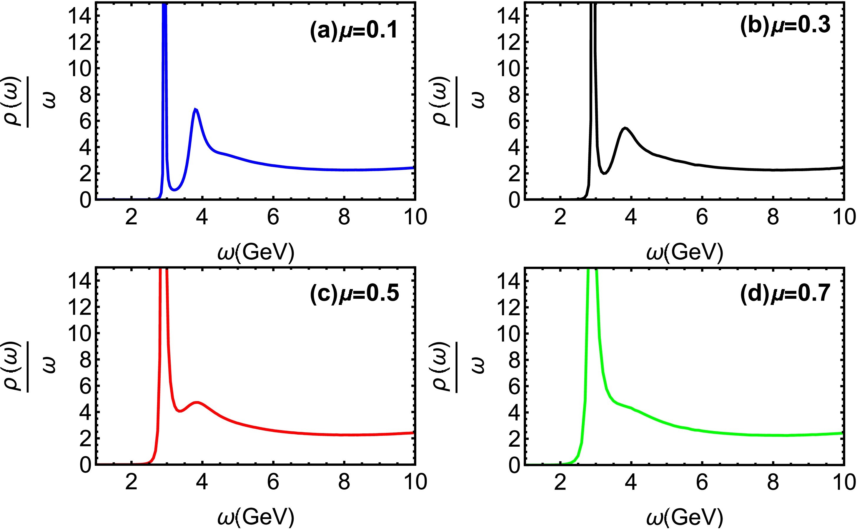
Figure 2. (color online) Spectral functions of charmonium at
$ T=0.15 $ GeV for different μ.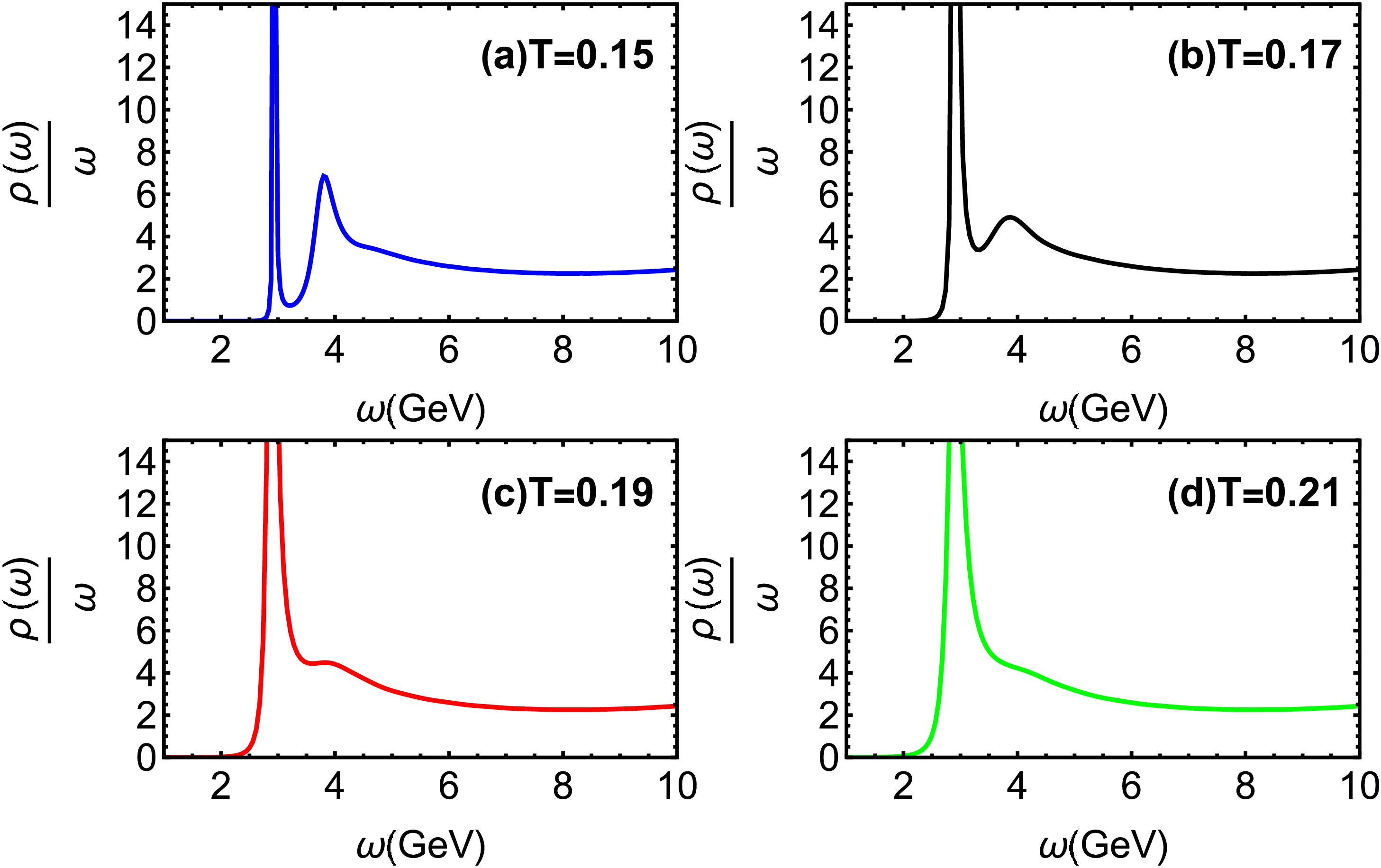
Figure 3. (color online) Spectral functions of charmonium at
$ \mu=0.1 $ GeV for different T.In Fig. 4, charmonium spectral functions are shown at
$ T=0.25 $ GeV for various μ. The$ J/\Psi $ peak exhibits a slight but consistent decrease in height accompanied by noticeable broadening with increasing chemical potentials μ. Figure 5 shows that$ J/\Psi $ dissociates with rising temperature. The ground state progressively dissociates, nearly vanishing at a temperature of$ T = 0.45 $ GeV ($ T=3.52T_c $ ). In Ref. [59], the lattice QCD suggests that the$ J/\Psi $ gradually dissociates and disappears at around$ 3T_c $ . Our finding is in close agreement with lattice QCD simulations [59].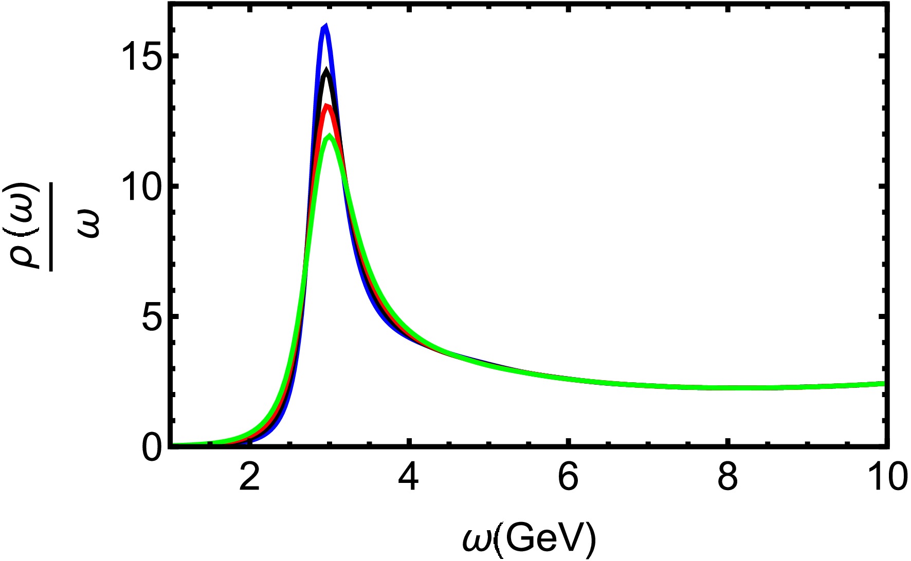
Figure 4. (color online) Spectral functions of charmonium at
$ T=0.25 $ GeV for different μ. The blue, black, red, and green line denote$ \mu = 0.1,\ 0.3,\ 0.5 $ and 0.7 GeV, respectively.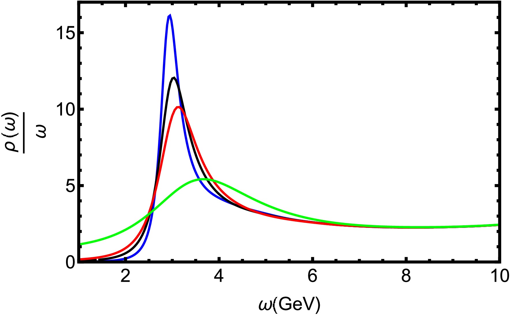
Figure 5. (color online) Spectral functions of charmonium at
$ \mu=0.1 $ GeV for different T. The blue, black, red, and green line denote$ T = 0.25,\ 0.3,\ 0.35 $ and 0.45 GeV, respectively.Figure 6 presents bottomonium spectral functions at
$ T=0.25 $ GeV for different μ. Increasing chemical potential clearly suppresses the 2S state, suggesting that the influence of density on excited quarkonium states. Fig. 7 demonstrates thermal suppression of the 2S state, leading to full dissolution at$ T= 0.31GeV $ ($ T=2.42T_c $ ). Lattice QCD predicts that the lower bound of the$ \Upsilon(1S) $ state dissociates at around$ 2.3T_c $ [60]. Our finding is close to the lattice QCD findings.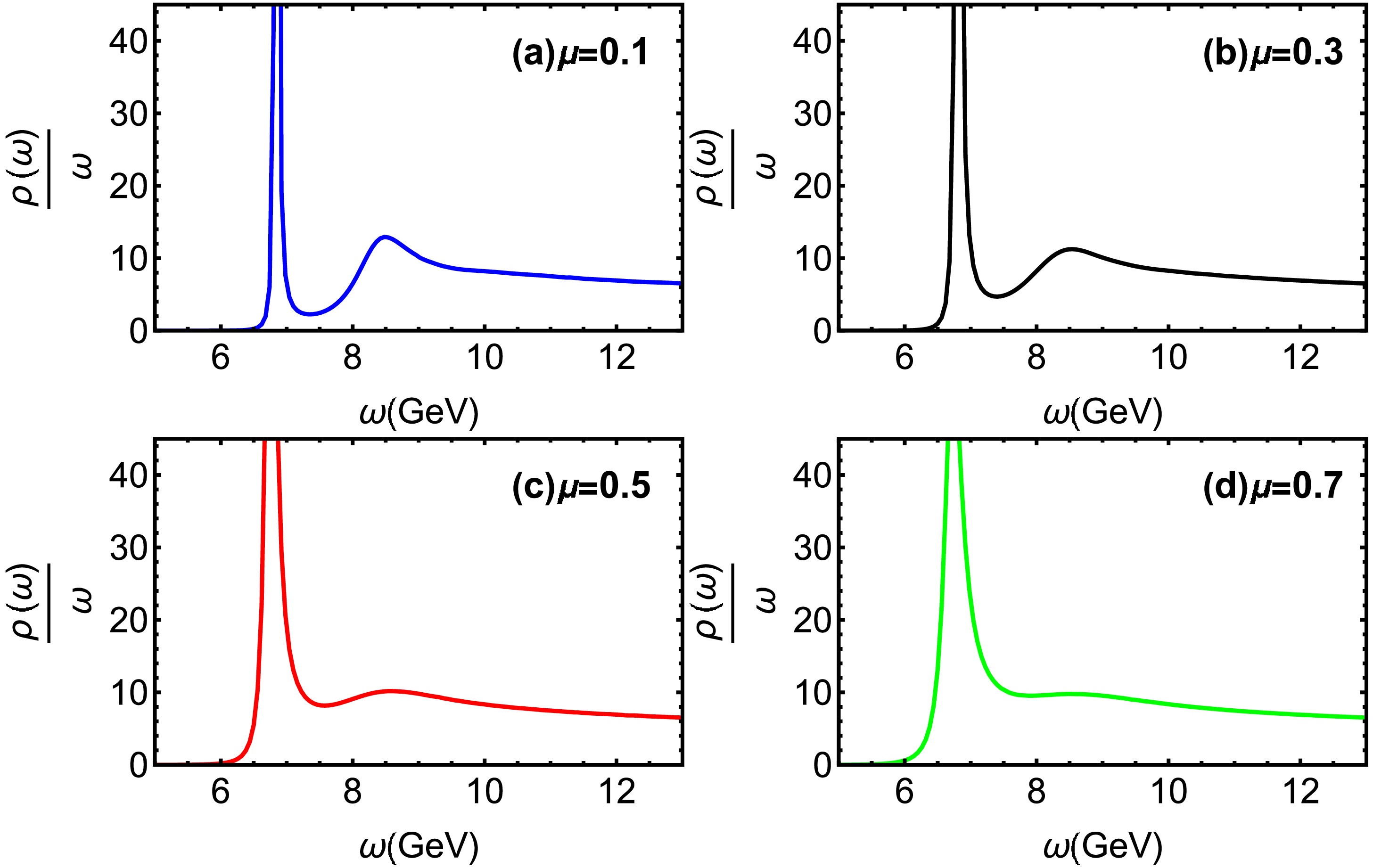
Figure 6. (color online) Spectral functions of bottomonium at
$ T=0.25 $ GeV for different μ.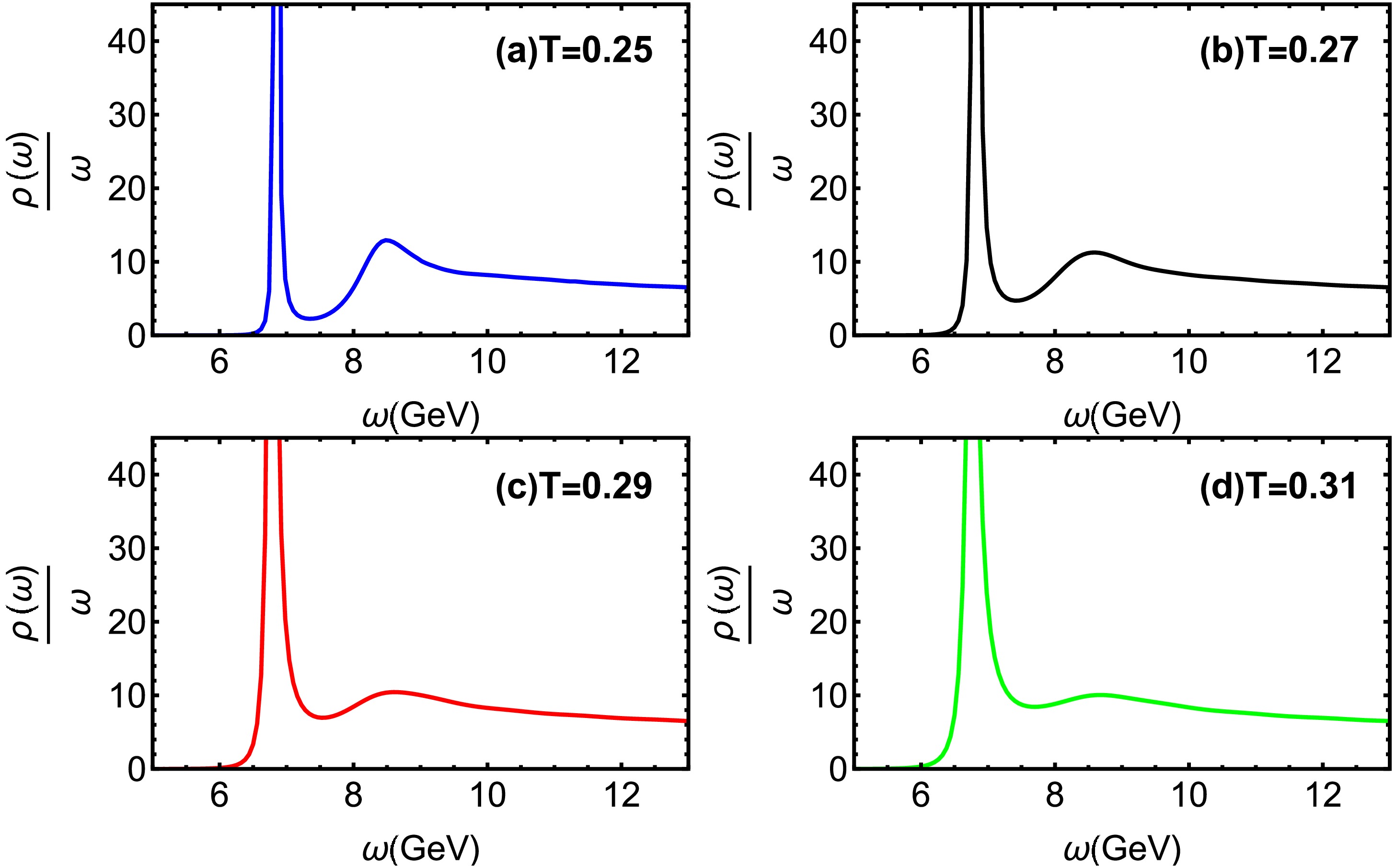
Figure 7. (color online) Spectral functions of bottomonium at
$ \mu=0.1 $ GeV for different T.In Fig. 8, we present the spectral functions of bottomonium at
$ T=0.35 $ GeV for different μ. The bottomonium 1S ($ \Upsilon(1S) $ ) peak exhibits reduced height and increased width with growing μ, indicating strong dissociation in a high density environment. Fig. 9 reveals that the$ \Upsilon(1S) $ state also dissociates at high temperature, melting completely around$ T= 0.55GeV $ ($ T=4.30T_c $ ). From the results, one can find that the excited states dissociate before ground states, and bottomonium states survive to higher temperatures than charmonium due to the larger bottom quark mass and consequently stronger binding.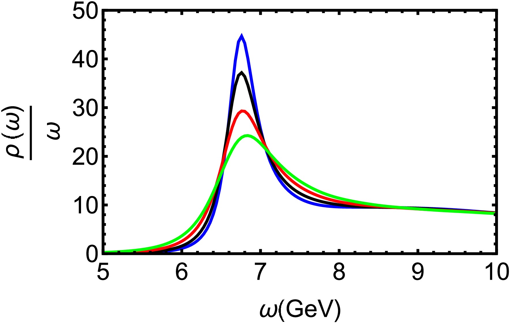
Figure 8. (color online) Spectral functions of bottomonium at
$ T=0.35 $ GeV for different μ. The blue, black, red, and green line denote$ \mu = 0.1,\ 0.3,\ 0.5 $ and 0.7 GeV, respectively.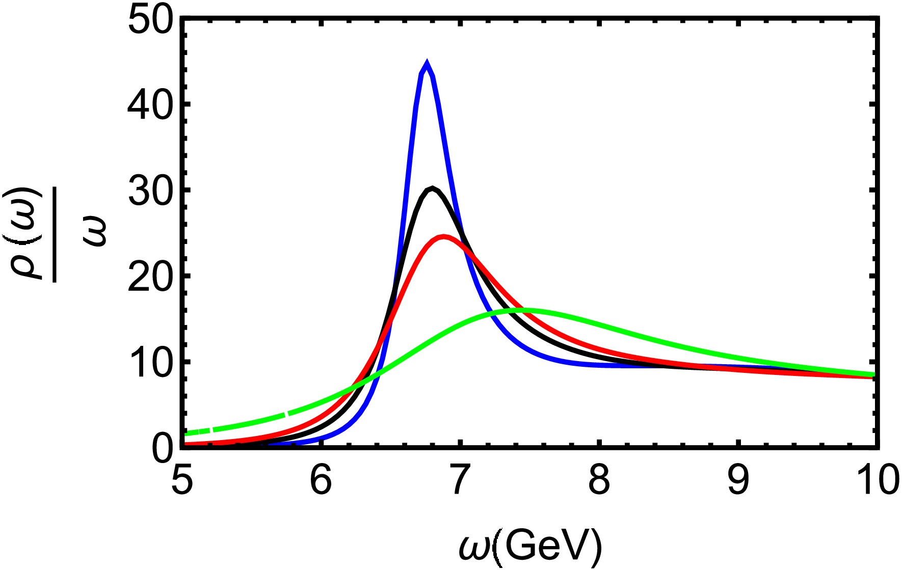
Figure 9. (color online) Spectral functions of bottomonium at
$ \mu=0.1 $ GeV for different T. The blue, black, red, and green line denote$ T = 0.35,\ 0.4,\ 0.45 $ and 0.55 GeV, respectively.In Au+Au collisions at RHIC, STAR measurements demonstrate that the
$ \Upsilon(2S) $ state melts at a lower temperature in the QGP than the$ \Upsilon(1S) $ state [61]. According to lattice QCD calculations [62], charmonia have a lower dissociation temperature than bottomonia, meaning they melt more easily in the QGP due to their weaker binding. Our findings are in close agreement with the STAR results and the lattice QCD simulations of Refs. [61, 62]. The 2S state corresponds to a string configuration extending deeper into the bulk, where it is more susceptible to the influence of the black hole horizon. Its wave function is more spatially extended and thus more easily disrupted by thermal and density perturbations in the medium, leading to its melting at a lower temperature and chemical potential.In [31], the authors discuss the heavy quarkonium dissociation at finite temperature and chemical potential in the soft wall model. Comparing with [31], our model provides a more direct link to QCD thermodynamics via the data-driven background, offering a quantitatively more constrained prediction. A systematic analysis of the peak positions in the spectral functions (Figs. 4, 5, 8, and 9) indicates that the effective mass of heavy quarkonium increases with both temperature and chemical potential, which is consistent with the findings of Ref. [27].
-
Having established the holographic model with its parameters optimized by machine learning, we now proceed to calculate the spectral functions for heavy quarkonium within this optimized framework. The expressions for the spectral function are provided in Ref. [26]. The heavy quarkonium is modeled by the vector field
$ V_m = (V_\mu, V_z) $ , which is holographically dual to the gauge theory current$ J^\mu = \overline{\Psi}\gamma^\mu\Psi $ . The corresponding gravitational action is given by [26]$ \begin{aligned} I= \int {\rm d}^{4}x {\rm d} z \sqrt{-g} \, {\rm e}^{-\phi(z)}\bigg[-\frac{1}{4g^2_5 }F_{mn}F^{mn} \bigg], \end{aligned} $
(13) where
$ F_{mn}=\partial_m V_n -\partial_n V_m $ . For simplicity, the coupling$ g^2_5 $ is set to unity. The dilaton profile$ \phi(z) $ is adopted from Ref. [26]:$ \begin{aligned} \phi(z)= w^2 z^2+Mz+\tanh\left(\frac{1}{Mz}-\frac{w}{\sqrt{\Gamma}}\right), \end{aligned} $
(14) where w and Γ represent the quark mass and string tension, respectively. M denotes a mass scale associated with non-hadronic decay.
We apply the dilaton profile of Eq. (14) to calculate heavy quarkonium spectral functions. Our choice of this combination was motivated by both physical reasoning and practical feasibility. The dilaton profile from Ref. [26] was specifically designed to capture the decay constants of heavy quarkonium, and it has been validated against experimental data. Conversely, the EMD background from Refs. [55, 56] was optimized to accurately reproduce the bulk thermodynamic properties (equation of state) of QCD. Our aim is to study a heavy quarkonium probe within a medium that faithfully represents the QCD thermodynamic. This strategy of using a probe-specific dilaton within a bulk-optimized metric is common and effective, as evidenced in several holographic studies (e.g., Refs. [26, 27, 30, 31, 34−41]).
We agree that the full self-consistent approach would be to use the dilaton field obtained simultaneously with the metric in the machine-learning procedure of Refs. [55, 56]. However, the primary objective of that work was to fit the equation of state; therefore, the resulting dilaton is optimized for bulk thermodynamics and is not necessarily tailored to describe the detailed structure of heavy meson states. The use of a dilaton proven for heavy quarkonium (from Ref. [26]) within a background proven for bulk QCD thermodynamics represents a pragmatic and physically justified compromise to address our specific research question.
These parameters of Eq. (14) for charmonium and bottomonium are given as follows [26]:
$ \begin{aligned}[b] & w_c=1.2 \;{\rm GeV}, \sqrt{\Gamma_c}=0.55\;{\rm GeV}, M_c = 2.2\;{\rm GeV};\\ & w_b=2.45\;{\rm GeV}, \sqrt{\Gamma_b}=1.55\;{\rm GeV}, M_b = 6.2\;{\rm GeV}. \end{aligned} $
(15) Within the framework of the membrane paradigm, the spectral function for heavy mesons can be derived [58]. We first rewrite the background form (Eq. (2))
$ \begin{aligned} {\rm d}s^2= -g_{tt}{\rm d}t^2 +g_{xx_{1}} {\rm d} x_{1}^{2}+ g_{xx_{2}} {\rm d} x_{2}^{2}+g_{xx_{3}} {\rm d} x_{3}^{2}+g_{zz} {\rm d} z^2, \end{aligned} $
(16) where
$g_{tt}=\dfrac{L^2 {\rm e}^{2 A(z)}}{z^2} g(z)$ ,$g_{xx_{1}}=g_{xx_{2}}=g_{xx_{3}}=\dfrac{L^2 {\rm e}^{2 A(z)}}{z^2}$ , and$g_{zz}=\dfrac{L^2 {\rm e}^{2 A(z)}}{g(z) z^2}$ .The equation of motion is obtained from Eq. (13):
$ \begin{aligned} \partial^m \bigg(\frac{\sqrt{-g}}{h(z)}F_{mn}\bigg)=0, \end{aligned} $
(17) where
$h(z)={\rm e}^{\phi(z)}$ .The conjugate momentum of the gauge field for a z-foliation is given by
$ \begin{aligned} j^\mu= -Q F^{z\mu}. \end{aligned} $
(18) The background described by Eq. (18) is isotropic in the
$ \overrightarrow{x} $ -direction. The equations of motion exhibit longitudinal fluctuations in the ($ t, x_3 $ ) plane and transverse fluctuations in the ($ x_1, x_2 $ ) plane. The longitudinal components of Eq. (17) are given by$ \begin{aligned}[b] & -\partial_z j^t -\frac{\sqrt{-g}}{h(z)}g^{tt}g^{xx_3}\partial_{x_3}F_{x_3 t}=0,\\ & -\partial_z j^{x_3} +\frac{\sqrt{-g}}{h(z)}g^{tt}g^{xx_3}\partial_{t}F_{x_3 t}=0.\\ & \partial_{x_3} j^{x_3}+\partial_t j^t =0. \end{aligned} $
(19) Applying the Bianchi identity yields
$ \begin{aligned} \partial_z F_{x_3 t}-\frac{h(z)}{\sqrt{-g}}g_{zz}g_{xx_3}\partial_t j^z -\frac{h(z)}{\sqrt{-g}} g_{tt}g_{xx_3}\partial_{x_3}j^t=0. \end{aligned} $
(20) The conductivity and its derivative for the longitudinal channel are
$ \begin{aligned}[b]& \overline{\sigma}_L (\omega,\overrightarrow{p},z)=\frac{j^{x_3}(\omega,\overrightarrow{p},z)}{F_{x_3 t}(\omega,\overrightarrow{p},z)},\\ & \partial_z \overline{\sigma}_L=-{\rm i}\omega\sqrt{\frac{g_{zz}}{g_{tt}}}\bigg[\Sigma(z)-\frac{\overline{\sigma}^2_L}{\Sigma(z)}\Bigg(1-\frac{p^2_3}{\omega^2}\frac{g^{xx_3}}{g^{tt}}\Bigg) \bigg], \end{aligned} $
(21) where the momentum
$ p=(\omega,0,0,p_3) $ and$ \Sigma(z)= \dfrac{1}{h(z)}\sqrt{\dfrac{-g}{g_{zz}g_{tt}}}g^{xx_3} $ .Similarly, the results for the transverse channel are obtained
$ \begin{aligned} \partial_z \overline{\sigma}_T={\rm i}\omega \sqrt{\frac{g_{zz}}{g_{tt}}} \bigg[\frac{\overline{\sigma}^2_T}{\Sigma(z)}- \Sigma(z)\Bigg(1-\frac{p^2_3}{\omega^2}\frac{g^{xx_3}}{g^{tt}}\Bigg) \bigg]. \end{aligned} $
(22) For vanishing momentum (
$ p^2_3 =0 $ ), the conductivities satisfy$ \overline{\sigma}= \overline{\sigma}_T = \overline{\sigma}_L $ , with the explicit expression given by$ \begin{aligned} \partial_z \overline{\sigma}={\rm i}\omega \sqrt{\frac{g_{zz}}{g_{tt}}} \bigg[\frac{\overline{\sigma}^2}{\Sigma(z)}- \Sigma(z) \bigg]. \end{aligned} $
(23) According to the Kubo formula, the AC conductivity σ is given by the retarded Green's function
$ \begin{aligned} \sigma(\omega)=-\frac{G_R (\omega)}{{\rm i} \omega}\equiv \overline{\sigma}(\omega,z=0). \end{aligned} $
(24) The spectral function is subsequently derived as
$ \begin{aligned} \rho(\omega)\equiv -{\rm Im} G_R (\omega)=\omega {\rm Re} \overline{\sigma}(\omega,0). \end{aligned} $
(25) Figure 2 displays the spectral functions of charmonium at
$ T=0.15 $ GeV for different chemical potentials μ. The quasiparticle states are identified by the bell-shaped spectral profiles, with the first and second peaks corresponding to the 1S ($ J/\Psi $ ) and 2S states, respectively. As the baryon chemical potential increases, the 2S state undergoes significant suppression, indicating its heightened sensitivity to the dense baryonic environment. Figure 3 illustrates spectral functions at$ \mu=0.1 $ GeV for different temperatures. We observe that the 2S state experiences considerable broadening and a reduction in peak height, indicating that the 2S state progressively weakens with increasing T. The 2S state undergoes complete dissolution at a critical temperature of$ T = 0.21 $ GeV ($ T= 1.64T_c $ ).
Figure 2. (color online) Spectral functions of charmonium at
$ T=0.15 $ GeV for different μ.
Figure 3. (color online) Spectral functions of charmonium at
$ \mu=0.1 $ GeV for different T.In Fig. 4, charmonium spectral functions are shown at
$ T=0.25 $ GeV for various μ. The$ J/\Psi $ peak exhibits a slight but consistent decrease in height accompanied by noticeable broadening with increasing μ. Figure 5 shows that$ J/\Psi $ dissociates with increasing temperature. The ground state progressively dissociates, nearly vanishing at a temperature of$ T = 0.45 $ GeV ($ T=3.52T_c $ ). In Ref. [59], the lattice QCD suggests that$ J/\Psi $ gradually dissociates and disappears at around$ 3T_c $ . Our finding is in close agreement with lattice QCD simulations [59].
Figure 4. (color online) Spectral functions of charmonium at
$ T=0.25 $ GeV for different μ. The blue, black, red, and green lines denote$ \mu = 0.1,\ 0.3,\ 0.5 $ , and 0.7 GeV, respectively.
Figure 5. (color online) Spectral functions of charmonium at
$ \mu=0.1 $ GeV for different T. The blue, black, red, and green line denote$ T = 0.25,\ 0.3,\ 0.35 $ and 0.45 GeV, respectively.Figure 6 presents bottomonium spectral functions at
$ T=0.25 $ GeV for different μ. Increasing the chemical potential clearly suppresses the 2S state, suggesting the influence of density on excited quarkonium states. Figure 7 demonstrates thermal suppression of the 2S state, leading to full dissolution at$T= 0.31\; {\rm GeV}$ ($ T=2.42T_c $ ). Lattice QCD predicts that the lower bound of the$ \Upsilon(1S) $ state dissociates at around$ 2.3T_c $ [60]. Our finding is close to the lattice QCD findings.
Figure 6. (color online) Spectral functions of bottomonium at
$ T=0.25 $ GeV for different μ.
Figure 7. (color online) Spectral functions of bottomonium at
$ \mu=0.1 $ GeV for different T.In Fig. 8, we present the spectral functions of bottomonium at
$ T=0.35 $ GeV for different μ. The bottomonium 1S ($ \Upsilon(1S) $ ) peak exhibits reduced height and increased width with increasing μ, indicating strong dissociation in a high density environment. Figure 9 reveals that the$ \Upsilon(1S) $ state also dissociates at high temperatures, melting completely around$ T= 0.55\; {\rm GeV} $ ($ T=4.30T_c $ ). These indicate that the excited states dissociate before ground states, and bottomonium states survive to higher temperatures than charmonium owing to the larger bottom quark mass and consequently stronger binding.
Figure 8. (color online) Spectral functions of bottomonium at
$ T=0.35 $ GeV for different μ. The blue, black, red, and green lines denote$ \mu = 0.1,\ 0.3,\ 0.5 $ , and 0.7 GeV, respectively.
Figure 9. (color online) Spectral functions of bottomonium at
$ \mu=0.1 $ GeV for different T. The blue, black, red, and green lines denote$ T = 0.35,\ 0.4,\ 0.45 $ , and 0.55 GeV, respectively.In Au+Au collisions at RHIC, STAR measurements demonstrate that the
$ \Upsilon(2S) $ state melts at a lower temperature in the QGP than the$ \Upsilon(1S) $ state [61]. According to lattice QCD calculations [62], charmonia have a lower dissociation temperature than bottomonia, meaning they melt more easily in the QGP owing to their weaker binding. Our findings are in close agreement with the STAR results and the lattice QCD simulations of Refs. [61, 62]. The 2S state corresponds to a string configuration extending deeper into the bulk, where it is more susceptible to the influence of the black hole horizon. Its wave function is more spatially extended and thus more easily disrupted by thermal and density perturbations in the medium, leading to its melting at a lower temperature and chemical potential.In [31], the authors discuss the heavy quarkonium dissociation at finite temperature and chemical potential in the soft wall model. Compared with [31], our model provides a more direct link to QCD thermodynamics via the data-driven background, offering a quantitatively more constrained prediction. A systematic analysis of the peak positions in the spectral functions (Figs. 4, 5, 8, and 9) indicates that the effective mass of heavy quarkonium increases with both temperature and chemical potential, which is consistent with the findings of Ref. [27].
-
In this work, we investigate the dissociation of heavy quarkonium in the framework of a data-driven holographic QCD model. The parameters of the EMD model were calibrated based on lattice QCD data via a machine-learning approach.
We systematically examine the influence of baryon chemical potential μ and temperature T on the spectral functions of both charmonium and bottomonium. Our results demonstrate that increasing either the baryon chemical potential or temperature suppresses the quasiparticle peaks associated with the 1S and 2S states, thereby promoting the dissociation of heavy quarkonia. An increase in temperature or chemical potential moves the black hole horizon in the bulk geometry closer to the boundary. This decreases the binding energy between the quark and antiquark, making it harder to maintain a bound state [57]. Consequently, the quasiparticle peaks in the spectral function broaden and their heights are suppressed. Specifically, the 2S state is found to be more susceptible to melting under external conditions compared with the ground states. These findings agree with lattice QCD simulations. This study underscores the utility of data-driven gravitational modeling for exploring nonperturbative QCD phenomena under extreme conditions.
This work is a systematic study of heavy quarkonium dissociation at finite temperature and finite baryon chemical potential within a data-driven holographic model. This enables us to explore regions of finite density that are challenging for lattice QCD. We also highlight the predictive power of our model for the dissociation patterns of both charmonium and bottomonium states. The interplay between the model framework and specific dilaton field used in this study is important to investigate. A limitation of the present study is the use of the dilaton profile from [26] instead of the machine-learned dilaton from the EMD framework [55, 56]. A direct comparison using the fully self-consistent machine-learned dilaton will be an important future task for predicting quarkonium dissociation. Comparing those future results with the ones presented here would provide a direct test of how the data-driven parameter optimization for quarkonium dissociation.
-
In this work, we investigate the dissociation of heavy quarkonium in the framework of a data-driven holographic QCD model.The parameters of the EMD model were calibrated based on lattice QCD data via a machine learning approach.
We systematically examined the influence of baryon chemical potential μ and temperature T on the spectral functions of both charmonium and bottomonium. Our results demonstrate that increasing either the baryon chemical potential or temperature suppresses the quasiparticle peaks associated with the 1S and 2S states, thereby promoting the dissociation of heavy quarkonia. An increase in temperature or chemical potential moves the black hole horizon in the bulk geometry closer to the boundary. This decreases the binding energy between the quark and antiquark, making it harder to maintain a bound state [57]. Consequently, the quasiparticle peaks in the spectral function broaden and their heights are suppressed. Specifically, the 2S state is found to be more susceptible to melting under external conditions compared to the ground states. These findings agree with lattice QCD simulations. This study underscores the utility of data-driven gravitational modeling for exploring nonperturbative QCD phenomena under extreme conditions.
This work is the systematic study of heavy quarkonium dissociation at finite temperature and finite baryon chemical potential within a data-driven holographic model. This allows us to explore regions of finite density that are challenging for lattice QCD. We also highlight the predictive power of our model for the dissociation patterns of both charmonium and bottomonium states. It is important to discuss the interplay between the model framework and the specific dilaton field used in this study. A limitation of the present study is the use of the dilaton profile from [26] instead of the machine-learned dilaton from the EMD framework [55, 56]. A direct comparison using the fully self-consistent machine-learned dilaton will be an important future task for predicting quarkonium dissociation. Comparing those future results with the ones presented here would provide a direct test of how the data-driven parameter optimization for quarkonium dissociation.
Dissociation of heavy quarkonium from a data-driven holographic QCD model
- Received Date: 2025-10-22
- Available Online: 2026-04-15
Abstract: In this work, we study the dissociation of heavy quarkonium from a data-driven holographic QCD model. The model parameters were optimized using machine learning, which successfully reproduced lattice QCD data. Subsequently, we explore the spectral function for charmonium and bottomonium at finite temperature and baryon chemical potential, focusing on the behavior of the 1S and 2S states. Our results show that increasing the temperature or chemical potential strongly suppresses the quasiparticle peaks, with the 2S state dissolving earlier than the 1S ground state. The charmonium 2S state melts completely around $ 1.64T_c $ ($ T_c $ is the critical temperature), whereas the bottomonium 2S state disappears near $ 2.42T_c $. $ J/\Psi $ nearly vanishes at $ 3.52T_c $, and the $ \Upsilon(1S) $ state melts completely around $ 4.30T_c $. The results correspond with lattice QCD predictions and demonstrate the effectiveness of data-driven holographic models in understanding hard probes in the quark-gluon plasma.


 DownLoad: