


 Abstract
 HTML
HTML Reference
 Related
 PDF
PDF


-
Searches for additional scalar Higgs boson productions in many extensions of the Standard Model (SM) are a key motivation for the construction of future colliders, including the High-Luminosity LHC (HL-LHC) and proposed lepton colliders such as the International Linear Collider (ILC) and muon–TeV colliders. The discovery of the additional scalar Higgs bosons would provide direct evidence for new physics and would also offer enhanced insight into the dynamics of electroweak symmetry breaking (EWSB). In all possible production channels of exotic scalar states, singly charged Higgs boson productions have recently received particular attention at colliders. Experimentally, searches for charged Higgs bosons in the light mass regions produced in top-quark decay have been detected at
$ \sqrt{s}=7 $ and$ 8 $ TeV at the LHC [1−4]. The ATLAS collaboration has pursued additional explorations of charged Higgs bosons following decay channels$ H^{+} \to \tau\nu $ [5] and$ H^+ \to c\bar{s} $ [6]. For heavier charged Higgs states, both ATLAS and CMS have conducted searches through decay channels such as$ H^{\pm} \to tb $ [7−9],$ H^{\pm} \to W^{\pm}Z $ [10, 11] at$ \sqrt{s}=8 $ TeV, and via vector boson fusion production at$ \sqrt{s}=13 $ TeV [12]. Furthermore, searches for$ H^\pm \to cb/cs $ at$ \sqrt{s}=8 $ TeV have been reported in Refs. [13, 14], while the$ H^{\pm}\to HW^{\pm} $ decay mode has been studied at$ \sqrt{s}=13 $ TeV [15, 16]. More recently, both ATLAS and CMS investigated charged Higgs bosons in association with top quarks and in top-quark decay, wherein both production channels were analyzed with the subsequent decay$ H^{\pm}\to \tau^{\pm} \nu_{\tau} $ [17−19].Theoretically, charged Higgs boson production at the LHC has been calculated within many BSM scenarios. In THDM,
$ pp \to tH^- \to tW^-b\bar{b} $ production has been computed, including top-quark polarization effects as discussed in Ref. [20, 21]. Additionally, the decay$ H^+ \to t\bar{b} $ has been systematically examined in the Minimal Supersymmetric SM (MSSM) [22]. The production of charged Higgs boson pairs at the HL-LHC has been investigated in Ref. [23]. Charged Higgs bosons in the light-mass regions decaying into electroweak vector bosons have been analyzed based on Run III data [24]. Investigations of the productions for$ pp \to H^{\pm}h/A $ and$ pp \to H^{+}H^{-} $ with$ H^{\pm}\to W^{\pm}h/A $ have been carried out in Ref. [25]. Further studies on charged Higgs bosons at the LHC have been reported in Refs. [26−28], including analyses of production via vectorlike top-quark pairs [29−34] and studies on the$ W\gamma $ decay mode [35]. Production of charged Higgs bosons at future lepton colliders has been studied at$ \mu^+\mu^- $ and$ e^+e^- $ machines [36−39]. Moreover, heavy charged Higgs states at$ \gamma\gamma $ colliders have been probed using multivariate analyses including the$ H^{\pm}\to W^{\pm}H $ decay channel [40, 41]. Ref. [42] has shown that new physics effects from scalar Higgs exchange in the loop can be probed through electroweak corrections to the process$ e^- e^+ \to h \nu_e \nu_e $ at$ e^+e^- $ machines.In comparison with hadron colliders, muon–TeV colliders provide a clean leptonic collision environment for high-precision tests, similar to
$ e^- e^+ $ collisions. Moreover, they also open the door to a high-energy frontier from which to probe physics beyond the SM [43, 44]. Given that the mass of the muon is greater than that of the the electron by a factor of roughly 207, the contributions of neutral-Higgs exchange in the s-channel may be enhanced due to resonance effects. Last but not least, the coupling of charged scalar Higgs bosons to muons is proportional to$ \tan\beta $ or$ \cot\beta $ depending on the type of THDM. As a result, these effects could provide an opportunity to distinguish among the four types of THDM. Second, loop–induced decay$ H^{\pm} \to W^{\pm}Z $ is sensitive to BSM effects and provides important information for discriminating among different types of THDM. This decay process was computed in Ref. [45]. Alternative calculations including the CP-violating THDM have been presented in Refs. [46−50]. In this work, one-loop contributions for decay$ H^{\pm} \to W^{\pm}Z $ in THDM are computed and their implications for future muon–TeV colliders are studied. In contrast to other works, our calculations are performed in the general$ {\cal{R}}_{\xi} $ gauge and the results are verified through several self-consistency checks such as the ξ-independence, renormalization-scale stability, and ultraviolet (UV) finiteness of the amplitude. Many previous studies have shown [51] that charged Higgs masses vary widely from$ {\cal{O}}(100) $ GeV to approximately1000 GeV in Type-I and Type-X of THDM, whereas they are typically greater than$ 500 $ GeV in the other types of THDM. Thus, the Type-I and Type-X models are of particular interest in searching for charged Higgs bosons in the low-mass regions, especially around the$ m_W + m_Z $ threshold. We emphasize that the phenomenological results for the Type-I case were presented in our previous work [52]. In this paper, we present a phenomenological analysis of the Type-X THDM based on an updated viable parameter space. Charged Higgs pair production is then studied via$ \mu^+\mu^- \to H^+H^- \to W^{\pm}W^{\mp}Zh $ and$ \mu^+\mu^- \to \gamma\gamma \to H^+H^- \to W^{\pm}W^{\mp}Zh $ , with signals evaluated with respect to the SM backgrounds.The remainder of this paper is structured as follows. In Section II, we review the THDM framework, its constraints, and the updated parameter-space scan for the Type-X THDM. In Section III, we present the one-loop calculation of
$ H^{\pm} \to W^{\pm}Z $ along with numerical checks of the computation. We then discuss the phenomenological applications in Section IV. Section V concludes by summarizing our findings. Analytic expressions and checks of ξ-independence are provided in the appendices. -
Searches for additional scalar Higgs boson productions in many extensions of the Standard Model (SM) are one of the main purposes of future colliders, including the High-Luminosity LHC (HL-LHC) and proposed lepton colliders such as the International Linear Collider (ILC) and muon–TeV colliders. The discovery of the additional scalar Higgs bosons would provide direct evidence for new physics and would also offer a enhanced insight into the dynamics of electroweak symmetry breaking (EWSB). In all possible production channels of exotic scalar states, singly charged Higgs boson productions have recently received particular attention at colliders. Experimentally, searches for charged Higgs bosons in the light mass regions, produced in top-quark decays have been detected at
$ \sqrt{s}=7 $ and$ 8 $ TeV at the LHC as in Refs. [1−4]. Additional exploration of charged Higgs bosons following decay channels$ H^{+} \to \tau\nu $ [5] and$ H^+ \to c\bar{s} $ [6], have also been examined by the ATLAS Collaboration. For heavier charged Higgs states, both ATLAS and CMS have conducted searches through decay channels such as$ H^{\pm} \to tb $ [7−9],$ H^{\pm} \to W^{\pm}Z $ [10, 11] at$ \sqrt{s}=8 $ TeV, and via vector boson fusion production at$ \sqrt{s}=13 $ TeV [12]. Furthermore, searches for$ H^\pm \to cb/cs $ at$ \sqrt{s}=8 $ TeV have been reported in Refs. [13, 14], while the$ H^{\pm}\to HW^{\pm} $ decay mode has been studied at$ \sqrt{s}=13 $ TeV [15, 16]. More recently, both ATLAS and CMS have carried out the investigations for charged Higgs bosons in association with top quarks and in top-quark decays, in which both production channels have been analyzed with the subsequent decay$ H^{\pm}\to \tau^{\pm} \nu_{\tau} $ [17−19].Theoretically, charged Higgs boson production at the LHC has been calculated within many BSM scenarios. In the THDM,
$ pp \to tH^- \to tW^-b\bar{b} $ production has been computed, including top-quark polarization effects as discussed in [20, 21]. Additionally, the decay$ H^+ \to t\bar{b} $ has been systematically examined in the Minimal Supersymmetric Standard Model (MSSM) [22]. The production of charged Higgs boson pairs at the HL-LHC has been investigated in [23]. Taking Run III data, charged Higgs bosons in the light-mass regions decaying into electroweak vector bosons have been analyzed in the report [24]. Investigations of the productions for$ pp \to H^{\pm}h/A $ and$ pp \to H^{+}H^{-} $ with$ H^{\pm}\to W^{\pm}h/A $ have also been carried out in Ref. [25]. Further studies on charged Higgs bosons at the LHC have also presented in Refs. [26−28], including analyses of production via vectorlike top-quark pairs [29−34] and studies of the$ W\gamma $ decay mode [35]. Production of charged Higgs bosons at future lepton colliders has also been studied at$ \mu^+\mu^- $ and$ e^+e^- $ machines [36−39]. Furthermore, heavy charged Higgs states at$ \gamma\gamma $ colliders have been probed using multivariate analyses including the$ H^{\pm}\to W^{\pm}H $ decay channel [40, 41]. In Ref. [42], new physics effects from scalar Higgs exchange in the loop can be probed through electroweak corrections to the process$ e^- e^+ \to h \nu_e \nu_e $ at$ e^+e^- $ machines.In comparison with hadron colliders, a muon–TeV collider provides a clean leptonic collision environment for high-precision tests, similar to
$ e^- e^+ $ collisions. Moreover, muon–TeV colliders offer a high-energy frontier for probing physics beyond the Standard Model, as studied in Refs. [43, 44]. Since the muon mass is about 207 times larger than the electron mass, the contributions from neutral-Higgs exchange in the s-channel may be enhanced due to resonance effects. Last but not least, the coupling of charged scalar Higgs bosons to muons is proportional to$ \tan\beta $ or$ \cot\beta $ , depending on the type of THDM. As a result, these effects could provide an opportunity to distinguish among the four types of THDM. Secondly, loop–induced decay$ H^{\pm} \to W^{\pm}Z $ is sensitive to BSM effects and provides important information for discriminating among different types of THDM. This decay process was computed in Ref. [45]. Alternative calculations with including the CP-violating THDM, have been presented in [46−50]. In this work, one-loop contributions for decay$ H^{\pm} \to W^{\pm}Z $ in the THDM are computed and its implications at future muon–TeV colliders are studied. Different from other works, our calculations are performed in the general$ {\cal{R}}_{\xi} $ gauge, and results are verified through several self-consistency checks such as the ξ-independence, renormalization-scale stability and ultraviolet (UV) finiteness of the amplitude. From many previous references, for example Ref. [51], charged Higgs masses vary widely from$ {\cal{O}}(100) $ GeV to about 1000 GeV in the Type-I and Type-X of THDM, while they are typically greater than$ 500 $ GeV in other types of THDM. For this reason, the Type-I and Type-X models are of particular interest for searching for charged Higgs bosons in the low-mass regions, especially around the$ m_W + m_Z $ threshold. It is emphasized that the phenomenological results for the Type-I case were presented in our previous work [54]. In this paper, we present the phenomenological analysis of the Type-X THDM based on the updated viable parameter space. Charged Higgs pair production is then studied via$ \mu^+\mu^- \to H^+H^- \to W^{\pm}W^{\mp}Zh $ and$ \mu^+\mu^- \to \gamma\gamma \to H^+H^- \to W^{\pm}W^{\mp}Zh $ , with signals evaluated with respect to the SM backgrounds.Our paper has the following structure. Reviewing of the THDM framework, its constraints, and the updated parameter-space scan for the Type-X THDM are presented in Section 2. Section 3 presents the one-loop calculation of
$ H^{\pm} \to W^{\pm}Z $ along with numerical checks of the computation. Section 4 discusses the phenomenological applications of this work. Section 5 is devoted to the conclusions. Analytic expressions and checks of ξ-independence are provided in the appendices. -
Searches for additional scalar Higgs boson productions in many extensions of the Standard Model (SM) are a key motivation for the construction of future colliders, including the High-Luminosity LHC (HL-LHC) and proposed lepton colliders such as the International Linear Collider (ILC) and muon–TeV colliders. The discovery of the additional scalar Higgs bosons would provide direct evidence for new physics and would also offer enhanced insight into the dynamics of electroweak symmetry breaking (EWSB). In all possible production channels of exotic scalar states, singly charged Higgs boson productions have recently received particular attention at colliders. Experimentally, searches for charged Higgs bosons in the light mass regions produced in top-quark decay have been detected at
$ \sqrt{s}=7 $ and$ 8 $ TeV at the LHC [1−4]. The ATLAS collaboration has pursued additional explorations of charged Higgs bosons following decay channels$ H^{+} \to \tau\nu $ [5] and$ H^+ \to c\bar{s} $ [6]. For heavier charged Higgs states, both ATLAS and CMS have conducted searches through decay channels such as$ H^{\pm} \to tb $ [7−9],$ H^{\pm} \to W^{\pm}Z $ [10, 11] at$ \sqrt{s}=8 $ TeV, and via vector boson fusion production at$ \sqrt{s}=13 $ TeV [12]. Furthermore, searches for$ H^\pm \to cb/cs $ at$ \sqrt{s}=8 $ TeV have been reported in Refs. [13, 14], while the$ H^{\pm}\to HW^{\pm} $ decay mode has been studied at$ \sqrt{s}=13 $ TeV [15, 16]. More recently, both ATLAS and CMS investigated charged Higgs bosons in association with top quarks and in top-quark decay, wherein both production channels were analyzed with the subsequent decay$ H^{\pm}\to \tau^{\pm} \nu_{\tau} $ [17−19].Theoretically, charged Higgs boson production at the LHC has been calculated within many BSM scenarios. In THDM,
$ pp \to tH^- \to tW^-b\bar{b} $ production has been computed, including top-quark polarization effects as discussed in Ref. [20, 21]. Additionally, the decay$ H^+ \to t\bar{b} $ has been systematically examined in the Minimal Supersymmetric SM (MSSM) [22]. The production of charged Higgs boson pairs at the HL-LHC has been investigated in Ref. [23]. Charged Higgs bosons in the light-mass regions decaying into electroweak vector bosons have been analyzed based on Run III data [24]. Investigations of the productions for$ pp \to H^{\pm}h/A $ and$ pp \to H^{+}H^{-} $ with$ H^{\pm}\to W^{\pm}h/A $ have been carried out in Ref. [25]. Further studies on charged Higgs bosons at the LHC have been reported in Refs. [26−28], including analyses of production via vectorlike top-quark pairs [29−34] and studies on the$ W\gamma $ decay mode [35]. Production of charged Higgs bosons at future lepton colliders has been studied at$ \mu^+\mu^- $ and$ e^+e^- $ machines [36−39]. Moreover, heavy charged Higgs states at$ \gamma\gamma $ colliders have been probed using multivariate analyses including the$ H^{\pm}\to W^{\pm}H $ decay channel [40, 41]. Ref. [42] has shown that new physics effects from scalar Higgs exchange in the loop can be probed through electroweak corrections to the process$ e^- e^+ \to h \nu_e \nu_e $ at$ e^+e^- $ machines.In comparison with hadron colliders, muon–TeV colliders provide a clean leptonic collision environment for high-precision tests, similar to
$ e^- e^+ $ collisions. Moreover, they also open the door to a high-energy frontier from which to probe physics beyond the SM [43, 44]. Given that the mass of the muon is greater than that of the the electron by a factor of roughly 207, the contributions of neutral-Higgs exchange in the s-channel may be enhanced due to resonance effects. Last but not least, the coupling of charged scalar Higgs bosons to muons is proportional to$ \tan\beta $ or$ \cot\beta $ depending on the type of THDM. As a result, these effects could provide an opportunity to distinguish among the four types of THDM. Second, loop–induced decay$ H^{\pm} \to W^{\pm}Z $ is sensitive to BSM effects and provides important information for discriminating among different types of THDM. This decay process was computed in Ref. [45]. Alternative calculations including the CP-violating THDM have been presented in Refs. [46−50]. In this work, one-loop contributions for decay$ H^{\pm} \to W^{\pm}Z $ in THDM are computed and their implications for future muon–TeV colliders are studied. In contrast to other works, our calculations are performed in the general$ {\cal{R}}_{\xi} $ gauge and the results are verified through several self-consistency checks such as the ξ-independence, renormalization-scale stability, and ultraviolet (UV) finiteness of the amplitude. Many previous studies have shown [51] that charged Higgs masses vary widely from$ {\cal{O}}(100) $ GeV to approximately1000 GeV in Type-I and Type-X of THDM, whereas they are typically greater than$ 500 $ GeV in the other types of THDM. Thus, the Type-I and Type-X models are of particular interest in searching for charged Higgs bosons in the low-mass regions, especially around the$ m_W + m_Z $ threshold. We emphasize that the phenomenological results for the Type-I case were presented in our previous work [52]. In this paper, we present a phenomenological analysis of the Type-X THDM based on an updated viable parameter space. Charged Higgs pair production is then studied via$ \mu^+\mu^- \to H^+H^- \to W^{\pm}W^{\mp}Zh $ and$ \mu^+\mu^- \to \gamma\gamma \to H^+H^- \to W^{\pm}W^{\mp}Zh $ , with signals evaluated with respect to the SM backgrounds.The remainder of this paper is structured as follows. In Section II, we review the THDM framework, its constraints, and the updated parameter-space scan for the Type-X THDM. In Section III, we present the one-loop calculation of
$ H^{\pm} \to W^{\pm}Z $ along with numerical checks of the computation. We then discuss the phenomenological applications in Section IV. Section V concludes by summarizing our findings. Analytic expressions and checks of ξ-independence are provided in the appendices. -
A detailed review of THDM can be found in Ref. [53]. It is shown that tree-level flavor-changing neutral currents can be prevented by applying a discrete
$ Z_{2} $ symmetry in the Lagrangian, as discussed in Ref. [53]. The different charge quantum numbers of the$ Z_{2} $ for scalar doublets and fermion fields lead to four distinct Yukawa types (known as Type-I, II, X, Y) (see also Ref. [54] for more detail). The Yukawa Lagrangian can be parameterized as$ \begin{aligned}[b] {{\cal{L}}}_\text{Y} =\;& -\sum\limits_{f=u,d,\ell} \left( \sum\limits_{\phi_j=h, H} g_{\phi_j ff}\cdot \phi_j{\overline f}f + g_{Aff}\cdot A {\overline f} \gamma_5f \right) \\ & - \left[ \bar{u}_{i} \left( g_{H^+ u_i d_j}^L m_{u_i} P_L + g_{H^+ u_i d_j}^R m_{d_j} P_R \right)d_{j} H^+ \right] \\& + \cdots \end{aligned} $
(1) $ \begin{aligned}[b]\quad =\;& -\sum\limits_{f=u,d,\ell} \left( \sum\limits_{\phi_j=h, H} \frac{m_f}{v}\xi_{\phi_j}^f \phi_j {\overline f}f -{\rm i} \frac{m_f}{v}\xi_A^f {\overline f} \gamma_5fA \right)\\ & - \frac{ \sqrt{2} }{v} \left[ \bar{u}_{i} V_{ij}\left( m_{u_i} \xi^{u}_A P_L + \xi^{d}_A m_{d_j} P_R \right)d_{j} H^+ \right] \\ & - \frac{\sqrt{2}}{v} \bar{\nu}_L \xi^{\ell}_A m_\ell \ell_R H^+ + \rm{H.c}. \end{aligned} $
(2) In the Lagrangian, the CKM matrix elements are denoted by
$ V_{ij} $ ,$ \ell_{L/R} (\nu_{L/R}) $ represents the left- and right-handed lepton fields, and$ P_{L/R} = (1 \mp \gamma_{5})/2 $ denotes the projection operators. It is easy to check whether the vertices of the charged Higgs with up- and down-type quarks depend linearly on$ \cot\beta $ in the Type-X THDM. As a result, fermionic loop contributions are thus diminished in the large-$ t_{\beta} $ regime.We now turn to the theoretical and experimental bounds on THDM. Theoretical bounds are obtained by imposing conditions such as perturbative unitarity, perturbativity, and vacuum stability, all of which are taken into account in the models under consideration. In the experimental limits, the measured data of the SM-like Higgs properties, the data of flavor observables, and electroweak precision tests are taken into consideration in the constraints. We refer to our previous work [52] for further details about these conditions, wherein the Type-I THDM was studied in greater detail. The parameter space is scanned as follows. We choose parameters for the Type-X THDM within the ranges of
$ s_{\beta-\alpha} \in [0.97,1] $ ,$ t_{\beta} \in [0.5,45] $ ,$ m_{H} \in [130,1000]\; \text{GeV} $ ,$ m_{A,H^{\pm}} \in [130,1000] \; \text{GeV} $ , and$ m_{12}^2 \in [0,10^6]\; \text{GeV}^2 $ , with the SM-like Higgs mass fixed at$ m_{h} = 125.09\; \text{GeV} $ . The sampling points are first tested against theoretical constraints. The allowed points are then checked with the Electroweak Precision Observables (EWPOs). The surviving parameter space is subsequently passed to$ {\mathrm{HiggsBounds-5.10.1}}$ [55] and$ {\mathrm{HiggsSignals-2.6.1}}$ [56] to incorporate collider limits and Higgs precision measurement data, respectively. It is important to stress that both$ {\mathrm{HiggsBounds-5.10.1}}$ and$ {\mathrm{HiggsSignals-2.6.1}}$ are incorporated into$ {\mathrm{2HDMC}}$ [57]. Finally, the remaining points are evaluated with$ {\mathrm{SuperIso v4.1}}$ [58] to include flavor constraints. After all conditions are imposed, the viable parameter space is thoroughly examined as discussed below. In Fig. 1, the left panel shows the scatter plot of the viable parameter space in the$ (m_A, m_H, m_{H^\pm}) $ plane, whereas the right panel displays the scatter plot in the$ (m_{12}^2, m_{H^\pm}, t_\beta) $ plane. The results indicate that the data favor the mass region$ m_{A} \gt m_{H^\pm}=m_H $ over other mass patterns. Across the full charged Higgs mass range, parameter regions with$ t_{\beta}\leq 10 $ and larger$ m_{12}^2 $ values are preferred, as shown in the right panel.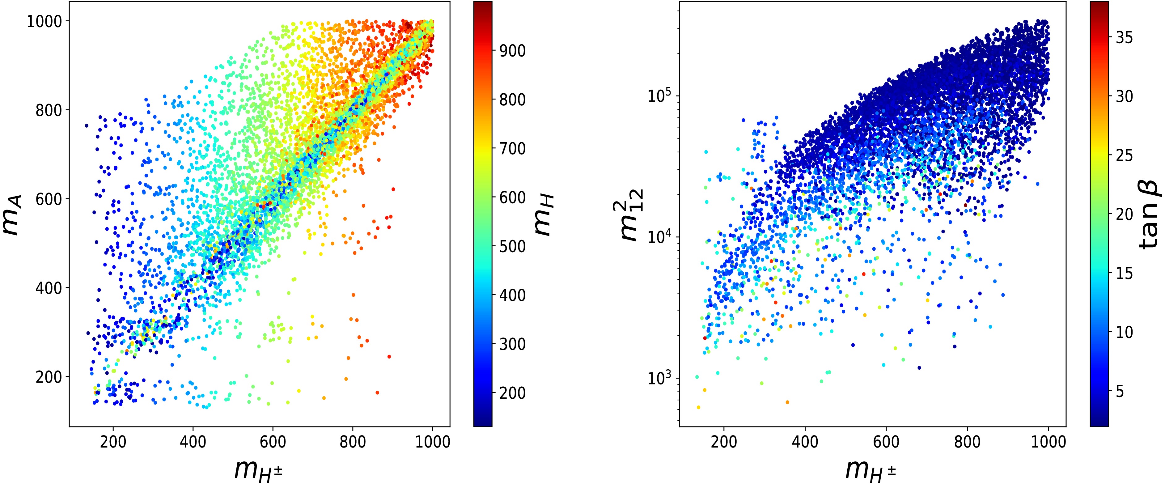
Figure 1. (color online) Scatter plots showing correlations in the parameter space:
$ (m_A,\, m_{H^\pm},\, m_H) $ in the left panel and$ (m_{12}^2,\, m_{H^\pm},\, t_{\beta}) $ in the right panel. -
A detailed review of THDM can be found in Ref. [53]. It is shown that tree-level flavor-changing neutral currents can be prevented by applying a discrete
$ Z_{2} $ symmetry in the Lagrangian, as discussed in Ref. [53]. The different charge quantum numbers of the$ Z_{2} $ for scalar doublets and fermion fields lead to four distinct Yukawa types (known as Type-I, II, X, Y) (see also Ref. [54] for more detail). The Yukawa Lagrangian can be parameterized as$ \begin{aligned}[b] {{\cal{L}}}_\text{Y} =\;& -\sum\limits_{f=u,d,\ell} \left( \sum\limits_{\phi_j=h, H} g_{\phi_j ff}\cdot \phi_j{\overline f}f + g_{Aff}\cdot A {\overline f} \gamma_5f \right) \\ & - \left[ \bar{u}_{i} \left( g_{H^+ u_i d_j}^L m_{u_i} P_L + g_{H^+ u_i d_j}^R m_{d_j} P_R \right)d_{j} H^+ \right] \\& + \cdots \end{aligned} $
(1) $ \begin{aligned}[b]\quad =\;& -\sum\limits_{f=u,d,\ell} \left( \sum\limits_{\phi_j=h, H} \frac{m_f}{v}\xi_{\phi_j}^f \phi_j {\overline f}f -{\rm i} \frac{m_f}{v}\xi_A^f {\overline f} \gamma_5fA \right)\\ & - \frac{ \sqrt{2} }{v} \left[ \bar{u}_{i} V_{ij}\left( m_{u_i} \xi^{u}_A P_L + \xi^{d}_A m_{d_j} P_R \right)d_{j} H^+ \right] \\ & - \frac{\sqrt{2}}{v} \bar{\nu}_L \xi^{\ell}_A m_\ell \ell_R H^+ + \rm{H.c}. \end{aligned} $
(2) In the Lagrangian, the CKM matrix elements are denoted by
$ V_{ij} $ ,$ \ell_{L/R} (\nu_{L/R}) $ represents the left- and right-handed lepton fields, and$ P_{L/R} = (1 \mp \gamma_{5})/2 $ denotes the projection operators. It is easy to check whether the vertices of the charged Higgs with up- and down-type quarks depend linearly on$ \cot\beta $ in the Type-X THDM. As a result, fermionic loop contributions are thus diminished in the large-$ t_{\beta} $ regime.We now turn to the theoretical and experimental bounds on THDM. Theoretical bounds are obtained by imposing conditions such as perturbative unitarity, perturbativity, and vacuum stability, all of which are taken into account in the models under consideration. In the experimental limits, the measured data of the SM-like Higgs properties, the data of flavor observables, and electroweak precision tests are taken into consideration in the constraints. We refer to our previous work [52] for further details about these conditions, wherein the Type-I THDM was studied in greater detail. The parameter space is scanned as follows. We choose parameters for the Type-X THDM within the ranges of
$ s_{\beta-\alpha} \in [0.97,1] $ ,$ t_{\beta} \in [0.5,45] $ ,$ m_{H} \in [130,1000]\; \text{GeV} $ ,$ m_{A,H^{\pm}} \in [130,1000] \; \text{GeV} $ , and$ m_{12}^2 \in [0,10^6]\; \text{GeV}^2 $ , with the SM-like Higgs mass fixed at$ m_{h} = 125.09\; \text{GeV} $ . The sampling points are first tested against theoretical constraints. The allowed points are then checked with the Electroweak Precision Observables (EWPOs). The surviving parameter space is subsequently passed to$ {\mathrm{HiggsBounds-5.10.1}}$ [55] and$ {\mathrm{HiggsSignals-2.6.1}}$ [56] to incorporate collider limits and Higgs precision measurement data, respectively. It is important to stress that both$ {\mathrm{HiggsBounds-5.10.1}}$ and$ {\mathrm{HiggsSignals-2.6.1}}$ are incorporated into$ {\mathrm{2HDMC}}$ [57]. Finally, the remaining points are evaluated with$ {\mathrm{SuperIso v4.1}}$ [58] to include flavor constraints. After all conditions are imposed, the viable parameter space is thoroughly examined as discussed below. In Fig. 1, the left panel shows the scatter plot of the viable parameter space in the$ (m_A, m_H, m_{H^\pm}) $ plane, whereas the right panel displays the scatter plot in the$ (m_{12}^2, m_{H^\pm}, t_\beta) $ plane. The results indicate that the data favor the mass region$ m_{A} > m_{H^\pm}=m_H $ over other mass patterns. Across the full charged Higgs mass range, parameter regions with$ t_{\beta}\leq 10 $ and larger$ m_{12}^2 $ values are preferred, as shown in the right panel.
Figure 1. (color online) Scatter plots showing correlations in the parameter space:
$ (m_A,\, m_{H^\pm},\, m_H) $ in the left panel and$ (m_{12}^2,\, m_{H^\pm},\, t_{\beta}) $ in the right panel. -
A detailed review of the THDM can be found in Ref. [52]. It is shown that tree-level flavor-changing neutral currents can be prevented by applying a discrete
$ Z_{2} $ symmetry in the Lagrangian, as discussed in Ref. [52]. The different charge quantum numbers of the$ Z_{2} $ for scalar doublets and fermion fields lead to four distinct Yukawa types (known as Type-I, II, X, Y) (see also Ref. [53] for more detail). The Yukawa Lagrangian can be parameterized as$ \begin{aligned}[b] {{\cal{L}}}_\text{Y} =\;& -\sum\limits_{f=u,d,\ell} \left( \sum\limits_{\phi_j=h, H} g_{\phi_j ff}\cdot \phi_j{\overline f}f + g_{Aff}\cdot A {\overline f} \gamma_5f \right) \\ & - \left[ \bar{u}_{i} \left( g_{H^+ u_i d_j}^L m_{u_i} P_L + g_{H^+ u_i d_j}^R m_{d_j} P_R \right)d_{j} H^+ \right] \\& + \cdots \end{aligned} $
(1) $ \begin{aligned}[b] =\;& -\sum\limits_{f=u,d,\ell} \left( \sum\limits_{\phi_j=h, H} \frac{m_f}{v}\xi_{\phi_j}^f \phi_j {\overline f}f -i\frac{m_f}{v}\xi_A^f {\overline f} \gamma_5fA \right)\\ & - \frac{ \sqrt{2} }{v} \left[ \bar{u}_{i} V_{ij}\left( m_{u_i} \xi^{u}_A P_L + \xi^{d}_A m_{d_j} P_R \right)d_{j} H^+ \right] \\ & - \frac{\sqrt{2}}{v} \bar{\nu}_L \xi^{\ell}_A m_\ell \ell_R H^+ + \rm{H.c}. \end{aligned} $
(2) In the Lagrangian, the CKM matrix elements are denoted by
$ V_{ij} $ ,$ \ell_{L/R} (\nu_{L/R}) $ stand for the left- and right-handed lepton fields, and$ P_{L/R} = (1 \mp \gamma_{5})/2 $ denotes the projection operators. It is easy to check that the vertices of the charged Higgs with up- and down-type quarks depend linearly on$ \cot\beta $ in the Type-X THDM. As a result, fermionic loop contributions are thus diminished in the large-$ t_{\beta} $ regime.We now turn to the theoretical and experimental bounds on the THDM, which are discussed in the following paragraphs. Theoretical bounds are obtained by imposing conditions such as perturbative unitarity, perturbativity, and vacuum stability, all of which are taken into account for the models under consideration. In the experimental limits, the measured data of the SM-like Higgs properties, the data of flavor observables, and electroweak precision tests are taken into consideration in the constraints. For explaining these conditions, we refer to our previous work [54] where Type-I THDM has been studied in further detail. The scan of the parameter space is performed as follows. We choose parameters for the Type-X THDM within the ranges of
$ s_{\beta-\alpha} \in [0.97,1] $ ,$ t_{\beta} \in [0.5,45] $ ,$ m_{H} \in [130,1000]\; \text{GeV} $ ,$ m_{A,H^{\pm}} \in [130,1000] \; \text{GeV} $ , and$ m_{12}^2 \in [0,10^6]\; \text{GeV}^2 $ , with the SM-like Higgs mass fixed at$ m_{h} = 125.09\; \text{GeV} $ . The sampling points are first tested against theoretical constraints. The allowed points are then checked with the Electroweak Precision Observables (EWPOs). The surviving parameter space is subsequently passed to$ {\mathrm{HiggsBounds-5.10.1}}$ [55] and$ {\mathrm{HiggsSignals-2.6.1}}$ [56] to incorporate collider limits and Higgs precision measurement data, respectively. It is important to stress that both$ {\mathrm{HiggsBounds-5.10.1}}$ and$ {\mathrm{HiggsSignals-2.6.1}}$ are incorporated into$ {\mathrm{2HDMC}}$ [57]. Finally, the remaining points are evaluated with$ {\mathrm{SuperIso v4.1}}$ [58] to include flavor constraints. After all conditions are imposed, the viable parameter space is thoroughly examined in the following paragraphs. In Fig. 1, the left panel shows the scatter plot of the viable parameter space in the$ (m_A, m_H, m_{H^\pm}) $ plane, while the right panel displays the scatter plot in the$ (m_{12}^2, m_{H^\pm}, t_\beta) $ plane. The results indicate that the data favor the mass region$ m_{A} > m_{H^\pm}=m_H $ over other mass patterns. Across the full charged Higgs mass range, parameter regions with$ t_{\beta}\leq 10 $ and larger$ m_{12}^2 $ values are preferred, as shown in the right panel.
Figure 1. (color online) The scatter plots show correlations in the parameter space:
$ (m_A,\, m_{H^\pm},\, m_H) $ in the left panel and$ (m_{12}^2,\, m_{H^\pm},\, t_{\beta}) $ in the right panel. -
In this work, we follow the method developed in Refs. [46, 47] and extend them for calculating the considered processes in the general
$ {\cal{R}}_{\xi} $ gauge. Furthermore, we go beyond previous works by presenting the first results verified through several self-consistency checks, such as those of ξ-independence, renormalization-scale stability, and the ultraviolet finiteness of the amplitude. As shown in Refs. [46, 47], all one-loop Feynman diagrams for this decay process in the 't Hooft–Feynman gauge are taken into account in the decay rate, and the effects of renormalization schemes on the obtained results are negligible. Thus, the effects of renormalization schemes are also neglected in this work.First, all one-loop Feynman diagrams are generated in the general
$ R_{\xi} $ gauge and are shown explicitly in Appendix C. The decay amplitude for$ H^{\pm}(p) \to W^{\pm}_{\mu}(p_{1}) Z_{\nu}(p_{2}) $ can be expressed via the form factors$ {\cal{T}}_i $ ($ i = 1,2,3 $ ) following the corresponding Lorentz structures.$ {\cal{M}}_{H^{\pm} \rightarrow W^{\pm} Z} = \Big[ g^{\mu\nu} {\cal{T}}_1 + p_2^{\mu} \, p_1^{\nu} {\cal{T}}_2 + {\rm i} \, \epsilon^{\mu\nu\rho\sigma} p_{1, \rho} \, p_{2, \sigma} \, {\cal{T}}_3 \Big] \varepsilon^{*}_{\mu} (p_1) \varepsilon^{*}_{\nu} (p_2). $
(3) where
$ \epsilon^{\mu\nu\rho\sigma} $ is the completely antisymmetric tensor, p ($ p_1 $ and$ p_2 $ ) is the ingoing (outgoing) momentum, and$ \varepsilon^{*}_{\mu} $ ($ \varepsilon^{*}_{\nu} $ ) are the polarization vectors for external$ W^\pm $ and Z bosons, respectively. In the above formulas, two relations for on-shell vector bosons$ p_1^{\mu} \varepsilon^{*}_{\mu} (p_1) = p_2^{\nu} \varepsilon^{*}_{\nu} (p_2) = 0 $ have been utilized for our calculations.The corresponding form factors
$ {\cal{T}}_i $ are decomposed into one-loop fermionic ($ {\cal{T}}_i^F $ ) and bosonic ($ {\cal{T}}_i^B $ ) contributions. The factors are computed from the respective groups of Feynman diagrams as follows:$ {\cal{T}}^{(F/B)}_i = {\cal{T}}^{(F/B)}_{i, \text{Trig}} + {\cal{T}}^{(F/B)}_{i, \text{Self}} + {\cal{T}}^{(F/B)}_{i, \text{Tad}}. $
(4) The index notations
$ F/B $ indicate the corresponding contributions from fermion and boson loops. The quantities$ {\cal{T}}^{(F/B)}_{i, \text{Trig/Self/Tad}} $ are obtained from the triangle, self-energy, and tadpole Feynman diagrams, respectively.Analytical results for
$ {\cal{T}}^{(F/B)}_{i, \text{Trig/Self/Tad}} $ in the$ {\cal{R}}_{\xi} $ gauge are presented using scalar Passarino-Veltman functions (PV-functions) [59] in Appendix A, whereas analytical checks of ξ-gauge invariance are provided in Appendix B. In this section, we describe the numerical checks of the self-consistency of the one-loop form factors, including their ξ-independence, UV finiteness, and stability under variations in the renormalization scale$ \mu^2 $ . Specifically, for ξ-gauge invariance, we examine only the form factors$ {\cal{T}}^{B}_{1,2} $ arising from boson-loop contributions, where$ \xi_W $ and$ \xi_Z $ are varied in comparison with the case$ \xi_{W/Z} = 1 $ in the 't Hooft–Feynman gauge. For illustration, we adopt representative THDM parameters:$ m_{H^\pm} = m_{H} = 800\; \text{GeV} $ ,$ m_{A} = m_{H^\pm} + m_{Z} $ ,$ s_{\beta - \alpha} = 0.98 $ and the scale of the$ Z_2 $ -symmetry$ m_{12}^2 = 5\cdot 10^4\; \text{GeV}^2 $ . The results of these checks are summarized in Tables 1, 2, where$ \xi_W $ and$ \xi_Z $ are varied over wide ranges. These results demonstrate good numerical stability.$ \big( \xi_W , \xi_Z \big) $ $ (1, 1) $ $ (10, 10^2) $ $ (10^3, 10^4) $ $ \sum \limits_{\phi} {\cal{T}}^{B, \phi-A}_{1, \text{Trig}} $ $-50.72721116 + 0 \, {\rm i}$ $ -50.79862234 + 0 \, {\rm i} $ $ -51.65760847 + 0 \, {\rm i}$ $ \sum \limits_{\phi} {\cal{T}}^{B, \phi-H^\pm}_{1, \text{Trig}} $ $ 50.66247519 + 0 \,{\rm i} $ $50.66247519 + 0 \, {\rm i}$ $ 50.66247519 + 0 \, {\rm i} $ $ \sum \limits_{\phi} {\cal{T}}^{B, \phi-W^\pm}_{1, \text{Trig}} $ $ 4.197968064 -1.192202277 \, {\rm i} $ $ 3.885889625 -0.7864121884 \, {\rm i} $ $ 9.769973063 +2.88619913 \, {\rm i} $ $ \sum \limits_{\phi} {\cal{T}}^{B, \phi-Z}_{1, \text{Trig}}$ $ 0.0173173496 + 0 \, {\rm i}$ $0.3215636277 + 0 \, {\rm i} $ $1.42510883 + 0 \, {\rm i} $ $ \sum \limits_{\phi} {\cal{T}}^{B, \phi-W^\pm Z}_{1, \text{Trig}} $ $ -4.072882533 +1.271771141 \, {\rm i} $ $ -3.945505715 +0.815048537 \, {\rm i}$ $ -10.70487047 -3.318528531 \, {\rm i} $ $ {\cal{T}}^{B}_{1, \text{Self}}$ $ 69.46890566-0.023317639 \, {\rm i}$ $78.17143601 +0.027614876 \, {\rm i} $ $-30.76307909 +0.4885806253 \, {\rm i}$ $ {\cal{T}}^{B}_{1, \text{Tad}} $ $-69.69069235 + 0 \, {\rm i}$ $ -78.44135618 + 0 \,{\rm i} $ $ 31.12388118 + 0 \, {\rm i}$ $ {\cal{T}}^{B}_{1}$ in Eq. (28)$ -0.1441197805+0.0562512244 \, {\rm i}$ $ -0.1441197805 +0.0562512244 \, {\rm i}$ $ -0.1441197808 +0.0562512244 \, {\rm i} $ Table 1. Numerical checks of
$ R_\xi $ gauge invariance for the form factor$ {\cal{T}}^{B}_{1} $ in boson-loop contributions are performed by varying the$ \xi_W $ and$ \xi_Z $ values and by comparing them with the case$ \xi_{W/Z} = 1 $ in the 't Hooft–Feynman gauge. We take the THDM parameters as follows: the Higgs masses$ m_{H^\pm} = m_{H} = 800 $ GeV,$ m_{A} = m_{H^\pm} + m_{Z} $ ,$ s_{\beta - \alpha} = 0.98 $ ,$ t_{\beta} = 10 $ , and the scale of the$ Z_2 $ -symmetry$ m_{12}^2 = 5 \cdot 10^4 $ $ {\rm{GeV}}^2 $ .$ \big( \xi_W , \xi_Z \big) $ $ (1, 1) $ $ (10, 10^2) $ $ (10^3, 10^4) $ $ \sum \limits_{\phi} {\cal{T}}^{B, \phi-A}_{2, \text{Trig}} $ $\begin{array}{l} 8.875933961 \cdot 10^{-7} + 0 \, {\rm i}\end{array}$ $\begin{array}{l} 8.875933961 \cdot 10^{-7} + 0 \, {\rm i}\end{array}$ $\begin{array}{l} 8.875933958 \cdot 10^{-7} + 0 \, {\rm i}\end{array}$ $ \sum \limits_{\phi} {\cal{T}}^{B, \phi-H^\pm}_{2, \text{Trig}}$ $ \begin{array}{l}-4.259326679 \cdot 10^{-7}+ 0 \,{\rm i} \end{array}$ $ \begin{array}{l}-4.259326679 \cdot 10^{-7}+ 0 \,{\rm i} \end{array}$ $\begin{array}{l} -4.259326683 \cdot 10^{-7}+ 0 \,{\rm i} \end{array} $ $ \sum \limits_{\phi} {\cal{T}}^{B, \phi-W^\pm}_{2, \text{Trig}} $ $ \begin{array}{l}3.525339605 \cdot 10^{-7} +5.18767908 \cdot 10^{-7} \, {\rm i} \end{array}$ $ \begin{array}{l}3.525339607 \cdot 10^{-7} +5.18767908 \cdot 10^{-7} \, {\rm i}\end{array}$ $\begin{array}{l} 3.52533961 \cdot 10^{-7} +5.1876791 \cdot 10^{-7} \, {\rm i} \end{array}$ $ \sum \limits_{\phi} {\cal{T}}^{B, \phi-Z}_{2, \text{Trig}}$ $ \begin{array}{l}-7.0029171 \cdot 10^{-8} + 0 \, {\rm i} \end{array}$ $\begin{array}{l}-7.0029171 \cdot 10^{-7} + 0 \, {\rm i} \end{array}$ $ \begin{array}{l}-7.0029174 \cdot 10^{-7}+ 0 \, {\rm i} \end{array} $ $ \sum \limits_{\phi} {\cal{T}}^{B, \phi-W^\pm Z}_{2, \text{Trig}} $ $\begin{array}{l} -8.244771 \cdot 10^{-7}-4.926311 \cdot 10^{-7} \, {\rm i} \end{array}$ $ \begin{array}{l}-8.244771 \cdot 10^{-7} -4.926311 \cdot 10^{-7} \, {\rm i}\end{array}$ $\begin{array}{l} -8.244773 \cdot 10^{-7} -4.926313 \cdot 10^{-7} \, {\rm i} \end{array}$ $ {\cal{T}}^{B}_{2, \text{Self}} $ $ 0 $ $ 0 $ $ 0 $ $ {\cal{T}}^{B}_{2, \text{Tad}} $ $ 0 $ $ 0 $ $ 0 $ $ {\cal{T}}^{B}_{2} $ in Eq. (28)$ \begin{array}{l}-8.031155 \cdot 10^{-8} +2.6136808 \cdot 10^{-8} \, {\rm i} \end{array}$ $ \begin{array}{l}-8.031155 \cdot 10^{-8} +2.6136809 \cdot 10^{-8} \, {\rm i}\end{array}$ $\begin{array}{l}-8.031154 \cdot 10^{-8} +2.613682 \cdot 10^{-8} \, {\rm i} \end{array}$ Table 2. Numerical checks of
$ R_\xi $ gauge invariance for the form factor$ {\cal{T}}^{B}_{2} $ in boson-loop contributions are performed by varying the gauge parameters$ \xi_W $ and$ \xi_Z $ . We take the THDM parameters as follows: the Higgs masses$ m_{H^\pm} = m_{H} = 800 $ GeV,$ m_{A} = m_{H^\pm} + m_{Z} $ ,$ s_{\beta - \alpha} = 0.98 $ ,$ t_{\beta} = 10 $ , and the scale of the$ Z_2 $ -symmetry$ m_{12}^2 = 5 \times 10^4 $ $ {\rm{GeV}}^2 $ .We then perform numerical checks of the
$ C_{UV} $ - and$ \mu^2 $ -independence (See Appendix A for the definitions of these parameters.) for the form factors$ {\cal{T}}_i = {\cal{T}}_i^F + {\cal{T}}_i^B $ with$ i=1,2,3 $ . We note that the total one-loop form factor should be considered in these tests, with gauge parameters fixed at$ \xi_W = \xi_Z = 100 $ for example. It should also be noted that the fermion-loop contribution$ {\cal{T}}^{F}_{1} $ is evaluated in the Type-X THDM as an illustrative example. The numerical results for these tests are obtained using the same parameter point as specified above. By varying$ C_{UV} $ and$ \mu^2 $ over wide ranges, the results demonstrate good numerical stability (see Tables 3, 4, 5).$ \big( C_{UV} , \mu^2 \big) $ $ (0,1) $ $ (10^4, 10^6) $ $ (10^6, 10^8) $ $ {\cal{T}}^{B}_{1, \text{Trig}} $ $ 0.0409007639 -0.12057752761 \, {\rm i}$ $ 0.0409007639 -0.12057752761 \, {\rm i}$ $ 0.04090076301 -0.12057752761 \, {\rm i}$ $ {\cal{T}}^{B}_{1, \text{Self}} $ $ -0.9723666455 +0.1590201866 \, {\rm i}$ $ 799.5362885 +0.1590201866 \, {\rm i}$ $ 79940.92392 +0.1590201866 \, {\rm i}$ $ {\cal{T}}^{B}_{1, \text{Tad}} $ $ 1.0786977518+ 0 \, {\rm i} $ $ -799.4299574 + 0 \,{\rm i}$ $ -79940.81759 + 0 \, {\rm i}$ $ {\cal{T}}^{B}_{1} $ $ 0.1472318702 +0.03844265898 \,{\rm i}$ $ 0.1472318702+0.03844265898 \, {\rm i} $ $ 0.1472318695+0.03844265898 \, {\rm i} $ $ {\cal{T}}^{F}_{1, \text{Trig}} $ $ 0.4996708114-0.19005144066 \, {\rm i} $ $ -497.4139502 -0.19005144066 \, {\rm i}$ $ -49723.08395 -0.19005144066 \, {\rm i}$ $ {\cal{T}}^{F}_{1, \text{Self}} $ $ -0.3824890675+0.12113853706 \, {\rm i} $ $ 375.5060921 +0.12113853706 \, {\rm i}$ $ 37537.3078+0.12113853706 \, {\rm i} $ $ {\cal{T}}^{F}_{1, \text{Tad}} $ $ -0.1133787187 + 0 \, {\rm i}$ $ 121.9116612 + 0 \, {\rm i}$ $ 12185.77995 + 0 \, {\rm i}$ $ {\cal{T}}^{F}_{1} $ $ 0.00380302517 -0.06891290359 \, {\rm i}$ $ 0.00380302517-0.06891290359 \, {\rm i} $ $ 0.00380302519-0.06891290359 \, {\rm i} $ $ {\cal{T}}_1={\cal{T}}_1^F + {\cal{T}}_1^B $ $ 0.1510348954-0.0304702446 \, {\rm i} $ $ 0.1510348954 -0.0304702446 \, {\rm i}$ $ 0.1510348947-0.0304702446 \, {\rm i} $ Table 3. Numerical checks of
$ C_{UV} $ and the renormalization scale$ \mu^2 $ are performed for the form factors$ {\cal{T}}_1 = {\cal{T}}_1^F + {\cal{T}}_1^B $ . The bosonic contribution$ {\cal{T}}^{B}_{1} $ is evaluated at$ \xi_W = \xi_Z = 100 $ , while the fermionic contribution$ {\cal{T}}^{F}_{1} $ is calculated in the Type-X THDM. For this analysis, we adopt the following set of THDM parameters:$ m_{H^\pm} = m_{H} = 500\; \text{GeV},\; m_{A} = m_{H^\pm} + m_{Z}, \; s_{\beta - \alpha} = 0.98, \; t_{\beta} = 5, \; m_{12}^2 = 5 \times 10^4\; \text{GeV}^2 $ .$ \big( C_{UV} , \mu^2 \big) $ $ (0,1) $ $ (10^4, 10^6) $ $ (10^6, 10^8) $ $ {\cal{T}}^{B}_{2, \text{Self}} $ $ 0 $ $ 0 $ $ 0 $ $ {\cal{T}}^{B}_{2, \text{Tad}} $ $ 0 $ $ 0 $ $ 0 $ $ {\cal{T}}^{B}_{2} \equiv {\cal{T}}^{B}_{2, \text{Trig}} $ $ -4.46523589 \cdot 10^{-7} +8.283757782 \cdot 10^{-8} \, {\rm i}$ $ -4.46523589 \cdot 10^{-7} +8.283757782 \cdot 10^{-8} \,{\rm i}$ $ -4.465235912 \cdot 10^{-7} +8.283757782 \cdot 10^{-8} \,{\rm i}$ $ {\cal{T}}^{F}_{2, \text{Self}} $ $ 0 $ $ 0 $ $ 0 $ $ {\cal{T}}^{F}_{2, \text{Tad}} $ $ 0 $ $ 0 $ $ 0 $ $ {\cal{T}}^{F}_{2} $ $ 1.039941873 \cdot 10^{-7}+1.445658912 \cdot 10^{-6} \, {\rm i} $ $ 1.039941873 \cdot 10^{-7}+1.445658912 \cdot 10^{-6} \, {\rm i} $ $ 1.039941873 \cdot 10^{-7}+1.445658912 \cdot 10^{-6} \, {\rm i} $ $ {\cal{T}}_2={\cal{T}}_2^F + {\cal{T}}_2^B $ $ -3.425294017 \cdot 10^{-7} +1.52849649 \cdot 10^{-6} \,{\rm i}$ $ -3.425294017 \cdot 10^{-7} +1.52849649 \cdot 10^{-6} \, {\rm i}$ $ -3.425294039 \cdot 10^{-7} +1.52849649 \cdot 10^{-6} \, {\rm i}$ Table 4. Numerical checks of
$ C_{UV} $ and the renormalization scale$ \mu^2 $ are performed for the form factors$ {\cal{T}}_2 = {\cal{T}}_2^F + {\cal{T}}_2^B $ . The bosonic contribution$ {\cal{T}}^{B}_{2} $ is evaluated at$ \xi_W = \xi_Z = 100 $ , while the fermionic contribution$ {\cal{T}}^{F}_{2} $ is calculated in the Type-X THDM. For this analysis, we adopt the following THDM parameters:$ m_{H^\pm} = m_{H} = 500\; \text{GeV} $ ,$ m_{A} = m_{H^\pm} + m_{Z} $ ,$ s_{\beta - \alpha} = 0.98 $ ,$ t_{\beta} = 5 $ , and$ m_{12}^2 = 5 \times 10^4\; \text{GeV}^2 $ .$ \big( C_{UV} , \mu^2 \big) $ $ (0,1) $ $ (10^4, 10^6) $ $ (10^6, 10^8) $ $ {\cal{T}}^{B}_{3} $ $ 0 $ $ 0 $ $ 0 $ $ {\cal{T}}^{F}_{3, \text{Self}} $ $ 0 $ $ 0 $ $ 0 $ $ {\cal{T}}^{F}_{3, \text{Tad}} $ $ 0 $ $ 0 $ $ 0 $ $ {\cal{T}}^{F}_{3} $ $ 3.220832776 \cdot 10^{-7}-1.274849257 \cdot 10^{-6} \,{\rm i} $ $ 3.220832776 \cdot 10^{-7} -1.274849257 \cdot 10^{-6} \, {\rm i}$ $ 3.220832777 \cdot 10^{-7}-1.274849257 \cdot 10^{-6} \, {\rm i} $ $ {\cal{T}}_3= {\cal{T}}_3^F + {\cal{T}}_3^B $ $ 3.220832776 \cdot 10^{-7}-1.274849257 \cdot 10^{-6} \, {\rm i} $ $ 3.220832776 \cdot 10^{-7} -1.274849257 \cdot 10^{-6} \,{\rm i}$ $ 3.220832777 \cdot 10^{-7} -1.274849257 \cdot 10^{-6} \, {\rm i}$ Table 5. Numerical checks of
$ C_{UV} $ and the renormalization scale$ \mu^2 $ are performed for the form factors$ {\cal{T}}_3 = {\cal{T}}_3^F + {\cal{T}}_3^B $ . The bosonic contribution$ {\cal{T}}^{B}_{3} $ is evaluated at$ \xi_W = \xi_Z = 100 $ , while the fermionic contribution$ {\cal{T}}^{F}_{3} $ is calculated in the Type-X THDM as an illustrative example of fermion couplings. For this analysis, we adopt the following THDM parameters:$ m_{H^\pm} = m_{H} = 500\; \text{GeV} $ ,$ m_{A} = m_{H^\pm} + m_{Z} $ ,$ s_{\beta - \alpha} = 0.98 $ ,$ t_{\beta} = 5 $ , and$ m_{12}^2 = 5 \times 10^4\; \text{GeV}^2 $ .After collecting all the necessary one-loop form factors and performing the self-consistency checks, the decay rates are computed in terms of these form factors.
$ \begin{aligned}[b]& \Gamma_{H^{\pm}\rightarrow W^{\pm} Z} = \frac{ \sqrt{ \Lambda (\mu_{W}, \mu_{Z}) } }{ 128 \pi \cdot m_{H^\pm}} \Big\{ 4 \big| {\cal{T}}_1 \big|^2 + m_{H^\pm}^4 \, \Lambda (\mu_{W}, \mu_{Z}) \, \big| {\cal{T}}_3 \big|^2 \\&\quad + \frac{ m_{H^\pm}^4 }{ 16 m_{W}^2 m_{Z}^2} \Big| 2 \big( 1 - \mu_{W} - \mu_{Z} \big) \, {\cal{T}}_1+ m_{H^\pm}^2 \, \Lambda (\mu_{W}, \mu_{Z}) \, {\cal{T}}_2 \Big|^2 \Big\}. \end{aligned} $
(5) The relevant kinematical variables are
$ \mu_{V} = m_{V}^2 / m_{H^\pm}^2 $ for$ V = W, Z $ , and the kinematical function$ \Lambda(x, y) $ is defined as$ \Lambda(x, y) = (1 - x - y)^2 - 4 x y $ . -
In this work, we follow the method developed in Refs. [46, 47] and extend these studies to the calculation of the considered processes in the general
$ {\cal{R}}_{\xi} $ gauge. Furthermore, we go beyond previous works by presenting the first results verified through several self-consistency checks, such as ξ-independence, renormalization-scale stability, and ultraviolet finiteness of the amplitude. As shown in Refs. [46, 47], all one-loop Feynman diagrams for this decay process in the 't Hooft–Feynman gauge are taken into account in the decay rate, and it was indicated that the effects of the renormalization schemes on the results are very small. Following this fact, the effects of renormalization schemes can also be neglected in this work.First, all one-loop Feynman diagrams are generated in the general
$ R_{\xi} $ gauge and are shown explicitly in Appendix C. The decay amplitude for$ H^{\pm}(p) \to W^{\pm}_{\mu}(p_{1}) Z_{\nu}(p_{2}) $ can be expressed via the form factors$ {\cal{T}}_i $ ($ i = 1,2,3 $ ) following the corresponding Lorentz structures:$ {\cal{M}}_{H^{\pm} \rightarrow W^{\pm} Z} = \Big[ g^{\mu\nu} {\cal{T}}_1 + p_2^{\mu} \, p_1^{\nu} {\cal{T}}_2 + i \, \epsilon^{\mu\nu\rho\sigma} p_{1, \rho} \, p_{2, \sigma} \, {\cal{T}}_3 \Big] \varepsilon^{*}_{\mu} (p_1) \varepsilon^{*}_{\nu} (p_2). $
(3) Where
$ \epsilon^{\mu\nu\rho\sigma} $ is the completely antisymmetric tensor, p ($ p_1 $ and$ p_2 $ ) is the ingoing (outgoing) momentum, and$ \varepsilon^{*}_{\mu} $ ($ \varepsilon^{*}_{\nu} $ ) are the polarization vectors for external$ W^\pm $ and Z bosons, respectively. In the above formulas, two relations for on-shell vector bosons$ p_1^{\mu} \varepsilon^{*}_{\mu} (p_1) = p_2^{\nu} \varepsilon^{*}_{\nu} (p_2) = 0 $ , have been utilized for our calculations.The corresponding form factors
$ {\cal{T}}_i $ are decomposed into one-loop fermionic ($ {\cal{T}}_i^F $ ) and bosonic ($ {\cal{T}}_i^B $ ) contributions. The factors are computed from the respective groups of Feynman diagrams as follows:$ {\cal{T}}^{(F/B)}_i = {\cal{T}}^{(F/B)}_{i, \text{Trig}} + {\cal{T}}^{(F/B)}_{i, \text{Self}} + {\cal{T}}^{(F/B)}_{i, \text{Tad}}. $
(4) The index notations
$ F/B $ indicate the corresponding contributions from fermion and boson loops. The quantities$ {\cal{T}}^{(F/B)}_{i, \text{Trig/Self/Tad}} $ are obtained from the triangle, self-energy, and tadpole Feynman diagrams, respectively.Analytical results for
$ {\cal{T}}^{(F/B)}_{i, \text{Trig/Self/Tad}} $ in the$ {\cal{R}}_{\xi} $ gauge are presented using scalar Passarino-Veltman functions (PV-functions) [59] in appendix A, while analytical checks of ξ-gauge invariance are provided in appendix B. In this section, we perform numerical checks of the self-consistency of the one-loop form factors, including their ξ-independence, UV finiteness, and stability under variations of the renormalization scale$ \mu^2 $ . Specifically, for ξ-gauge invariance we examine only the form factors$ {\cal{T}}^{B}_{1,2} $ arising from boson-loop contributions, where$ \xi_W $ and$ \xi_Z $ are varied in comparison with the case$ \xi_{W/Z} = 1 $ in the 't Hooft–Feynman gauge. For illustration, we adopt representative THDM parameters:$ m_{H^\pm} = m_{H} = 800\; \text{GeV} $ ,$ m_{A} = m_{H^\pm} + m_{Z} $ ,$ s_{\beta - \alpha} = 0.98 $ and the scale of the$ Z_2 $ -symmetry$ m_{12}^2 = 5\cdot 10^4\; \text{GeV}^2 $ . The results of these checks are summarized in Tables 1,2, where$ \xi_W $ and$ \xi_Z $ are varied over wide ranges. The results demonstrate good numerical stability.$ \big( \xi_W , \xi_Z \big) $ $ (1, 1) $ $ (10, 10^2) $ $ (10^3, 10^4) $ $ \sum \limits_{\phi} {\cal{T}}^{B, \phi-A}_{1, \text{Trig}} $ $ -50.72721116 + 0 \, i$ $ -50.79862234 + 0 \, i $ $ -51.65760847 + 0 \, i$ $ \sum \limits_{\phi} {\cal{T}}^{B, \phi-H^\pm}_{1, \text{Trig}} $ $ 50.66247519 + 0 \, i $ $50.66247519 + 0 \, i $ $ 50.66247519 + 0 \, i $ $ \sum \limits_{\phi} {\cal{T}}^{B, \phi-W^\pm}_{1, \text{Trig}} $ $ 4.197968064 -1.192202277 \, i $ $ 3.885889625 -0.7864121884 \, i $ $ 9.769973063 +2.88619913 \, i $ $ \sum \limits_{\phi} {\cal{T}}^{B, \phi-Z}_{1, \text{Trig}}$ $ 0.0173173496 + 0 \, i $ $0.3215636277 + 0 \, i $ $1.42510883 + 0 \, i $ $ \sum \limits_{\phi} {\cal{T}}^{B, \phi-W^\pm Z}_{1, \text{Trig}} $ $ -4.072882533 +1.271771141 \, i $ $ -3.945505715 +0.815048537 \, i$ $ -10.70487047 -3.318528531 \, i $ $ {\cal{T}}^{B}_{1, \text{Self}}$ $ 69.46890566-0.023317639 \, i $ $78.17143601 +0.027614876 \, i $ $-30.76307909 +0.4885806253 \, i $ $ {\cal{T}}^{B}_{1, \text{Tad}} $ $ -69.69069235 + 0 \, i $ $ -78.44135618 + 0 \, i $ $ 31.12388118 + 0 \, i $ $ {\cal{T}}^{B}_{1}$ in Eq. 28$ -0.1441197805+0.0562512244 \, i $ $ -0.1441197805 +0.0562512244 \, i $ $ -0.1441197808 +0.0562512244 \, i $ Table 1. Numerical checks of
$ R_\xi $ gauge invariance for the form factor$ {\cal{T}}^{B}_{1} $ in boson-loop contributions are performed by varying the values of$ \xi_W $ and$ \xi_Z $ and comparing them with the case$ \xi_{W/Z} = 1 $ in the 't Hooft–Feynman gauge. We take the THDM parameters as follows: the Higgs masses$ m_{H^\pm} = m_{H} = 800 $ GeV,$ m_{A} = m_{H^\pm} + m_{Z} $ ,$ s_{\beta - \alpha} = 0.98 $ ,$ t_{\beta} = 10 $ , and the scale of the$ Z_2 $ -symmetry$ m_{12}^2 = 5 \cdot 10^4 $ $ {\rm{GeV}}^2 $ .$ \big( \xi_W , \xi_Z \big) $ $ (1, 1) $ $ (10, 10^2) $ $ (10^3, 10^4) $ $ \sum \limits_{\phi} {\cal{T}}^{B, \phi-A}_{2, \text{Trig}} $ $\begin{array}{l} 8.875933961 \cdot 10^{-7} + 0 \, i\end{array}$ $\begin{array}{l} 8.875933961 \cdot 10^{-7} + 0 \, i\end{array}$ $\begin{array}{l} 8.875933958 \cdot 10^{-7} + 0 \, i\end{array}$ $ \sum \limits_{\phi} {\cal{T}}^{B, \phi-H^\pm}_{2, \text{Trig}}$ $ \begin{array}{l}-4.259326679 \cdot 10^{-7}+ 0 \, i \end{array}$ $ \begin{array}{l}-4.259326679 \cdot 10^{-7}+ 0 \, i \end{array}$ $\begin{array}{l} -4.259326683 \cdot 10^{-7}+ 0 \, i\end{array} $ $ \sum \limits_{\phi} {\cal{T}}^{B, \phi-W^\pm}_{2, \text{Trig}} $ $ \begin{array}{l}3.525339605 \cdot 10^{-7} +5.18767908 \cdot 10^{-7} \, i \end{array}$ $ \begin{array}{l}3.525339607 \cdot 10^{-7} +5.18767908 \cdot 10^{-7} \, i \end{array}$ $\begin{array}{l} 3.52533961 \cdot 10^{-7} +5.1876791 \cdot 10^{-7} \, i \end{array}$ $ \sum \limits_{\phi} {\cal{T}}^{B, \phi-Z}_{2, \text{Trig}}$ $ \begin{array}{l}-7.0029171 \cdot 10^{-8} + 0 \, i \end{array}$ $\begin{array}{l}-7.0029171 \cdot 10^{-7} + 0 \, i \end{array}$ $ \begin{array}{l}-7.0029174 \cdot 10^{-7}+ 0 \, i\end{array} $ $ \sum \limits_{\phi} {\cal{T}}^{B, \phi-W^\pm Z}_{2, \text{Trig}} $ $\begin{array}{l} -8.244771 \cdot 10^{-7}-4.926311 \cdot 10^{-7} \, i \end{array}$ $ \begin{array}{l}-8.244771 \cdot 10^{-7} -4.926311 \cdot 10^{-7} \, i\end{array}$ $\begin{array}{l} -8.244773 \cdot 10^{-7} -4.926313 \cdot 10^{-7} \, i \end{array}$ $ {\cal{T}}^{B}_{2, \text{Self}} $ $ 0 $ $ 0 $ $ 0 $ $ {\cal{T}}^{B}_{2, \text{Tad}} $ $ 0 $ $ 0 $ $ 0 $ $ {\cal{T}}^{B}_{2} $ in Eq. 29$ \begin{array}{l}-8.031155 \cdot 10^{-8} \\+2.6136808 \cdot 10^{-8} \, i \end{array}$ $ \begin{array}{l}-8.031155 \cdot 10^{-8} \\+2.6136809 \cdot 10^{-8} \, i \end{array}$ $\begin{array}{l}-8.031154 \cdot 10^{-8} \\+2.613682 \cdot 10^{-8} \, i \end{array}$ Table 2. Numerical checks of
$ R_\xi $ gauge invariance for the form factor$ {\cal{T}}^{B}_{2} $ in boson-loop contributions are performed by varying the gauge parameters$ \xi_W $ and$ \xi_Z $ . We take the THDM parameters as follows: the Higgs masses$ m_{H^\pm} = m_{H} = 800 $ GeV,$ m_{A} = m_{H^\pm} + m_{Z} $ ,$ s_{\beta - \alpha} = 0.98 $ ,$ t_{\beta} = 10 $ , and the scale of the$ Z_2 $ -symmetry$ m_{12}^2 = 5 \times 10^4 $ $ {\rm{GeV}}^2 $ .We then perform numerical checks of the
$ C_{UV} $ - and$ \mu^2 $ -independence See Appendix A for the definitions of these parameters) for the form factors$ {\cal{T}}_i = {\cal{T}}_i^F + {\cal{T}}_i^B $ with$ i=1,2,3 $ . We note that the total one-loop form factor should be considered in these tests, with gauge parameters fixed at$ \xi_W = \xi_Z = 100 $ for example. It should also be noted that the fermion-loop contribution$ {\cal{T}}^{F}_{1} $ is evaluated in the Type-X THDM as an illustrative example. The numerical results for these tests are obtained using the same parameter point as specified above. By varying$ C_{UV} $ and$ \mu^2 $ over wide ranges, the results demonstrate good numerical stability (see Tables 3, 4, 5).$ \big( C_{UV} , \mu^2 \big) $ $ (0,1) $ $ (10^4, 10^6) $ $ (10^6, 10^8) $ $ {\cal{T}}^{B}_{1, \text{Trig}} $ $ 0.0409007639 $ $ 0.0409007639 $ $ 0.04090076301 $ $ -0.12057752761 \, i $ $ -0.12057752761 \, i $ $ -0.12057752761 \, i $ $ {\cal{T}}^{B}_{1, \text{Self}} $ $ -0.9723666455 $ $ 799.5362885 $ $ 79940.92392 $ $ +0.1590201866 \, i $ $ +0.1590201866 \, i $ $ +0.1590201866 \, i $ $ {\cal{T}}^{B}_{1, \text{Tad}} $ $ 1.0786977518 $ $ -799.4299574 $ $ -79940.81759 $ $ + 0 \, i $ $ + 0 \, i $ $ + 0 \, i $ $ {\cal{T}}^{B}_{1} $ $ 0.1472318702 $ $ 0.1472318702 $ $ 0.1472318695 $ $ +0.03844265898 \, i $ $ +0.03844265898 \, i $ $ +0.03844265898 \, i $ $ {\cal{T}}^{F}_{1, \text{Trig}} $ $ 0.4996708114 $ $ -497.4139502 $ $ -49723.08395 $ $ -0.19005144066 \, i $ $ -0.19005144066 \, i $ $ -0.19005144066 \, i $ $ {\cal{T}}^{F}_{1, \text{Self}} $ $ -0.3824890675 $ $ 375.5060921 $ $ 37537.3078 $ $ +0.12113853706 \, i $ $ +0.12113853706 \, i $ $ +0.12113853706 \, i $ $ {\cal{T}}^{F}_{1, \text{Tad}} $ $ -0.1133787187 $ $ 121.9116612 $ $ 12185.77995 $ $ + 0 \, i $ $ + 0 \, i $ $ + 0 \, i $ $ {\cal{T}}^{F}_{1} $ $ 0.00380302517 $ $ 0.00380302517 $ $ 0.00380302519 $ $ -0.06891290359 \, i $ $ -0.06891290359 \, i $ $ -0.06891290359 \, i $ $ {\cal{T}}_1={\cal{T}}_1^F + {\cal{T}}_1^B $ $ 0.1510348954 $ $ 0.1510348954 $ $ 0.1510348947 $ $ -0.0304702446 \, i $ $ -0.0304702446 \, i $ $ -0.0304702446 \, i $ Table 3. Numerical checks of
$ C_{UV} $ and the renormalization scale$ \mu^2 $ are performed for the form factors$ {\cal{T}}_1 = {\cal{T}}_1^F + {\cal{T}}_1^B $ . The bosonic contribution$ {\cal{T}}^{B}_{1} $ is evaluated at$ \xi_W = \xi_Z = 100 $ , while the fermionic contribution$ {\cal{T}}^{F}_{1} $ is calculated in the Type-X THDM. For this analysis, we adopt the following set of THDM parameters:$ m_{H^\pm} = m_{H} = 500\; \text{GeV},\; m_{A} = m_{H^\pm} + m_{Z}, \; s_{\beta - \alpha} = 0.98, \; t_{\beta} = 5, \; m_{12}^2 = 5 \times 10^4\; \text{GeV}^2 $ .$ \big( C_{UV} , \mu^2 \big) $ $ (0,1) $ $ (10^4, 10^6) $ $ (10^6, 10^8) $ $ {\cal{T}}^{B}_{2, \text{Self}} $ $ 0 $ $ 0 $ $ 0 $ $ {\cal{T}}^{B}_{2, \text{Tad}} $ $ 0 $ $ 0 $ $ 0 $ $ {\cal{T}}^{B}_{2} \equiv {\cal{T}}^{B}_{2, \text{Trig}} $ $ -4.46523589 \cdot 10^{-7} $ $ -4.46523589 \cdot 10^{-7} $ $ -4.465235912 \cdot 10^{-7} $ $ +8.283757782 \cdot 10^{-8} \, i $ $ +8.283757782 \cdot 10^{-8} \, i $ $ +8.283757782 \cdot 10^{-8} \, i $ $ {\cal{T}}^{F}_{2, \text{Self}} $ $ 0 $ $ 0 $ $ 0 $ $ {\cal{T}}^{F}_{2, \text{Tad}} $ $ 0 $ $ 0 $ $ 0 $ $ {\cal{T}}^{F}_{2} $ $ 1.039941873 \cdot 10^{-7} $ $ 1.039941873 \cdot 10^{-7} $ $ 1.039941873 \cdot 10^{-7} $ $ +1.445658912 \cdot 10^{-6} \, i $ $ +1.445658912 \cdot 10^{-6} \, i $ $ +1.445658912 \cdot 10^{-6} \, i $ $ {\cal{T}}_2={\cal{T}}_2^F + {\cal{T}}_2^B $ $ -3.425294017 \cdot 10^{-7} $ $ -3.425294017 \cdot 10^{-7} $ $ -3.425294039 \cdot 10^{-7} $ $ +1.52849649 \cdot 10^{-6} \, i $ $ +1.52849649 \cdot 10^{-6} \, i $ $ +1.52849649 \cdot 10^{-6} \, i $ Table 4. Numerical checks of
$ C_{UV} $ and the renormalization scale$ \mu^2 $ are performed for the form factors$ {\cal{T}}_2 = {\cal{T}}_2^F + {\cal{T}}_2^B $ . The bosonic contribution$ {\cal{T}}^{B}_{2} $ is evaluated at$ \xi_W = \xi_Z = 100 $ , while the fermionic contribution$ {\cal{T}}^{F}_{2} $ is calculated in the Type-X THDM. For this analysis, we adopt the following THDM parameters:$ m_{H^\pm} = m_{H} = 500\; \text{GeV} $ ,$ m_{A} = m_{H^\pm} + m_{Z} $ ,$ s_{\beta - \alpha} = 0.98 $ ,$ t_{\beta} = 5 $ , and$ m_{12}^2 = 5 \times 10^4\; \text{GeV}^2 $ .$ \big( C_{UV} , \mu^2 \big) $ $ (0,1) $ $ (10^4, 10^6) $ $ (10^6, 10^8) $ $ {\cal{T}}^{B}_{3} $ $ 0 $ $ 0 $ $ 0 $ $ {\cal{T}}^{F}_{3, \text{Self}} $ $ 0 $ $ 0 $ $ 0 $ $ {\cal{T}}^{F}_{3, \text{Tad}} $ $ 0 $ $ 0 $ $ 0 $ $ {\cal{T}}^{F}_{3} $ $ 3.220832776 \cdot 10^{-7} $ $ 3.220832776 \cdot 10^{-7} $ $ 3.220832777 \cdot 10^{-7} $ $ -1.274849257 \cdot 10^{-6} \, i $ $ -1.274849257 \cdot 10^{-6} \, i $ $ -1.274849257 \cdot 10^{-6} \, i $ $ {\cal{T}}_3= {\cal{T}}_3^F + {\cal{T}}_3^B $ $ 3.220832776 \cdot 10^{-7} $ $ 3.220832776 \cdot 10^{-7} $ $ 3.220832777 \cdot 10^{-7} $ $ -1.274849257 \cdot 10^{-6} \, i $ $ -1.274849257 \cdot 10^{-6} \, i $ $ -1.274849257 \cdot 10^{-6} \, i $ Table 5. Numerical checks of
$ C_{UV} $ and the renormalization scale$ \mu^2 $ are performed for the form factors$ {\cal{T}}_3 = {\cal{T}}_3^F + {\cal{T}}_3^B $ . The bosonic contribution$ {\cal{T}}^{B}_{3} $ is evaluated at$ \xi_W = \xi_Z = 100 $ , while the fermionic contribution$ {\cal{T}}^{F}_{3} $ is calculated in the Type-X THDM as an illustrative example of fermion couplings. For this analysis, we adopt the following THDM parameters:$ m_{H^\pm} = m_{H} = 500\; \text{GeV} $ ,$ m_{A} = m_{H^\pm} + m_{Z} $ ,$ s_{\beta - \alpha} = 0.98 $ ,$ t_{\beta} = 5 $ , and$ m_{12}^2 = 5 \times 10^4\; \text{GeV}^2 $ .After collecting all the necessary one-loop form factors and performing the self-consistency checks, the decay rates are computed in terms of these form factors as follows:
$ \begin{aligned}[b] \Gamma_{H^{\pm}\rightarrow W^{\pm} Z} =\;& \frac{ \sqrt{ \Lambda (\mu_{W}, \mu_{Z}) } }{ 128 \pi \cdot m_{H^\pm}} \Big\{ 4 \big| {\cal{T}}_1 \big|^2 + m_{H^\pm}^4 \, \Lambda (\mu_{W}, \mu_{Z}) \, \big| {\cal{T}}_3 \big|^2 \\&+ \frac{ m_{H^\pm}^4 }{ 16 m_{W}^2 m_{Z}^2} \Big| 2 \big( 1 - \mu_{W} - \mu_{Z} \big) \, {\cal{T}}_1\\& + m_{H^\pm}^2 \, \Lambda (\mu_{W}, \mu_{Z}) \, {\cal{T}}_2 \Big|^2 \Big\}. \end{aligned} $
(5) The relevant kinematical variables are
$ \mu_{V} = m_{V}^2 / m_{H^\pm}^2 $ for$ V = W, Z $ , and the kinematical function$ \Lambda(x, y) $ is defined as follows$ \Lambda(x, y) = (1 - x - y)^2 - 4 x y $ . -
Singly charged Higgs boson production at muon–TeV colliders is investigated in this section. For the phenomenological analysis, we use the following benchmark configuration:
$ s_{\beta-\alpha} = 0.98 $ ,$ m_{A} = m_{H^\pm}+m_Z = m_H + m_Z $ , and$ m_{12}^2 = 5\times 10^{4}\; \text{GeV}^2 $ . The charged Higgs mass is scanned over the range$ 200\; \text{GeV} \leq m_{H^\pm} \leq 1000\; \text{GeV} $ , whereas while the mixing parameter is set as$ 2 \leq t_{\beta} \leq 12 $ . All other SM parameters are taken from the Particle Data Group [60]. -
Singly charged Higgs boson production at muon–TeV colliders is investigated in this section. For the phenomenological analysis, we use the following benchmark configuration:
$ s_{\beta-\alpha} = 0.98 $ ,$ m_{A} = m_{H^\pm}+m_Z = m_H + m_Z $ , and$ m_{12}^2 = 5\cdot 10^{4}\; \text{GeV}^2 $ . The charged Higgs mass is scanned over the range$ 200\; \text{GeV} \leq m_{H^\pm} \leq 1000\; \text{GeV} $ , while the mixing parameter is chosen as$ 2 \leq t_{\beta} \leq 12 $ . All other SM parameters are taken from the Particle Data Group [60]. -
Singly charged Higgs boson production at muon–TeV colliders is investigated in this section. For the phenomenological analysis, we use the following benchmark configuration:
$ s_{\beta-\alpha} = 0.98 $ ,$ m_{A} = m_{H^\pm}+m_Z = m_H + m_Z $ , and$ m_{12}^2 = 5\times 10^{4}\; \text{GeV}^2 $ . The charged Higgs mass is scanned over the range$ 200\; \text{GeV} \leq m_{H^\pm} \leq 1000\; \text{GeV} $ , whereas while the mixing parameter is set as$ 2 \leq t_{\beta} \leq 12 $ . All other SM parameters are taken from the Particle Data Group [60]. -
We first evaluate the branching fractions of the charged Higgs boson in the Type-X THDM. The one-loop–induced process
$ H^{\pm} \rightarrow W^\pm \gamma $ has already been reported in our previous work [52], whereas decay mode$ H^{\pm} \rightarrow W^\pm Z $ is considered in this work. The remaining decay channels are taken from Ref. [48]. In Fig. 2, the branching fractions of the charged Higgs boson are shown for all considered decay modes within the interval$ 200\; \text{GeV} \leq m_{H^\pm} \leq 1000\; \text{GeV} $ . At$ t_{\beta}=2 $ , the$ tb $ and$ Wh $ channels are the leading contributions, whereas the branching ratio of$ H^{\pm} \rightarrow W^\pm Z $ remains of the order$ 10^{-4} $ across the entire mass range. For$ t_{\beta}=4 $ , the$ tb $ and$ Wh $ channels continue to dominate; however, the$ H^{\pm} \rightarrow W^\pm Z $ mode remains around$ \sim 10^{-4} $ . Next, we consider the branching fractions at$ t_{\beta}=8 $ . We find that the branching ratio of$ H^{\pm} \rightarrow W^\pm Z $ increases to the order of$ 10^{-2} $ in the low-mass region but decreases to about$ 10^{-3} $ at higher masses. Finally, we examine the case of$ t_{\beta}=12 $ . The results show that the$ H^{\pm} \rightarrow W^\pm Z $ branching ratio can reach the order of$ 10^{-1} $ in the low-mass region, whereas it remains at the level of$ 10^{-4} $ for larger charged Higgs masses. As indicated in the previous section, the fermionic-loop contributions are suppressed in the high-$ t_{\beta} $ regime. The interference between the fermionic- and bosonic-loop contributions is small and has the opposite sign compared with the squared bosonic contributions. As a result, the decay rates of the$ H^{\pm} \rightarrow W^\pm Z $ mode are enhanced in the high-$ t_{\beta} $ region compared with the small-$ t_{\beta} $ regime.
Figure 2. (color online) Charged Higgs decay branching ratios in the Type-X THDM are shown for the benchmark scenario described above. Each plot is shown for
$ t_{\beta} = 2 $ (top left),$ t_{\beta} = 4 $ (top right),$ t_{\beta} = 8 $ (bottom left), and$ t_{\beta} = 12 $ (bottom right). -
We first evaluate the branching fractions of the charged Higgs boson in the Type-X THDM. The one-loop–induced process
$ H^{\pm} \rightarrow W^\pm \gamma $ has already been reported in our previous work [54] while decay mode$ H^{\pm} \rightarrow W^\pm Z $ is devoted in this work. The remaining decay channels are taken from [48]. In Fig. 2, the branching fractions of the charged Higgs boson are shown for all considered decay modes within the interval$ 200\; \text{GeV} \leq m_{H^\pm} \leq 1000\; \text{GeV} $ . At$ t_{\beta}=2 $ , the$ tb $ and$ Wh $ channels are the leading contributions, whereas the branching ratio of$ H^{\pm} \rightarrow W^\pm Z $ remains of the order$ 10^{-4} $ across the entire mass range. For$ t_{\beta}=4 $ , the$ tb $ and$ Wh $ channels continue to dominate, while the$ H^{\pm} \rightarrow W^\pm Z $ mode stays around$ \sim 10^{-4} $ . Next, we consider the branching fractions at$ t_{\beta}=8 $ . We find that the branching ratio of$ H^{\pm} \rightarrow W^\pm Z $ increases to the order of$ 10^{-2} $ in the low-mass region but decreases to about$ 10^{-3} $ at higher masses. Finally, we examine the case of$ t_{\beta}=12 $ . The results show that the$ H^{\pm} \rightarrow W^\pm Z $ branching ratio can reach the order of$ 10^{-1} $ in the low-mass region, while it remains at the level of$ 10^{-4} $ for larger charged Higgs masses. As indicated in the previous section, the fermionic-loop contributions are suppressed in the high-$ t_{\beta} $ regime. The interference between the fermionic-loop and bosonic-loop contributions is small and has the opposite sign compared with the squared bosonic contributions. As a result, this leads to the enhanced decay rates of the$ H^{\pm} \rightarrow W^\pm Z $ mode in the high-$ t_{\beta} $ region compared with the small-$ t_{\beta} $ regime.
Figure 2. (color online) The charged Higgs decay branching ratios in the Type-X THDM are shown for the benchmark scenario described above. Each plot is shown for
$ t_{\beta} = 2 $ (top left),$ t_{\beta} = 4 $ (top right),$ t_{\beta} = 8 $ (bottom left), and$ t_{\beta} = 12 $ (bottom right). -
We first evaluate the branching fractions of the charged Higgs boson in the Type-X THDM. The one-loop–induced process
$ H^{\pm} \rightarrow W^\pm \gamma $ has already been reported in our previous work [52], whereas decay mode$ H^{\pm} \rightarrow W^\pm Z $ is considered in this work. The remaining decay channels are taken from Ref. [48]. In Fig. 2, the branching fractions of the charged Higgs boson are shown for all considered decay modes within the interval$ 200\; \text{GeV} \leq m_{H^\pm} \leq 1000\; \text{GeV} $ . At$ t_{\beta}=2 $ , the$ tb $ and$ Wh $ channels are the leading contributions, whereas the branching ratio of$ H^{\pm} \rightarrow W^\pm Z $ remains of the order$ 10^{-4} $ across the entire mass range. For$ t_{\beta}=4 $ , the$ tb $ and$ Wh $ channels continue to dominate; however, the$ H^{\pm} \rightarrow W^\pm Z $ mode remains around$ \sim 10^{-4} $ . Next, we consider the branching fractions at$ t_{\beta}=8 $ . We find that the branching ratio of$ H^{\pm} \rightarrow W^\pm Z $ increases to the order of$ 10^{-2} $ in the low-mass region but decreases to about$ 10^{-3} $ at higher masses. Finally, we examine the case of$ t_{\beta}=12 $ . The results show that the$ H^{\pm} \rightarrow W^\pm Z $ branching ratio can reach the order of$ 10^{-1} $ in the low-mass region, whereas it remains at the level of$ 10^{-4} $ for larger charged Higgs masses. As indicated in the previous section, the fermionic-loop contributions are suppressed in the high-$ t_{\beta} $ regime. The interference between the fermionic- and bosonic-loop contributions is small and has the opposite sign compared with the squared bosonic contributions. As a result, the decay rates of the$ H^{\pm} \rightarrow W^\pm Z $ mode are enhanced in the high-$ t_{\beta} $ region compared with the small-$ t_{\beta} $ regime.
Figure 2. (color online) Charged Higgs decay branching ratios in the Type-X THDM are shown for the benchmark scenario described above. Each plot is shown for
$ t_{\beta} = 2 $ (top left),$ t_{\beta} = 4 $ (top right),$ t_{\beta} = 8 $ (bottom left), and$ t_{\beta} = 12 $ (bottom right). -
We first evaluate the branching fractions of the charged Higgs boson in the Type-X THDM. The one-loop–induced process
$ H^{\pm} \rightarrow W^\pm \gamma $ has already been reported in our previous work [52], whereas decay mode$ H^{\pm} \rightarrow W^\pm Z $ is considered in this work. The remaining decay channels are taken from Ref. [48]. In Fig. 2, the branching fractions of the charged Higgs boson are shown for all considered decay modes within the interval$ 200\; \text{GeV} \leq m_{H^\pm} \leq 1000\; \text{GeV} $ . At$ t_{\beta}=2 $ , the$ tb $ and$ Wh $ channels are the leading contributions, whereas the branching ratio of$ H^{\pm} \rightarrow W^\pm Z $ remains of the order$ 10^{-4} $ across the entire mass range. For$ t_{\beta}=4 $ , the$ tb $ and$ Wh $ channels continue to dominate; however, the$ H^{\pm} \rightarrow W^\pm Z $ mode remains around$ \sim 10^{-4} $ . Next, we consider the branching fractions at$ t_{\beta}=8 $ . We find that the branching ratio of$ H^{\pm} \rightarrow W^\pm Z $ increases to the order of$ 10^{-2} $ in the low-mass region but decreases to about$ 10^{-3} $ at higher masses. Finally, we examine the case of$ t_{\beta}=12 $ . The results show that the$ H^{\pm} \rightarrow W^\pm Z $ branching ratio can reach the order of$ 10^{-1} $ in the low-mass region, whereas it remains at the level of$ 10^{-4} $ for larger charged Higgs masses. As indicated in the previous section, the fermionic-loop contributions are suppressed in the high-$ t_{\beta} $ regime. The interference between the fermionic- and bosonic-loop contributions is small and has the opposite sign compared with the squared bosonic contributions. As a result, the decay rates of the$ H^{\pm} \rightarrow W^\pm Z $ mode are enhanced in the high-$ t_{\beta} $ region compared with the small-$ t_{\beta} $ regime.
Figure 2. (color online) Charged Higgs decay branching ratios in the Type-X THDM are shown for the benchmark scenario described above. Each plot is shown for
$ t_{\beta} = 2 $ (top left),$ t_{\beta} = 4 $ (top right),$ t_{\beta} = 8 $ (bottom left), and$ t_{\beta} = 12 $ (bottom right). -
We investigate the potential to probe charged Higgs pair production by analyzing the process
$ \mu^+\mu^- \rightarrow H^{+}H^{-} \rightarrow W^{\pm}W^{\mp}Zh $ at muon–TeV colliders. It is well known that initial-state radiation (ISR) effects play a crucial role at future lepton colliders. These effects must be taken into account to simulate the signals of the charged Higgs as well to evaluate the corresponding SM backgrounds. By applying the factorization theorems for soft and collinear singularities, the ISR contributions to charged Higgs pair production can be calculated using the master formula$ {\rm d}\sigma (s) = \int {\rm d} x_1 {\rm d} x_2 D(x_1, s) D(x_2, s) {\rm d}\sigma_0 (x_1 x_2 s) \Theta ( \rm{cuts}). $
(6) In Eq. (6),
${\rm d}\sigma_0$ denotes tree-level differential cross sections for both signals$ \mu^-\mu^+ \to H^\pm H^\mp \to W^{\pm}W^{\mp}Zh $ and the SM background process$ \mu^-\mu^+ \to W^{\pm}W^{\mp}Zh $ . All tree-level Feynman diagrams for the process$ \mu^-\mu^+ \to H^\pm H^\mp $ within THDM are shown in Fig. D1. The partonic cross sections are computed by using$ { {\mathrm{FeynArts/FormCalc}}}$ [61].$ \Theta ( \rm{cuts}) $ represents the appropriate cuts applied in the simulation, as described explicitly in the following paragraphs.$ D(x_2, s) $ is the structure function (SF). Of note, we use the SF functions from Ref. [62], which were originally applied for electron beams. However, at high-energy regions operating at muon–TeV colliders, these SF functions could also be applied to muon beams. For this reason, we apply the SF functions from Ref. [62] with$ m_{\ell} = m_{\mu} $ appropriately. The expressions for the SF functions are presented in the following paragraphs. The all-order SF functions, which are valid in the soft-photon limit, are given by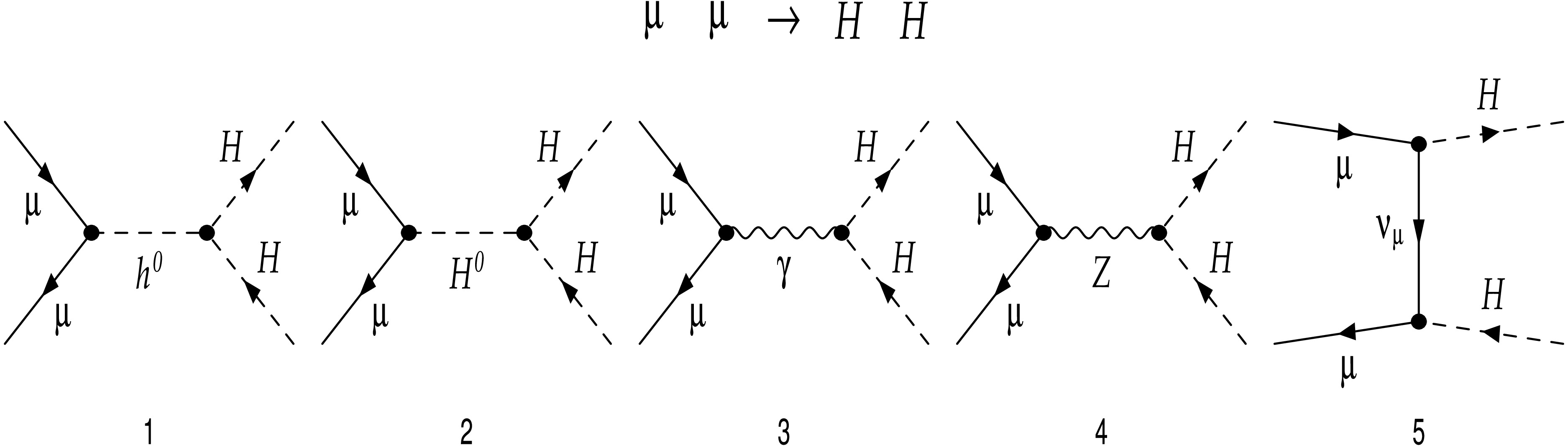
Figure D1. Feynman diagrams for
$ \mu^+\mu^- \rightarrow H^{+}H^{-} $ are generated by$ {\mathrm{FeynArts}}$ [61].$ D_{GL} (x,s ) = \frac{\exp\left[ \dfrac{1}{2} \beta \left( \dfrac{3}{4} - \gamma_E \right) \right]}{\Gamma \left( 1 + \dfrac{1}{2} \beta \right) } \frac{1}{2} \beta \left( 1 - x \right)^{\frac{1}{2} \beta - 1}, $
(7) where
$ \beta = \frac{2 \alpha}{\pi} (L - 1), \quad L = \ln(s/m_{\ell}^2). $
(8) Here, α is the fine-structure constant, and
$ m_{\ell} $ denotes the lepton mass. The symbol Γ represents the Gamma function, and$ \gamma_E $ is the Euler–Mascheroni constant. Photon radiation can be considered in the collinear approximation and through collinear logarithmic enhancements, which are included in the large-β factor. According to Eq. (7), the additive SF function up to third-order expansion terms is expressed as follows [62].$ \begin{aligned}[b] D_A (x,s) =\;& D_{GL} (x,s) - \frac{1}{4} \beta (1+x) + \frac{1}{32} \beta^2 \left[ \left(1+x \right) \left(-4 \ln (1-x) + 3 \ln(x) \right) -4 \frac{\ln x}{1-x} -5 -x \right] \\& + \frac{1}{384} \beta^3 \Bigg\{ (1+x) \left[ 18 \zeta(2) -6 {\rm Li}_2 (x) -12 \ln^2 (1-x) \right] + \frac{1}{1-x} \left[ - \frac{3}{2} (1 + 8 x + 3 x^2) \ln x -6 (x+5) (1-x) \ln(1-x) \right. \\&-12 (1+x^2) \ln x \ln(1-x) + \frac{1}{2} (1+7 x^2) \ln^2 x - \left. \frac{1}{4} (39 - 24 x - 15 x^2) \right] \Bigg\}. \end{aligned} $
(9) In this structure function, the Riemann ζ function is taken into account and
$ {\rm Li}_2 $ is the dilogarithm functions. Furthermore, the factorized SF function up to third order expansion terms can be obtained as [63, 64]$ \begin{aligned}[b] D_F (x,s) =\;& D_{GL} (x,s) \\& \times \Bigg\{ \frac{1}{2} (1 + x^2) - \frac{\beta}{16} \left[ (1 + 3 x^2) \ln x + 2(1-x)^2 \right] \\ & + \frac{\beta^2}{32} \Big[ (1-x)^2 + \frac{1}{2} (3x^2 - 4x+1) \ln x \\ & + \frac{1}{12} (1+7x^2) \ln^2 x + (1-x^2) {\rm Li}_2 (1-x) \Big] \Bigg\}. \end{aligned} $
(10) In this work, we consider the ISR effects for both the signal and the SM background processes. The effects of ISR on the scattering process
$ \mu^+\mu^- \rightarrow H^{+}H^{-} \rightarrow W^{\pm}W^{\mp}Zh $ are examined as functions of the center-of-mass energy (left panel) and of the charged Higgs mass at$ \sqrt{s}=3 $ TeV (right panel). In the left plot, we vary the center-of-mass energy from$ 1000 $ GeV to$ 5000 $ GeV and fix$ m_{H^\pm}=300 $ GeV with$ t_\beta=8 $ . We find that the ISR corrections change from approximately$ -40 $ % to$ -20 $ %. For the plot shown in the panel at right, we examine the ISR corrections at$ \sqrt{s}=3000 $ GeV while varying the charged Higgs mass and fixing$ t_\beta=8 $ . The results indicate that the corrections range from$ -20 $ % to$ -30 $ % for charged Higgs masses in the interval$ [300,600] $ GeV. In Fig. 3,$\sigma_{\rm ISR1}$ ($\sigma_{\rm ISR2}$ ) denotes the cross-section calculated using the structure functions from Eqs. (9) and (10).
Figure 3. (color online) Effects of ISR on the scattering process
$ \mu^+\mu^- \rightarrow H^{+}H^{-} \rightarrow W^{\pm}W^{\mp}Zh $ are examined as functions of the center-of-mass energy (left panel) and of the charged Higgs mass at$ \sqrt{s}=3 $ TeV (right panel).Using the cross section with ISR corrections, we evaluate the signal events for
$ \mu^+\mu^- \rightarrow H^{+}H^{-} \rightarrow W^{\pm}W^{\mp}Zh $ at$ \sqrt{s}=3 $ TeV and the integrated luminosity of$ 3000 $ fb–1. The events are generated in the parameter space of$ m_{H^\pm} $ and the mixing angle$ t_{\beta} $ as shown in Fig. 4. In this study, we vary$ 300\; \text{GeV} \leq m_{H^\pm} \leq 600\; \text{GeV} $ and$ 2 \leq t_{\beta} \leq 12 $ . The results indicate that the signal events are significant in regions of low charged Higgs masses and large$ t_{\beta} $ values, while in other regions the events become negligible. In the right-panel plot of Fig. 4, the significance of the signals relative to the SM backgrounds is presented at$ {\cal{L}}=500 $ fb–1. While the corresponding signal significances are presented at$ {\cal{L}}=1000 $ fb–1 in the left and at$ {\cal{L}}=3000 $ fb–1 in the right panel of Fig. 5. The SM background is calculated using the$ {\mathrm{GRACE}}$ program [65]. It is emphasized that the SM background also includes the ISR corrections in the evaluation of the significance. To reduce the SM background, we apply cuts on the invariant masses of the final-state particles:$ |m_{Wh}-m_{H^\pm}| \lt 10 $ GeV and$ |m_{WZ}-m_{H^\pm}| \lt 10 $ GeV. The significances are shown for$ t_{\beta}=2 $ (green points),$ t_{\beta}=4 $ (yellow points),$ t_{\beta}=8 $ (blue points), and$ t_{\beta}=12 $ (black points). Our results indicate that in the low-mass regions of the charged Higgs, and for$ t_{\beta}=8 $ and$ 10 $ , the significances can exceed$ 5\sigma $ , while in other regions they become negligible.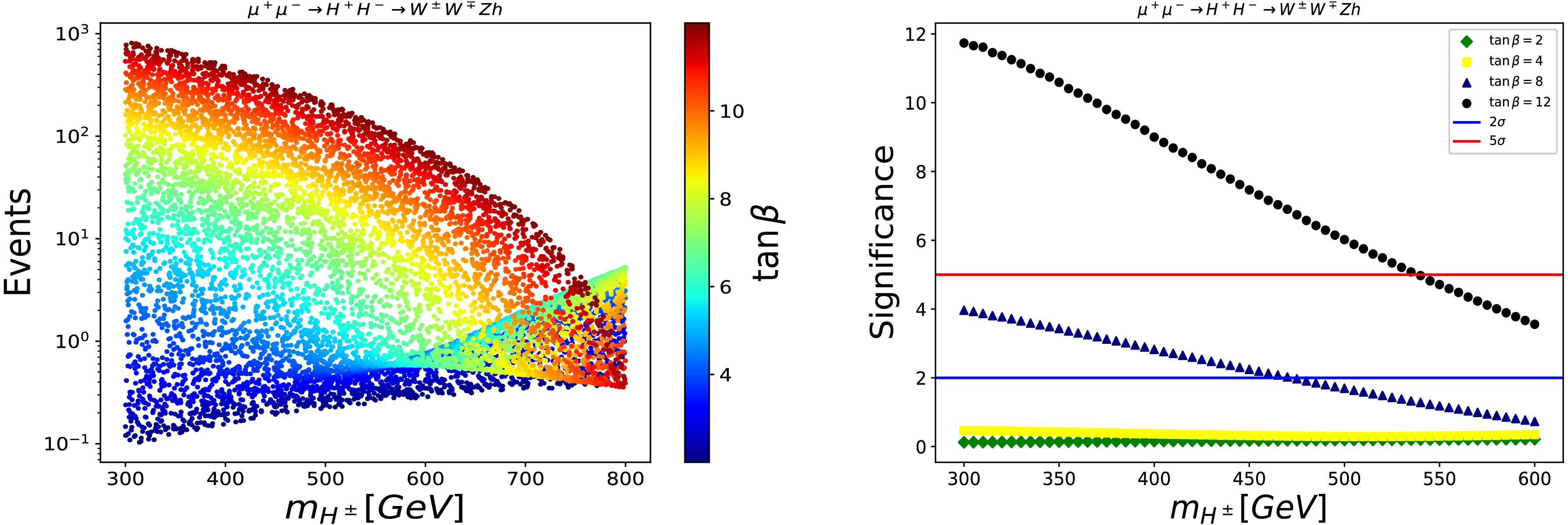
Figure 4. (color online) Event distributions of the process
$ \mu^+\mu^- \rightarrow H^{+}H^{-} \rightarrow W^{\pm}W^{\mp}Zh $ at an integrated luminosity of$ {\cal{L}}=3000\; \text{fb}^{-1} $ including ISR corrections are shown in the left panel. The corresponding signal significance taking into account the Standard Model backgrounds is presented at$ {\cal{L}}=500\; \text{fb}^{-1} $ in the right panel.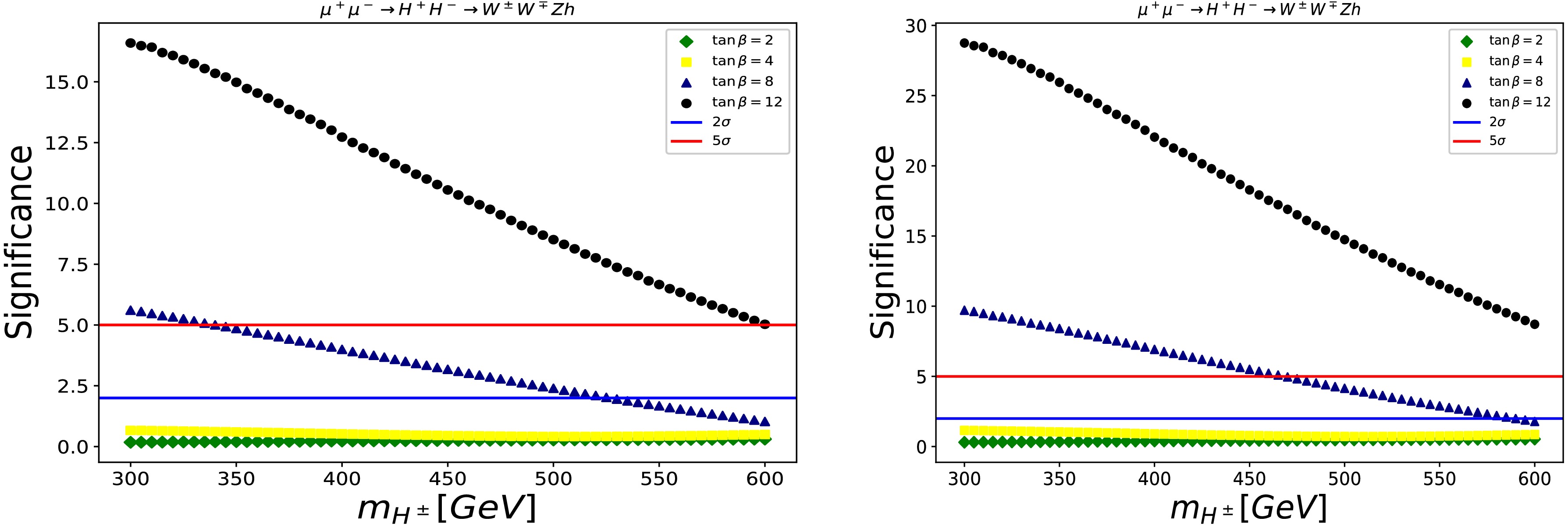
Figure 5. (color online) The corresponding signal significance taking into account the Standard Model backgrounds, is presented at
$ {\cal{L}}=1000 $ fb–1 in the left and at$ {\cal{L}}=3000 $ fb–1 in the right panel.Serveral useful points on the systematic uncertainties that might affect the significance are discussed in the following paragraphs. It is well known that the one-loop electroweak radiative corrections to the processes
$ \mu^+\mu^- \rightarrow H^{+}H^{-} \rightarrow W^{\pm}W^{\mp}Zh $ and$ \mu^+\mu^- \rightarrow W^{\pm}W^{\mp}Zh $ can be estimated from the enhancement contributions of the single Sudakov logarithm [66].$ \delta_{W} \sim -\frac{\alpha(M_Z^2)}{\pi \sin^2\theta_W} \log \left(\frac{s}{M_Z^2}\right) \sim {\cal{O}}(-10\%) \quad \text{at } \sqrt{s} = 3\; \text{TeV}. $
(11) If weak and ISR corrections are included in the significance calculation, the total electroweak correction can reach approximately
$ {\cal{O}} $ (–35%). All theoretical uncertainties and detector effects can be incorporated into the systematic uncertainty fraction of the background yield, denoted by$ \varepsilon_B $ . Consequently, the significance is modified as$ {\cal{S}} = \frac{N_{ \rm{S}}} {\sqrt{N_{ \rm{S}} + \varepsilon_B N_{ \rm{B}}}}. $
(12) For example, by taking
$ \varepsilon_B = 1.3 $ and$ \varepsilon_B = 1.5 $ , we verfy wherher the significances vary only slightly due to the small SM background after applying the effective cuts described above. Finally, if we consider the decays$ W \to \ell \nu_{\ell} $ for$ \ell = e, \mu, \tau $ with branching fractions of$ 0.3272 $ ,$ Z \to b\bar{b} $ with a branching fraction of$ 0.1512 $ , and$ h \to b\bar{b} $ with a branching fraction of$ 0.53 $ from the Particle Data Group [60], the significances are subsequently scaled down by a factor of$ 0.161927 $ , which reduces them to around$ 5\sigma $ at an integrated luminosity of$ {\cal{L}} = 3000\; \text{fb}^{-1} $ for the low-mass regions. Details of detector simulations, b-tagging, etc. will be addressed in our future work. -
We investigate the potential to probe charged Higgs pair production by analyzing the process
$ \mu^+\mu^- \rightarrow H^{+}H^{-} \rightarrow W^{\pm}W^{\mp}Zh $ at muon–TeV colliders. It is well known that initial-state radiation (ISR) effects play a crucial role at future lepton colliders. These effects must be taken into account to simulate the signals of the charged Higgs as well to evaluate the corresponding SM backgrounds. By applying the factorization theorems for soft and collinear singularities, the ISR contributions to charged Higgs pair production can be calculated using the master formula$ {\rm d}\sigma (s) = \int {\rm d} x_1 {\rm d} x_2 D(x_1, s) D(x_2, s) {\rm d}\sigma_0 (x_1 x_2 s) \Theta ( \rm{cuts}). $
(6) In Eq. (6),
${\rm d}\sigma_0$ denotes tree-level differential cross sections for both signals$ \mu^-\mu^+ \to H^\pm H^\mp \to W^{\pm}W^{\mp}Zh $ and the SM background process$ \mu^-\mu^+ \to W^{\pm}W^{\mp}Zh $ . All tree-level Feynman diagrams for the process$ \mu^-\mu^+ \to H^\pm H^\mp $ within THDM are shown in Fig. D1. The partonic cross sections are computed by using$ { {\mathrm{FeynArts/FormCalc}}}$ [61].$ \Theta ( \rm{cuts}) $ represents the appropriate cuts applied in the simulation, as described explicitly in the following paragraphs.$ D(x_2, s) $ is the structure function (SF). Of note, we use the SF functions from Ref. [62], which were originally applied for electron beams. However, at high-energy regions operating at muon–TeV colliders, these SF functions could also be applied to muon beams. For this reason, we apply the SF functions from Ref. [62] with$ m_{\ell} = m_{\mu} $ appropriately. The expressions for the SF functions are presented in the following paragraphs. The all-order SF functions, which are valid in the soft-photon limit, are given by
Figure D1. Feynman diagrams for
$ \mu^+\mu^- \rightarrow H^{+}H^{-} $ are generated by$ {\mathrm{FeynArts}}$ [61].$ D_{GL} (x,s ) = \frac{\exp\left[ \dfrac{1}{2} \beta \left( \dfrac{3}{4} - \gamma_E \right) \right]}{\Gamma \left( 1 + \dfrac{1}{2} \beta \right) } \frac{1}{2} \beta \left( 1 - x \right)^{\frac{1}{2} \beta - 1}, $
(7) where
$ \beta = \frac{2 \alpha}{\pi} (L - 1), \quad L = \ln(s/m_{\ell}^2). $
(8) Here, α is the fine-structure constant, and
$ m_{\ell} $ denotes the lepton mass. The symbol Γ represents the Gamma function, and$ \gamma_E $ is the Euler–Mascheroni constant. Photon radiation can be considered in the collinear approximation and through collinear logarithmic enhancements, which are included in the large-β factor. According to Eq. (7), the additive SF function up to third-order expansion terms is expressed as follows [62].$ \begin{aligned}[b] D_A (x,s) =\;& D_{GL} (x,s) - \frac{1}{4} \beta (1+x) + \frac{1}{32} \beta^2 \left[ \left(1+x \right) \left(-4 \ln (1-x) + 3 \ln(x) \right) -4 \frac{\ln x}{1-x} -5 -x \right] \\& + \frac{1}{384} \beta^3 \Bigg\{ (1+x) \left[ 18 \zeta(2) -6 {\rm Li}_2 (x) -12 \ln^2 (1-x) \right] + \frac{1}{1-x} \left[ - \frac{3}{2} (1 + 8 x + 3 x^2) \ln x -6 (x+5) (1-x) \ln(1-x) \right. \\&-12 (1+x^2) \ln x \ln(1-x) + \frac{1}{2} (1+7 x^2) \ln^2 x - \left. \frac{1}{4} (39 - 24 x - 15 x^2) \right] \Bigg\}. \end{aligned} $
(9) In this structure function, the Riemann ζ function is taken into account and
$ {\rm Li}_2 $ is the dilogarithm functions. Furthermore, the factorized SF function up to third order expansion terms can be obtained as [63, 64]$ \begin{aligned}[b] D_F (x,s) =\;& D_{GL} (x,s) \\& \times \Bigg\{ \frac{1}{2} (1 + x^2) - \frac{\beta}{16} \left[ (1 + 3 x^2) \ln x + 2(1-x)^2 \right] \\ & + \frac{\beta^2}{32} \Big[ (1-x)^2 + \frac{1}{2} (3x^2 - 4x+1) \ln x \\ & + \frac{1}{12} (1+7x^2) \ln^2 x + (1-x^2) {\rm Li}_2 (1-x) \Big] \Bigg\}. \end{aligned} $
(10) In this work, we consider the ISR effects for both the signal and the SM background processes. The effects of ISR on the scattering process
$ \mu^+\mu^- \rightarrow H^{+}H^{-} \rightarrow W^{\pm}W^{\mp}Zh $ are examined as functions of the center-of-mass energy (left panel) and of the charged Higgs mass at$ \sqrt{s}=3 $ TeV (right panel). In the left plot, we vary the center-of-mass energy from$ 1000 $ GeV to$ 5000 $ GeV and fix$ m_{H^\pm}=300 $ GeV with$ t_\beta=8 $ . We find that the ISR corrections change from approximately$ -40 $ % to$ -20 $ %. For the plot shown in the panel at right, we examine the ISR corrections at$ \sqrt{s}=3000 $ GeV while varying the charged Higgs mass and fixing$ t_\beta=8 $ . The results indicate that the corrections range from$ -20 $ % to$ -30 $ % for charged Higgs masses in the interval$ [300,600] $ GeV. In Fig. 3,$\sigma_{\rm ISR1}$ ($\sigma_{\rm ISR2}$ ) denotes the cross-section calculated using the structure functions from Eqs. (9) and (10).
Figure 3. (color online) Effects of ISR on the scattering process
$ \mu^+\mu^- \rightarrow H^{+}H^{-} \rightarrow W^{\pm}W^{\mp}Zh $ are examined as functions of the center-of-mass energy (left panel) and of the charged Higgs mass at$ \sqrt{s}=3 $ TeV (right panel).Using the cross section with ISR corrections, we evaluate the signal events for
$ \mu^+\mu^- \rightarrow H^{+}H^{-} \rightarrow W^{\pm}W^{\mp}Zh $ at$ \sqrt{s}=3 $ TeV and the integrated luminosity of$ 3000 $ fb–1. The events are generated in the parameter space of$ m_{H^\pm} $ and the mixing angle$ t_{\beta} $ as shown in Fig. 4. In this study, we vary$ 300\; \text{GeV} \leq m_{H^\pm} \leq 600\; \text{GeV} $ and$ 2 \leq t_{\beta} \leq 12 $ . The results indicate that the signal events are significant in regions of low charged Higgs masses and large$ t_{\beta} $ values, while in other regions the events become negligible. In the right-panel plot of Fig. 4, the significance of the signals relative to the SM backgrounds is presented at$ {\cal{L}}=500 $ fb–1. While the corresponding signal significances are presented at$ {\cal{L}}=1000 $ fb–1 in the left and at$ {\cal{L}}=3000 $ fb–1 in the right panel of Fig. 5. The SM background is calculated using the$ {\mathrm{GRACE}}$ program [65]. It is emphasized that the SM background also includes the ISR corrections in the evaluation of the significance. To reduce the SM background, we apply cuts on the invariant masses of the final-state particles:$ |m_{Wh}-m_{H^\pm}| < 10 $ GeV and$ |m_{WZ}-m_{H^\pm}| < 10 $ GeV. The significances are shown for$ t_{\beta}=2 $ (green points),$ t_{\beta}=4 $ (yellow points),$ t_{\beta}=8 $ (blue points), and$ t_{\beta}=12 $ (black points). Our results indicate that in the low-mass regions of the charged Higgs, and for$ t_{\beta}=8 $ and$ 10 $ , the significances can exceed$ 5\sigma $ , while in other regions they become negligible.
Figure 4. (color online) Event distributions of the process
$ \mu^+\mu^- \rightarrow H^{+}H^{-} \rightarrow W^{\pm}W^{\mp}Zh $ at an integrated luminosity of$ {\cal{L}}=3000\; \text{fb}^{-1} $ including ISR corrections are shown in the left panel. The corresponding signal significance taking into account the Standard Model backgrounds is presented at$ {\cal{L}}=500\; \text{fb}^{-1} $ in the right panel.
Figure 5. (color online) The corresponding signal significance taking into account the Standard Model backgrounds, is presented at
$ {\cal{L}}=1000 $ fb–1 in the left and at$ {\cal{L}}=3000 $ fb–1 in the right panel.Serveral useful points on the systematic uncertainties that might affect the significance are discussed in the following paragraphs. It is well known that the one-loop electroweak radiative corrections to the processes
$ \mu^+\mu^- \rightarrow H^{+}H^{-} \rightarrow W^{\pm}W^{\mp}Zh $ and$ \mu^+\mu^- \rightarrow W^{\pm}W^{\mp}Zh $ can be estimated from the enhancement contributions of the single Sudakov logarithm [66].$ \delta_{W} \sim -\frac{\alpha(M_Z^2)}{\pi \sin^2\theta_W} \log \left(\frac{s}{M_Z^2}\right) \sim {\cal{O}}(-10\%) \quad \text{at } \sqrt{s} = 3\; \text{TeV}. $
(11) If weak and ISR corrections are included in the significance calculation, the total electroweak correction can reach approximately
$ {\cal{O}} $ (–35%). All theoretical uncertainties and detector effects can be incorporated into the systematic uncertainty fraction of the background yield, denoted by$ \varepsilon_B $ . Consequently, the significance is modified as$ {\cal{S}} = \frac{N_{ \rm{S}}} {\sqrt{N_{ \rm{S}} + \varepsilon_B N_{ \rm{B}}}}. $
(12) For example, by taking
$ \varepsilon_B = 1.3 $ and$ \varepsilon_B = 1.5 $ , we verfy wherher the significances vary only slightly due to the small SM background after applying the effective cuts described above. Finally, if we consider the decays$ W \to \ell \nu_{\ell} $ for$ \ell = e, \mu, \tau $ with branching fractions of$ 0.3272 $ ,$ Z \to b\bar{b} $ with a branching fraction of$ 0.1512 $ , and$ h \to b\bar{b} $ with a branching fraction of$ 0.53 $ from the Particle Data Group [60], the significances are subsequently scaled down by a factor of$ 0.161927 $ , which reduces them to around$ 5\sigma $ at an integrated luminosity of$ {\cal{L}} = 3000\; \text{fb}^{-1} $ for the low-mass regions. Details of detector simulations, b-tagging, etc. will be addressed in our future work. -
We investigate the potential to probe charged Higgs pair production by analyzing the process
$ \mu^+\mu^- \rightarrow H^{+}H^{-} \rightarrow W^{\pm}W^{\mp}Zh $ at muon–TeV colliders. It is well known that initial-state radiation (ISR) effects play a crucial role at future lepton colliders. These effects must be taken into account for simulating the signals of the charged Higgs as well as evaluating the corresponding SM backgrounds. By applying the factorization theorems for soft and collinear singularities, the ISR contributions to charged Higgs pair production can be calculated as the following master formula:$ d\sigma (s) = \int d x_1 d x_2 D(x_1, s) D(x_2, s) d\sigma_0 (x_1 x_2 s) \Theta ( \rm{cuts}). $
(6) In Eq. (6),
$ d\sigma_0 $ denotes for tree-level differential cross sections for both signals$ \mu^-\mu^+ \to H^\pm H^\mp \to W^{\pm}W^{\mp}Zh $ and the SM background process$ \mu^-\mu^+ \to W^{\pm}W^{\mp}Zh $ . All tree-level Feynman diagrams for the process$ \mu^-\mu^+ \to H^\pm H^\mp $ within the THDM are shown in Fig. D1. The partonic cross-sections are computed by using the computer tools$ { {\mathrm{FeynArts/FormCalc}}}$ [68]. Additionally,$ \Theta ( \rm{cuts}) $ represents the appropriate cuts applied in the simulation, as shown explicitly in the following paragraphs.$ D(x_2, s) $ is the structure function (SF). It is noted that we use the SF functions from Ref. [61], which were originally applied for electron beams. However, at high-energy regions operating at muon–TeV colliders, these SF functions could also be applicable for muon beams. For this reason, we apply the SF functions from Ref. [61] with$ m_{\ell} = m_{\mu} $ appropriately. The explicit expressions for the SF functions are presented in the following paragraphs. The all-order SF functions, which are valid in the soft-photon limit, are given by:
Figure D1. Feynman diagrams for
$ \mu^+\mu^- \rightarrow H^{+}H^{-} $ are generated by$ {\mathrm{FeynArts}}$ [68].$ D_{GL} (x,s ) = \frac{\exp\left[ \dfrac{1}{2} \beta \left( \dfrac{3}{4} - \gamma_E \right) \right]}{\Gamma \left( 1 + \dfrac{1}{2} \beta \right) } \frac{1}{2} \beta \left( 1 - x \right)^{\frac{1}{2} \beta - 1}, $
(7) where
$ \beta = \frac{2 \alpha}{\pi} (L - 1), \quad L = \ln(s/m_{\ell}^2). $
(8) Here, α is the fine-structure constant, and
$ m_{\ell} $ denotes the lepton mass. The symbol Γ represents the Gamma function, and$ \gamma_E $ is the Euler–Mascheroni constant. Photon radiation can be treated in the collinear approximation and through collinear logarithmic enhancements, which are included in the large-β factor. According to Eq. (7), the additive SF function up to third-order expansion terms is expressed as follows [61]:$ \begin{aligned}[b] D_A (x,s) =\;& D_{GL} (x,s) - \frac{1}{4} \beta (1+x) + \frac{1}{32} \beta^2 \left[ \left(1+x \right) \left(-4 \ln (1-x) + 3 \ln(x) \right) -4 \frac{\ln x}{1-x} -5 -x \right] \\& + \frac{1}{384} \beta^3 \Bigg\{ (1+x) \left[ 18 \zeta(2) -6 {\rm Li}_2 (x) -12 \ln^2 (1-x) \right] + \frac{1}{1-x} \left[ - \frac{3}{2} (1 + 8 x + 3 x^2) \ln x -6 (x+5) (1-x) \ln(1-x) \right. \\&-12 (1+x^2) \ln x \ln(1-x) + \frac{1}{2} (1+7 x^2) \ln^2 x - \left. \frac{1}{4} (39 - 24 x - 15 x^2) \right] \Bigg\}. \end{aligned} $
(9) In this structure function, the Riemann ζ function is taken into account and
$ {\rm Li}_2 $ is the dilogarithm functions. Furthermore, the factorized SF function up to third order expansion terms can be obtained as [62, 63]:$ \begin{aligned}[b] D_F (x,s) =\;& D_{GL} (x,s) \\& \times \Bigg\{ \frac{1}{2} (1 + x^2) - \frac{\beta}{16} \left[ (1 + 3 x^2) \ln x + 2(1-x)^2 \right] \\ & + \frac{\beta^2}{32} \Big[ (1-x)^2 + \frac{1}{2} (3x^2 - 4x+1) \ln x \\ & + \frac{1}{12} (1+7x^2) \ln^2 x + (1-x^2) {\rm Li}_2 (1-x) \Big] \Bigg\}. \end{aligned} $
(10) In this work, we consider the ISR effects for both the signal and the SM background processes. The effects of ISR on the scattering process
$ \mu^+\mu^- \rightarrow H^{+}H^{-} \rightarrow W^{\pm}W^{\mp}Zh $ are examined as functions of the center-of-mass energy (left panel) and of the charged Higgs mass at$ \sqrt{s}=3 $ TeV (right panel). In the left plot, we vary the center-of-mass energy from$ 1000 $ GeV to$ 5000 $ GeV and fix$ m_{H^\pm}=300 $ GeV with$ t_\beta=8 $ . We find that the ISR corrections change from approximately$ -40 $ % to$ -20 $ %. For the right-panel plot, we study the ISR corrections at$ \sqrt{s}=3000 $ GeV while varying the charged Higgs mass and fixing$ t_\beta=8 $ . The results indicate that the corrections are from$ -20 $ % to$ -30 $ % for charged Higgs masses in the interval$ [300,600] $ GeV. In Fig. 3,$ \sigma_{ISR1} $ ($ \sigma_{ISR2} $ ) denotes the cross section calculated using the structure functions from Eqs. 9 and 10.
Figure 3. (color online) The effects of ISR on the scattering process
$ \mu^+\mu^- \rightarrow H^{+}H^{-} \rightarrow W^{\pm}W^{\mp}Zh $ are examined as functions of the center-of-mass energy (left panel) and of the charged Higgs mass at$ \sqrt{s}=3 $ TeV (right panel).Using the cross section with ISR corrections, we evaluate the signal events for
$ \mu^+\mu^- \rightarrow H^{+}H^{-} \rightarrow W^{\pm}W^{\mp}Zh $ at$ \sqrt{s}=3 $ TeV and the integrated luminosity of$ 3000 $ fb-1. The events are generated in the parameter space of$ m_{H^\pm} $ and the mixing angle$ t_{\beta} $ as shown in Fig. 4. In this study, we vary$ 300\; \text{GeV} \leq m_{H^\pm} \leq 600\; \text{GeV} $ and$ 2 \leq t_{\beta} \leq 12 $ . The results indicate that the signal events are significant in regions of low charged Higgs masses and large$ t_{\beta} $ values, while in other regions the events become negligible. In the right-panel plot of Fig. 4, the significance of the signals relative to the SM backgrounds is presented at$ {\cal{L}}=500 $ fb-1. While the corresponding signal significances are presented at$ {\cal{L}}=1000 $ fb-1 in the left and at$ {\cal{L}}=3000 $ fb-1 in the right panel of Fig. 5. The SM background is calculated using the$ {\mathrm{GRACE}}$ program [64]. It is emphasized that the SM background also includes the ISR corrections in the evaluation of the significance. To reduce the SM background, we apply cuts on the invariant masses of the final-state particles:$ |m_{Wh}-m_{H^\pm}| < 10 $ GeV and$ |m_{WZ}-m_{H^\pm}| < 10 $ GeV. The significances are shown for$ t_{\beta}=2 $ (green points),$ t_{\beta}=4 $ (yellow points),$ t_{\beta}=8 $ (blue points), and$ t_{\beta}=12 $ (black points). Our results indicate that in the low-mass regions of the charged Higgs, and for$ t_{\beta}=8 $ and$ 10 $ , the significances can exceed$ 5\sigma $ , while in other regions they become negligible.
Figure 4. (color online) The event distributions of the process
$ \mu^+\mu^- \rightarrow H^{+}H^{-} \rightarrow W^{\pm}W^{\mp}Zh $ at an integrated luminosity of$ {\cal{L}}=3000\; \text{fb}^{-1} $ , including ISR corrections, are shown in the left panel. The corresponding signal significance taking into account the Standard Model backgrounds, is presented at$ {\cal{L}}=500\; \text{fb}^{-1} $ in the right panel.
Figure 5. (color online) The corresponding signal significance taking into account the Standard Model backgrounds, is presented at
$ {\cal{L}}=1000 $ fb-1 in the left and at$ {\cal{L}}=3000 $ fb-1 in the right panel.Serveral useful comments on the systematic uncertainties that might affect the significance, are discussed in the following paragraphs. It is well known that the one-loop electroweak radiative corrections to the processes
$ \mu^+\mu^- \rightarrow H^{+}H^{-} \rightarrow W^{\pm}W^{\mp}Zh $ and$ \mu^+\mu^- \rightarrow W^{\pm}W^{\mp}Zh $ can be estimated from the enhancement contributions of the single Sudakov logarithm [69]:$ \delta_{W} \sim -\frac{\alpha(M_Z^2)}{\pi \sin^2\theta_W} \log \left(\frac{s}{M_Z^2}\right) \sim {\cal{O}}(-10\%) \quad \text{at } \sqrt{s} = 3\; \text{TeV}. $
(11) If weak and ISR corrections are included in the significance calculation, the total electroweak correction can reach approximately
$ {\cal{O}} $ (-35%). All theoretical uncertainties and detector effects can be incorporated into the systematic uncertainty fraction of the background yield, denoted by$ \varepsilon_B $ . Consequently, the significance is modified as$ {\cal{S}} = \frac{N_{ \rm{S}}} {\sqrt{N_{ \rm{S}} + \varepsilon_B N_{ \rm{B}}}}. $
(12) For instance, by taking
$ \varepsilon_B = 1.3 $ and$ \varepsilon_B = 1.5 $ , we checked that the significances vary only slightly due to the small Standard Model background after applying the effective cuts described above. Last, if we consider the decays$ W \to \ell \nu_{\ell} $ for$ \ell = e, \mu, \tau $ with branching fractions of$ 0.3272 $ ,$ Z \to b\bar{b} $ with a branching fraction of$ 0.1512 $ , and$ h \to b\bar{b} $ with a branching fraction of$ 0.53 $ from the Particle Data Group [60], the significances are subsequently scaled down by a factor of$ 0.161927 $ , reducing them to around$ 5\sigma $ at an integrated luminosity of$ {\cal{L}} = 3000\; \text{fb}^{-1} $ for the low-mass regions. Details of detector simulations, b-tagging, etc. will be addressed in our future work. -
We investigate the potential to probe charged Higgs pair production by analyzing the process
$ \mu^+\mu^- \rightarrow H^{+}H^{-} \rightarrow W^{\pm}W^{\mp}Zh $ at muon–TeV colliders. It is well known that initial-state radiation (ISR) effects play a crucial role at future lepton colliders. These effects must be taken into account to simulate the signals of the charged Higgs as well to evaluate the corresponding SM backgrounds. By applying the factorization theorems for soft and collinear singularities, the ISR contributions to charged Higgs pair production can be calculated using the master formula$ {\rm d}\sigma (s) = \int {\rm d} x_1 {\rm d} x_2 D(x_1, s) D(x_2, s) {\rm d}\sigma_0 (x_1 x_2 s) \Theta ( \rm{cuts}). $
(6) In Eq. (6),
${\rm d}\sigma_0$ denotes tree-level differential cross sections for both signals$ \mu^-\mu^+ \to H^\pm H^\mp \to W^{\pm}W^{\mp}Zh $ and the SM background process$ \mu^-\mu^+ \to W^{\pm}W^{\mp}Zh $ . All tree-level Feynman diagrams for the process$ \mu^-\mu^+ \to H^\pm H^\mp $ within THDM are shown in Fig. D1. The partonic cross sections are computed by using$ { {\mathrm{FeynArts/FormCalc}}}$ [61].$ \Theta ( \rm{cuts}) $ represents the appropriate cuts applied in the simulation, as described explicitly in the following paragraphs.$ D(x_2, s) $ is the structure function (SF). Of note, we use the SF functions from Ref. [62], which were originally applied for electron beams. However, at high-energy regions operating at muon–TeV colliders, these SF functions could also be applied to muon beams. For this reason, we apply the SF functions from Ref. [62] with$ m_{\ell} = m_{\mu} $ appropriately. The expressions for the SF functions are presented in the following paragraphs. The all-order SF functions, which are valid in the soft-photon limit, are given by
Figure D1. Feynman diagrams for
$ \mu^+\mu^- \rightarrow H^{+}H^{-} $ are generated by$ {\mathrm{FeynArts}}$ [61].$ D_{GL} (x,s ) = \frac{\exp\left[ \dfrac{1}{2} \beta \left( \dfrac{3}{4} - \gamma_E \right) \right]}{\Gamma \left( 1 + \dfrac{1}{2} \beta \right) } \frac{1}{2} \beta \left( 1 - x \right)^{\frac{1}{2} \beta - 1}, $
(7) where
$ \beta = \frac{2 \alpha}{\pi} (L - 1), \quad L = \ln(s/m_{\ell}^2). $
(8) Here, α is the fine-structure constant, and
$ m_{\ell} $ denotes the lepton mass. The symbol Γ represents the Gamma function, and$ \gamma_E $ is the Euler–Mascheroni constant. Photon radiation can be considered in the collinear approximation and through collinear logarithmic enhancements, which are included in the large-β factor. According to Eq. (7), the additive SF function up to third-order expansion terms is expressed as follows [62].$ \begin{aligned}[b] D_A (x,s) =\;& D_{GL} (x,s) - \frac{1}{4} \beta (1+x) + \frac{1}{32} \beta^2 \left[ \left(1+x \right) \left(-4 \ln (1-x) + 3 \ln(x) \right) -4 \frac{\ln x}{1-x} -5 -x \right] \\& + \frac{1}{384} \beta^3 \Bigg\{ (1+x) \left[ 18 \zeta(2) -6 {\rm Li}_2 (x) -12 \ln^2 (1-x) \right] + \frac{1}{1-x} \left[ - \frac{3}{2} (1 + 8 x + 3 x^2) \ln x -6 (x+5) (1-x) \ln(1-x) \right. \\&-12 (1+x^2) \ln x \ln(1-x) + \frac{1}{2} (1+7 x^2) \ln^2 x - \left. \frac{1}{4} (39 - 24 x - 15 x^2) \right] \Bigg\}. \end{aligned} $
(9) In this structure function, the Riemann ζ function is taken into account and
$ {\rm Li}_2 $ is the dilogarithm functions. Furthermore, the factorized SF function up to third order expansion terms can be obtained as [63, 64]$ \begin{aligned}[b] D_F (x,s) =\;& D_{GL} (x,s) \\& \times \Bigg\{ \frac{1}{2} (1 + x^2) - \frac{\beta}{16} \left[ (1 + 3 x^2) \ln x + 2(1-x)^2 \right] \\ & + \frac{\beta^2}{32} \Big[ (1-x)^2 + \frac{1}{2} (3x^2 - 4x+1) \ln x \\ & + \frac{1}{12} (1+7x^2) \ln^2 x + (1-x^2) {\rm Li}_2 (1-x) \Big] \Bigg\}. \end{aligned} $
(10) In this work, we consider the ISR effects for both the signal and the SM background processes. The effects of ISR on the scattering process
$ \mu^+\mu^- \rightarrow H^{+}H^{-} \rightarrow W^{\pm}W^{\mp}Zh $ are examined as functions of the center-of-mass energy (left panel) and of the charged Higgs mass at$ \sqrt{s}=3 $ TeV (right panel). In the left plot, we vary the center-of-mass energy from$ 1000 $ GeV to$ 5000 $ GeV and fix$ m_{H^\pm}=300 $ GeV with$ t_\beta=8 $ . We find that the ISR corrections change from approximately$ -40 $ % to$ -20 $ %. For the plot shown in the panel at right, we examine the ISR corrections at$ \sqrt{s}=3000 $ GeV while varying the charged Higgs mass and fixing$ t_\beta=8 $ . The results indicate that the corrections range from$ -20 $ % to$ -30 $ % for charged Higgs masses in the interval$ [300,600] $ GeV. In Fig. 3,$\sigma_{\rm ISR1}$ ($\sigma_{\rm ISR2}$ ) denotes the cross-section calculated using the structure functions from Eqs. (9) and (10).
Figure 3. (color online) Effects of ISR on the scattering process
$ \mu^+\mu^- \rightarrow H^{+}H^{-} \rightarrow W^{\pm}W^{\mp}Zh $ are examined as functions of the center-of-mass energy (left panel) and of the charged Higgs mass at$ \sqrt{s}=3 $ TeV (right panel).Using the cross section with ISR corrections, we evaluate the signal events for
$ \mu^+\mu^- \rightarrow H^{+}H^{-} \rightarrow W^{\pm}W^{\mp}Zh $ at$ \sqrt{s}=3 $ TeV and the integrated luminosity of$ 3000 $ fb–1. The events are generated in the parameter space of$ m_{H^\pm} $ and the mixing angle$ t_{\beta} $ as shown in Fig. 4. In this study, we vary$ 300\; \text{GeV} \leq m_{H^\pm} \leq 600\; \text{GeV} $ and$ 2 \leq t_{\beta} \leq 12 $ . The results indicate that the signal events are significant in regions of low charged Higgs masses and large$ t_{\beta} $ values, while in other regions the events become negligible. In the right-panel plot of Fig. 4, the significance of the signals relative to the SM backgrounds is presented at$ {\cal{L}}=500 $ fb–1. While the corresponding signal significances are presented at$ {\cal{L}}=1000 $ fb–1 in the left and at$ {\cal{L}}=3000 $ fb–1 in the right panel of Fig. 5. The SM background is calculated using the$ {\mathrm{GRACE}}$ program [65]. It is emphasized that the SM background also includes the ISR corrections in the evaluation of the significance. To reduce the SM background, we apply cuts on the invariant masses of the final-state particles:$ |m_{Wh}-m_{H^\pm}| < 10 $ GeV and$ |m_{WZ}-m_{H^\pm}| < 10 $ GeV. The significances are shown for$ t_{\beta}=2 $ (green points),$ t_{\beta}=4 $ (yellow points),$ t_{\beta}=8 $ (blue points), and$ t_{\beta}=12 $ (black points). Our results indicate that in the low-mass regions of the charged Higgs, and for$ t_{\beta}=8 $ and$ 10 $ , the significances can exceed$ 5\sigma $ , while in other regions they become negligible.
Figure 4. (color online) Event distributions of the process
$ \mu^+\mu^- \rightarrow H^{+}H^{-} \rightarrow W^{\pm}W^{\mp}Zh $ at an integrated luminosity of$ {\cal{L}}=3000\; \text{fb}^{-1} $ including ISR corrections are shown in the left panel. The corresponding signal significance taking into account the Standard Model backgrounds is presented at$ {\cal{L}}=500\; \text{fb}^{-1} $ in the right panel.
Figure 5. (color online) The corresponding signal significance taking into account the Standard Model backgrounds, is presented at
$ {\cal{L}}=1000 $ fb–1 in the left and at$ {\cal{L}}=3000 $ fb–1 in the right panel.Serveral useful points on the systematic uncertainties that might affect the significance are discussed in the following paragraphs. It is well known that the one-loop electroweak radiative corrections to the processes
$ \mu^+\mu^- \rightarrow H^{+}H^{-} \rightarrow W^{\pm}W^{\mp}Zh $ and$ \mu^+\mu^- \rightarrow W^{\pm}W^{\mp}Zh $ can be estimated from the enhancement contributions of the single Sudakov logarithm [66].$ \delta_{W} \sim -\frac{\alpha(M_Z^2)}{\pi \sin^2\theta_W} \log \left(\frac{s}{M_Z^2}\right) \sim {\cal{O}}(-10\%) \quad \text{at } \sqrt{s} = 3\; \text{TeV}. $
(11) If weak and ISR corrections are included in the significance calculation, the total electroweak correction can reach approximately
$ {\cal{O}} $ (–35%). All theoretical uncertainties and detector effects can be incorporated into the systematic uncertainty fraction of the background yield, denoted by$ \varepsilon_B $ . Consequently, the significance is modified as$ {\cal{S}} = \frac{N_{ \rm{S}}} {\sqrt{N_{ \rm{S}} + \varepsilon_B N_{ \rm{B}}}}. $
(12) For example, by taking
$ \varepsilon_B = 1.3 $ and$ \varepsilon_B = 1.5 $ , we verfy wherher the significances vary only slightly due to the small SM background after applying the effective cuts described above. Finally, if we consider the decays$ W \to \ell \nu_{\ell} $ for$ \ell = e, \mu, \tau $ with branching fractions of$ 0.3272 $ ,$ Z \to b\bar{b} $ with a branching fraction of$ 0.1512 $ , and$ h \to b\bar{b} $ with a branching fraction of$ 0.53 $ from the Particle Data Group [60], the significances are subsequently scaled down by a factor of$ 0.161927 $ , which reduces them to around$ 5\sigma $ at an integrated luminosity of$ {\cal{L}} = 3000\; \text{fb}^{-1} $ for the low-mass regions. Details of detector simulations, b-tagging, etc. will be addressed in our future work. -
We now turn our attention to another process,
$ \mu^+\mu^- \rightarrow \gamma \gamma \rightarrow H^{+}H^{-} \rightarrow W^{\pm}W^{\mp}Zh $ . The total cross section is calculated by convoluting the partonic process$ \gamma \gamma \rightarrow H^{+}H^{-} \rightarrow W^{\pm}W^{\mp}Zh $ with the photon structure function as follows:$ \sigma(s) = \int_{\tfrac{2m_{H^\pm}} {\sqrt{s}}}^{x_{\text{max}}} {\rm d}z \, \left( 2z \int_{z^2/x_{\text{max}}}^{x_{\text{max}}} \frac{{\rm d}x}{x} \, f_{\gamma/\mu}(x) \, f_{\gamma/\mu} \left(z^2/x\right) \right) \, \hat{\sigma}(\hat{s} = z^2 s). $
(13) Here, the photon structure function
$ f_{\gamma/\mu}(x) $ is used, with x denoting the energy fraction of the photon emitted by the incoming lepton. The explicit formulas for$ f_{\gamma/\mu}(x) $ are given in [67] with the appropriate of$ m_{\ell}=m_{\mu} $ as in [68] for example. In the master formulas, we adopt$ x_{\rm max} = 0.83 $ as in [69]. All tree-level Feynman diagrams for the process$ \gamma \gamma \to H^\pm H^\mp $ within the THDM are shown in Fig. D2. The partonic process$ \gamma \gamma \to H^+ H^- $ are generated by FeynArts/ FormCalc [61]. The SM background which is the process$ \gamma \gamma \to W^\pm W^\mp Z h $ , is calculated using the the$ {\mathrm{GRACE}}$ program [65]. To reduce the SM background, we apply cuts on the invariant masses of the final-state particles:$ |m_{Wh}-m_{H^\pm}| \lt 10 $ GeV and and$ |m_{WZ}-m_{H^\pm}| \lt 10 $ GeV. In Fig. 6, the numbers of events of the process$ \mu^+\mu^- \to \gamma\gamma \rightarrow H^{+}H^{-} \rightarrow W^{\pm}W^{\mp}Zh $ at an integrated luminosity of$ {\cal{L}}=3000\; \text{fb}^{-1} $ are shown in the left panel of Fig. 6. The signal significances considering the Standard Model backgrounds are presented at$ {\cal{L}}=500 $ fb–1 in the right panel of Fig. 6, while the significances are presented at$ {\cal{L}}=1000 $ fb–1 on the left panel and at$ {\cal{L}}=5000 $ fb–1 on the right panel of Fig. 7. We observe that the events become significant when the charged Higgs masses are in the low-mass region and$ t_{\beta} = 8, 12 $ , whereas they are small and can be ignored in other regions. For charged Higgs masses in the low-mass region and$ t_{\beta} = 12 $ , the significance can exceed$ 5\sigma $ . In other cases, the significances are negligible.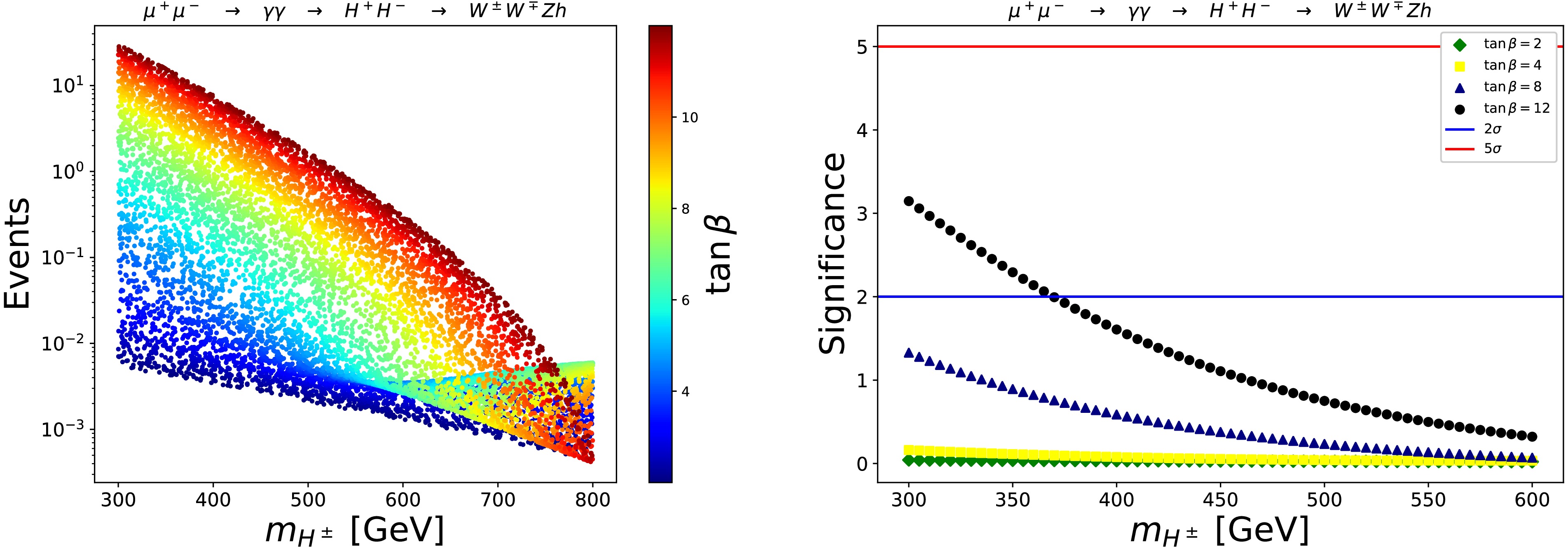
Figure 6. (color online) The signal events of the process
$ \mu^+\mu^- \to \gamma\gamma \rightarrow H^{+}H^{-} \rightarrow W^{\pm}W^{\mp}Zh $ at an integrated luminosity of$ {\cal{L}}=3000\; \text{fb}^{-1} $ are shown in the left panel. The corresponding signal significance taking into account the SM backgrounds is presented at$ {\cal{L}}=500\; \text{fb}^{-1} $ in the right panel.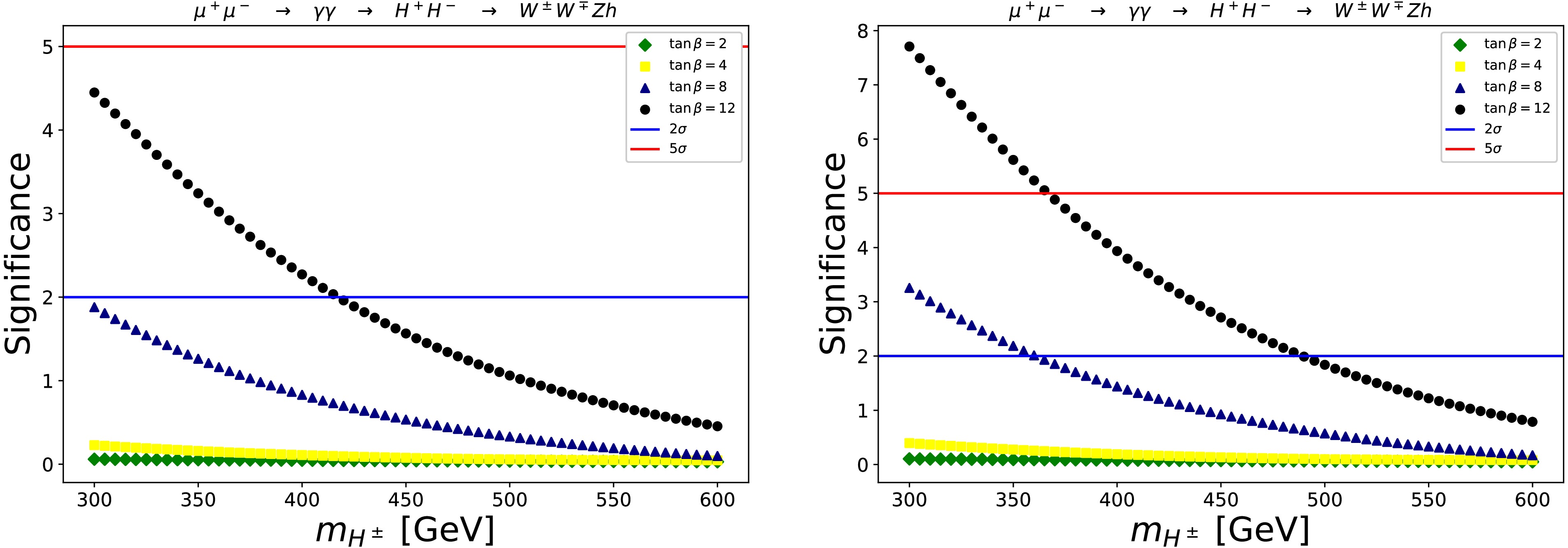
Figure 7. (color online) The corresponding signal significances taking into account the SM backgrounds are presented at
$ {\cal{L}}=1000 $ fb–1 in the left panel and at$ {\cal{L}}=3000 $ fb–1 in the right panel.
Figure D2. Feynman diagrams for
$ \mu^+\mu^- \rightarrow H^{+}H^{-} $ generated with$ {\mathrm{FeynArts}}$ [61]. -
We now turn our attention to another process,
$ \mu^+\mu^- \rightarrow \gamma \gamma \rightarrow H^{+}H^{-} \rightarrow W^{\pm}W^{\mp}Zh $ . The total cross section is calculated by convoluting the partonic process$ \gamma \gamma \rightarrow H^{+}H^{-} \rightarrow W^{\pm}W^{\mp}Zh $ with the photon structure function as follows:$ \sigma(s) = \int_{\tfrac{2m_{H^\pm}} {\sqrt{s}}}^{x_{\text{max}}} {\rm d}z \, \left( 2z \int_{z^2/x_{\text{max}}}^{x_{\text{max}}} \frac{{\rm d}x}{x} \, f_{\gamma/\mu}(x) \, f_{\gamma/\mu} \left(z^2/x\right) \right) \, \hat{\sigma}(\hat{s} = z^2 s). $
(13) Here, the photon structure function
$ f_{\gamma/\mu}(x) $ is used, with x denoting the energy fraction of the photon emitted by the incoming lepton. The explicit formulas for$ f_{\gamma/\mu}(x) $ are given in [67] with the appropriate of$ m_{\ell}=m_{\mu} $ as in [68] for example. In the master formulas, we adopt$ x_{\rm max} = 0.83 $ as in [69]. All tree-level Feynman diagrams for the process$ \gamma \gamma \to H^\pm H^\mp $ within the THDM are shown in Fig. D2. The partonic process$ \gamma \gamma \to H^+ H^- $ are generated by FeynArts/ FormCalc [61]. The SM background which is the process$ \gamma \gamma \to W^\pm W^\mp Z h $ , is calculated using the the$ {\mathrm{GRACE}}$ program [65]. To reduce the SM background, we apply cuts on the invariant masses of the final-state particles:$ |m_{Wh}-m_{H^\pm}| < 10 $ GeV and and$ |m_{WZ}-m_{H^\pm}| < 10 $ GeV. In Fig. 6, the numbers of events of the process$ \mu^+\mu^- \to \gamma\gamma \rightarrow H^{+}H^{-} \rightarrow W^{\pm}W^{\mp}Zh $ at an integrated luminosity of$ {\cal{L}}=3000\; \text{fb}^{-1} $ are shown in the left panel of Fig. 6. The signal significances considering the Standard Model backgrounds are presented at$ {\cal{L}}=500 $ fb–1 in the right panel of Fig. 6, while the significances are presented at$ {\cal{L}}=1000 $ fb–1 on the left panel and at$ {\cal{L}}=5000 $ fb–1 on the right panel of Fig. 7. We observe that the events become significant when the charged Higgs masses are in the low-mass region and$ t_{\beta} = 8, 12 $ , whereas they are small and can be ignored in other regions. For charged Higgs masses in the low-mass region and$ t_{\beta} = 12 $ , the significance can exceed$ 5\sigma $ . In other cases, the significances are negligible.
Figure 6. (color online) The signal events of the process
$ \mu^+\mu^- \to \gamma\gamma \rightarrow H^{+}H^{-} \rightarrow W^{\pm}W^{\mp}Zh $ at an integrated luminosity of$ {\cal{L}}=3000\; \text{fb}^{-1} $ are shown in the left panel. The corresponding signal significance taking into account the SM backgrounds is presented at$ {\cal{L}}=500\; \text{fb}^{-1} $ in the right panel.
Figure 7. (color online) The corresponding signal significances taking into account the SM backgrounds are presented at
$ {\cal{L}}=1000 $ fb–1 in the left panel and at$ {\cal{L}}=3000 $ fb–1 in the right panel.
Figure D2. Feynman diagrams for
$ \mu^+\mu^- \rightarrow H^{+}H^{-} $ generated with$ {\mathrm{FeynArts}}$ [61]. -
We now turn our attention to another process,
$ \mu^+\mu^- \rightarrow \gamma \gamma \rightarrow H^{+}H^{-} \rightarrow W^{\pm}W^{\mp}Zh $ . The total cross section is calculated by convoluting the partonic process$ \gamma \gamma \rightarrow H^{+}H^{-} \rightarrow W^{\pm}W^{\mp}Zh $ with the photon structure function, as follows:$ \sigma(s) = \int_{\tfrac{2m_{H^\pm}} {\sqrt{s}}}^{x_{\text{max}}} dz \, \left( 2z \int_{z^2/x_{\text{max}}}^{x_{\text{max}}} \frac{dx}{x} \, f_{\gamma/\mu}(x) \, f_{\gamma/\mu} \left(z^2/x\right) \right) \, \hat{\sigma}(\hat{s} = z^2 s). $
(13) Here, the photon structure function
$ f_{\gamma/\mu}(x) $ is used, with x denoting the energy fraction of the photon emitted by the incoming lepton. The explicit formulas for$ f_{\gamma/\mu}(x) $ are given in [65] with applying$ m_{\ell}=m_{\mu} $ appropriately, as used in [66] for example. In the master formulas, we adopt$ x_{\rm max} = 0.83 $ as in [67]. All tree-level Feynman diagrams for the process$ \gamma \gamma \to H^\pm H^\mp $ within the THDM are shown in Fig. D2. The partonic process$ \gamma \gamma \to H^+ H^- $ are generated by FeynArts/FormCalc [68]. The SM background which is the process$ \gamma \gamma \to W^\pm W^\mp Z h $ , is calculated using the$ {\mathrm{GRACE}}$ program [64]. To reduce the SM background, we apply cuts on the invariant masses of the final-state particles:$ |m_{Wh}-m_{H^\pm}| < 10 $ GeV and$ |m_{WZ}-m_{H^\pm}| < 10 $ GeV. In Figs. 6, the numbers of events of the process$ \mu^+\mu^- \to \gamma\gamma \rightarrow H^{+}H^{-} \rightarrow W^{\pm}W^{\mp}Zh $ at an integrated luminosity of$ {\cal{L}}=3000\; \text{fb}^{-1} $ are shown in the left panel of Fig. 6. The signal significances, taking into account the Standard Model backgrounds, are presented at$ {\cal{L}}=500 $ fb-1 in the right panel of Fig. 6. While the significances are presented at$ {\cal{L}}=1000 $ fb-1 on the left panel and at$ {\cal{L}}=5000 $ fb-1 on the right panel of Fig. 7. We observe that the events become significant when the charged Higgs masses are in the low-mass region and$ t_{\beta} = 8, 12 $ , whereas they are small and can be ignored in other regions. For charged Higgs masses in the low-mass region and$ t_{\beta} = 12 $ , the significance can exceed$ 5\sigma $ . In other cases, the significances are negligible.
Figure 6. (color online) The signal events of the process
$ \mu^+\mu^- \to \gamma\gamma \rightarrow H^{+}H^{-} \rightarrow W^{\pm}W^{\mp}Zh $ at an integrated luminosity of$ {\cal{L}}=3000\; \text{fb}^{-1} $ are shown in the left panel. The corresponding signal significance taking into account the SM backgrounds is presented at$ {\cal{L}}=500\; \text{fb}^{-1} $ in the right panel.
Figure 7. (color online) The corresponding signal significances taking into account the SM backgrounds are presented at
$ {\cal{L}}=1000 $ fb-1 in the left panel and at$ {\cal{L}}=3000 $ fb-1 in the right panel.
Figure D2. Feynman diagrams for
$ \mu^+\mu^- \rightarrow H^{+}H^{-} $ are generated by$ {\mathrm{FeynArts}}$ [68]. -
We now turn our attention to another process,
$ \mu^+\mu^- \rightarrow \gamma \gamma \rightarrow H^{+}H^{-} \rightarrow W^{\pm}W^{\mp}Zh $ . The total cross section is calculated by convoluting the partonic process$ \gamma \gamma \rightarrow H^{+}H^{-} \rightarrow W^{\pm}W^{\mp}Zh $ with the photon structure function as follows:$ \sigma(s) = \int_{\tfrac{2m_{H^\pm}} {\sqrt{s}}}^{x_{\text{max}}} {\rm d}z \, \left( 2z \int_{z^2/x_{\text{max}}}^{x_{\text{max}}} \frac{{\rm d}x}{x} \, f_{\gamma/\mu}(x) \, f_{\gamma/\mu} \left(z^2/x\right) \right) \, \hat{\sigma}(\hat{s} = z^2 s). $
(13) Here, the photon structure function
$ f_{\gamma/\mu}(x) $ is used, with x denoting the energy fraction of the photon emitted by the incoming lepton. The explicit formulas for$ f_{\gamma/\mu}(x) $ are given in [67] with the appropriate of$ m_{\ell}=m_{\mu} $ as in [68] for example. In the master formulas, we adopt$ x_{\rm max} = 0.83 $ as in [69]. All tree-level Feynman diagrams for the process$ \gamma \gamma \to H^\pm H^\mp $ within the THDM are shown in Fig. D2. The partonic process$ \gamma \gamma \to H^+ H^- $ are generated by FeynArts/ FormCalc [61]. The SM background which is the process$ \gamma \gamma \to W^\pm W^\mp Z h $ , is calculated using the the$ {\mathrm{GRACE}}$ program [65]. To reduce the SM background, we apply cuts on the invariant masses of the final-state particles:$ |m_{Wh}-m_{H^\pm}| < 10 $ GeV and and$ |m_{WZ}-m_{H^\pm}| < 10 $ GeV. In Fig. 6, the numbers of events of the process$ \mu^+\mu^- \to \gamma\gamma \rightarrow H^{+}H^{-} \rightarrow W^{\pm}W^{\mp}Zh $ at an integrated luminosity of$ {\cal{L}}=3000\; \text{fb}^{-1} $ are shown in the left panel of Fig. 6. The signal significances considering the Standard Model backgrounds are presented at$ {\cal{L}}=500 $ fb–1 in the right panel of Fig. 6, while the significances are presented at$ {\cal{L}}=1000 $ fb–1 on the left panel and at$ {\cal{L}}=5000 $ fb–1 on the right panel of Fig. 7. We observe that the events become significant when the charged Higgs masses are in the low-mass region and$ t_{\beta} = 8, 12 $ , whereas they are small and can be ignored in other regions. For charged Higgs masses in the low-mass region and$ t_{\beta} = 12 $ , the significance can exceed$ 5\sigma $ . In other cases, the significances are negligible.
Figure 6. (color online) The signal events of the process
$ \mu^+\mu^- \to \gamma\gamma \rightarrow H^{+}H^{-} \rightarrow W^{\pm}W^{\mp}Zh $ at an integrated luminosity of$ {\cal{L}}=3000\; \text{fb}^{-1} $ are shown in the left panel. The corresponding signal significance taking into account the SM backgrounds is presented at$ {\cal{L}}=500\; \text{fb}^{-1} $ in the right panel.
Figure 7. (color online) The corresponding signal significances taking into account the SM backgrounds are presented at
$ {\cal{L}}=1000 $ fb–1 in the left panel and at$ {\cal{L}}=3000 $ fb–1 in the right panel.
Figure D2. Feynman diagrams for
$ \mu^+\mu^- \rightarrow H^{+}H^{-} $ generated with$ {\mathrm{FeynArts}}$ [61]. -
In this article, we have calculated one-loop contributions for the decay process
$ H^{\pm} \rightarrow W^{\pm} Z $ in the Two-Higgs-Doublet Model and examined the posibility searches for charged Higgs pair production at future muon–TeV colliders. The computations have performed in the$ {\cal{R}}_{\xi} $ gauge, where the analytical results are verified through self-consistency tests such as ξ-independence, ultraviolet finiteness, and renormalization-scale stability of the process amplitude. The numerical results demonstrate good stability. We have revisited the parameter scan for the Type-X THDM in the phenomenological results. Based on the updated viable parameter space, we have analyzed charged Higgs pair production at future muon–TeV colliders by considering the processes$ \mu^+\mu^- \rightarrow H^+H^- \rightarrow W^{\pm}W^{\mp}Zh $ and$ \mu^+\mu^- \rightarrow \gamma\gamma \rightarrow H^+H^- \rightarrow W^{\pm}W^{\mp}Zh $ . The corresponding signal events and statistical significances are simulated with respect to the relevant SM backgrounds. Our findings show that the signal significance can exceed$ 5\sigma $ at several benchmark points within the viable parameter space of the Type-X THDM. -
In this article, we have calculated one-loop contributions for the decay process
$ H^{\pm} \rightarrow W^{\pm} Z $ in the Two-Higgs-Doublet Model and examined the posibility searches for charged Higgs pair production at future muon–TeV colliders. The computations have been performed in the$ {\cal{R}}_{\xi} $ gauge, and the analytical results were verified through self-consistency tests such as ξ-independence, ultraviolet finiteness, and renormalization-scale stability of the process amplitude. The numerical results demonstrate good stability. We have revisited the parameter scan for the Type-X THDM in the phenomenological results. Based on the updated viable parameter space, we have analyzed charged Higgs pair production at future muon–TeV colliders by considering the processes$ \mu^+\mu^- \rightarrow H^+H^- \rightarrow W^{\pm}W^{\mp}Zh $ and$ \mu^+\mu^- \rightarrow \gamma\gamma \rightarrow H^+H^- \rightarrow W^{\pm}W^{\mp}Zh $ . The corresponding signal events and statistical significances were simulated with respect to the relevant SM backgrounds. Our findings show that the signal significance can exceed$ 5\sigma $ at several benchmark points within the viable parameter space of the Type-X THDM. -
The conventions for one-loop one-, two-, and three-point tensor integrals with rank P, following Refs. [70, 59, 71], are given by
$ \{A; B; C\}^{\mu_1\mu_2\cdots \mu_P}= (\mu^2)^{2-d/2} \int \frac{d^dk}{(2\pi)^d} \dfrac{k^{\mu_1}k^{\mu_2} \cdots k^{\mu_P}}{\{D_1; D_1 D_2; D_1 D_2 D_3\}}. $
(A1) Here,
$ D_j^{-1} $ ($ j = 1, \cdots, 3 $ ) are the Feynman propagators defined as$ D_j = (k + q_j)^2 - m_j^2 + i\rho, $
(A2) where
$ q_j = \sum\limits_{i=1}^j p_i $ ,$ p_i $ are the external momenta, and$ m_j $ are the internal masses in the loops. Dimensional regularization for one-loop integrals is performed in a space–time dimension$ d = 4 - 2\varepsilon $ (the UV-divergent part is isolated as$ C_{UV} = 1/\varepsilon + \log(4\pi) - \Gamma_E $ ,$ \Gamma_E $ is the Euler–Mascheroni constant). In the above expressions, the parameter$ \mu^2 $ serves as the renormalization scale. Explicit reduction formulas for one-, two-, and three-point tensor integrals up to rank$ P = 3 $ are given in Ref. [70].$ A^{\mu} = 0, $
(A3) $ A^{\mu\nu} = g^{\mu\nu} A_{00}, $
(A4) $ A^{\mu\nu\rho} = 0, $
(A5) $ B^{\mu} = q^{\mu} B_1, $
(A6) $ B^{\mu\nu} = g^{\mu\nu} B_{00} + q^{\mu}q^{\nu} B_{11}, $
(A7) $ B^{\mu\nu\rho} = \{g, q\}^{\mu\nu\rho} B_{001} + q^{\mu}q^{\nu}q^{\rho} B_{111}, $
(A8) $ C^{\mu} = q_1^{\mu} C_1 + q_2^{\mu} C_2 = \sum\limits_{i=1}^2q_i^{\mu} C_i, $
(A9) $ C^{\mu\nu} = g^{\mu\nu} C_{00} + \sum\limits_{i,j=1}^2q_i^{\mu}q_j^{\nu} C_{ij}, $
(A10) $ C^{\mu\nu\rho} = \sum\limits_{i=1}^2 \{g,q_i\}^{\mu\nu\rho} C_{00i}+ \sum\limits_{i,j,k=1}^2 q^{\mu}_i q^{\nu}_j q^{\rho}_k C_{ijk}. $
(A11) The detailed expressions for these form factors in the general
$ R_{\xi} $ gauge are given in the following paragraphs. In the analytical expressions below, we have used the notations as follows:$ A_{ij\cdots}(P) = A_{ij\cdots}(M_P^2), $
(A12) $ B_{ij\cdots}(p^2; P_1, P_2) = B_{ij\cdots}(p^2; M_{P_1}^2,M_{P_2}^2 ), $
(A13) $\begin{aligned}[b]& C_{ij\cdots}(p_1^2, p_2^2, p_3^2; P_1, P_2,P_3) \\=\;& C_{ij\cdots}(p_1^2, p_2^2, p_3^2; M_{P_1}^2, M_{P_2}^2, M_{P_3}^2). \end{aligned} $
(A14) The analytic formulas for all form factors are expressed in terms of PV-functions, using the adopted shorthand notations as presented in the following paragraphs.
${\underline{Form\ factors\ {\cal{T}}^{B}_{i, \text{Trig}} } }$ :The form factor
$ {\cal{T}}^{B}_{i,\text{Trig}} $ ($ i = 1,2,3 $ ) is expressed in terms of the main contributions involving scalar Higgs bosons$ \phi \equiv h, H $ , together with charged particles such as$ H^\pm, W^\pm, G^\pm $ , and neutral particles including$ A, Z, G^0 $ circulating in the loop.$ {\cal{T}}^{B}_{i, \text{Trig}} = \sum \limits_{\phi = h, H} \Big( {\cal{T}}^{B, \phi-A}_{i, \text{Trig}} + {\cal{T}}^{B, \phi-H^\pm}_{i, \text{Trig}} + {\cal{T}}^{B, \phi-W^\pm}_{i, \text{Trig}} + {\cal{T}}^{B, \phi-Z}_{i, \text{Trig}} + {\cal{T}}^{B, \phi-W^\pm Z}_{i, \text{Trig}} \Big). $
(A15) Each contribution of
$ {\cal{T}}^{B}_{1, \text{Trig}} $ and$ {\cal{T}}^{B}_{2, \text{Trig}} $ is calculated from the corresponding Figs. A1, A2, A3, A4 and A5, respectively. Whereas, the form factor$ {\cal{T}}^{B}_{3, \text{Trig}} $ has no contribution in one-loop boson-exchanging diagrams. In the Fig. A1, the contribution in first for exchanging of ϕ and the pseudo-scalar Higgs A are reading as follows: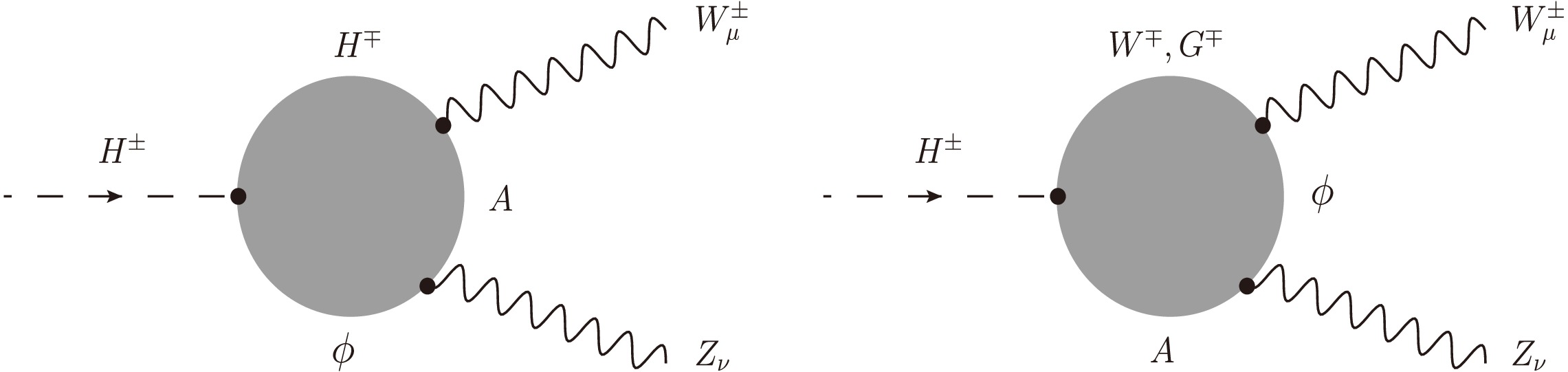
Figure A1. One-loop triangle Feynman diagrams with
$\phi = h, H, A$ , together with$H^\pm$ or$W^\pm$ propagating in the loop.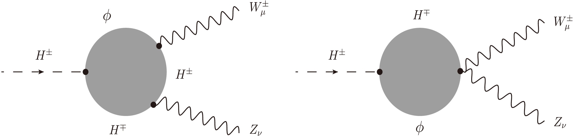
Figure A2. One-loop triangle Feynman diagrams with
$\phi = h, H$ and$H^\pm$ in the loop.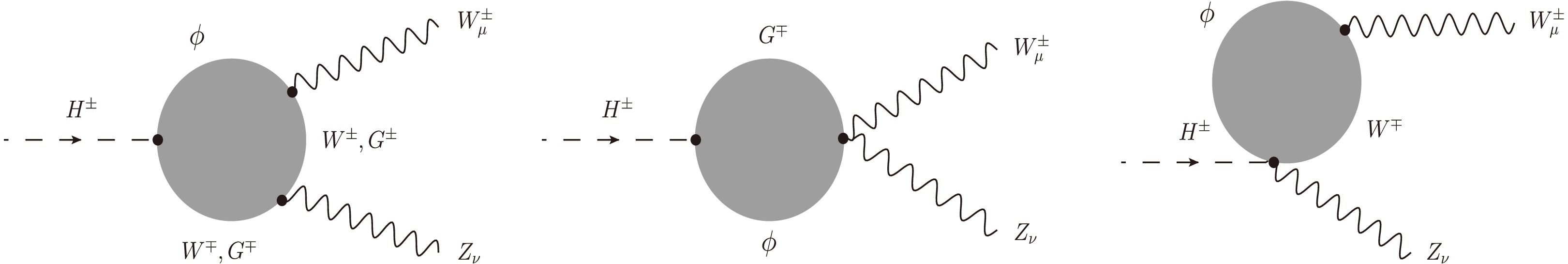
Figure A3. One-loop triangle diagrams with
$\phi = h, H$ and$W^\pm$ in the loop.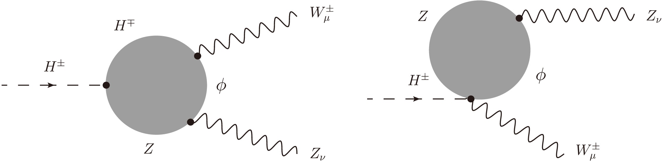
Figure A4. One-loop triangle diagrams with
$\phi = h, H$ and Z as internal lines in the loop.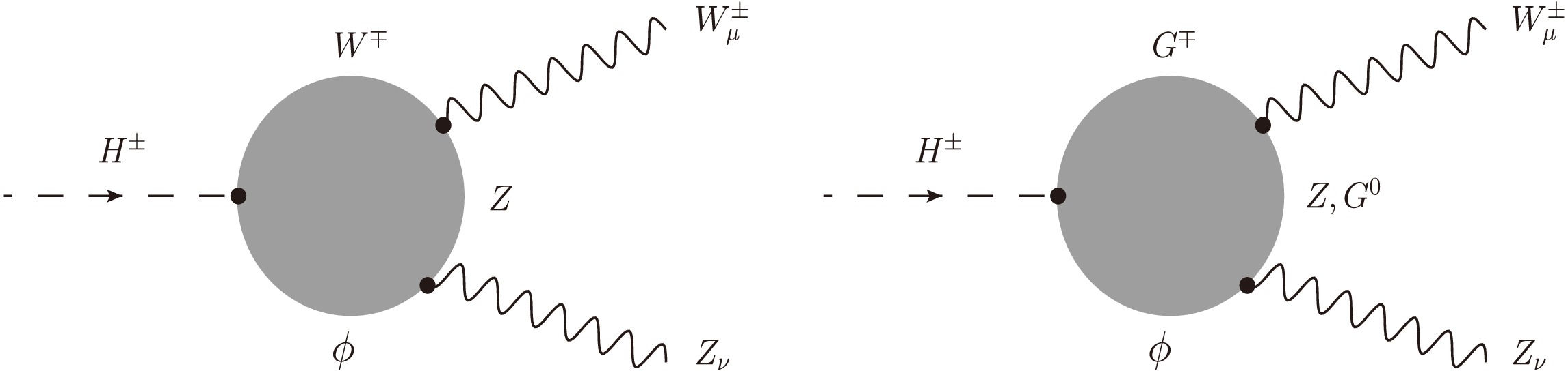
Figure A5. One-loop triangle Feynman diagrams with $\phi = h, H$ exchanging in association with $W^\pm$ and $Z$ contributions in the loop.
$ \begin{aligned}[b] \dfrac{ {\cal{T}}^{B, \phi-A}_{1, \text{Trig}} }{ g_{A H^- W^+} \cdot g_{\phi A Z} } =\;& - \dfrac{ g_{\phi W^\pm W^\mp} }{ 8\pi^2 \cdot m_W^2 } \big[ \big( m_{A}^2 +m_{H^\pm}^2 -\xi_{W} m_{W}^2 \big) C_{00} + 2 m_{H^\pm}^2 C_{002} + \big( m_{H^\pm}^2 -m_{W}^2 +m_{Z}^2 \big) C_{001} \big] (Z,W,H^\pm; A,\phi,\xi_W W ) \\& + \dfrac{ g_{\phi W^\pm W^\mp} }{ 8\pi^2 \cdot m_W^2 } \big[ 2 m_{H^\pm}^2 C_{00} + \big( m_{H^\pm}^2 -m_{W}^2 +m_{Z}^2 \big) C_{001} + 2 m_{H^\pm}^2 C_{002} \big] (Z,W,H^\pm;A,\phi,W) \\& - \dfrac{ g_{\phi H^\pm H^\mp} }{ 4\pi^2 } C_{00}(Z,H^\pm,W;A, \phi,H^\pm), \end{aligned} $
(A16) $\begin{aligned}[b] \dfrac{ {\cal{T}}^{B, \phi-A}_{2, \text{Trig}} }{ g_{A H^- W^+} \cdot g_{\phi A Z} } =\;& \dfrac{ g_{\phi W^\pm W^\mp} }{8\pi^2 \cdot m_W^2} \Big[ 2 \big( C_{00} + C_{001} \big) + \big( m_{H^\pm}^2 -m_{W}^2 +m_{Z}^2 \big) C_{112} + \big( 3 m_{H^\pm}^2 -m_{W}^2 +m_{Z}^2 \big) \big( C_{12} + C_{122} \big) + 4 \big( m_{H^\pm}^2 C_{22} + C_{002} \big) \\ & + 2 \big( m_{H^\pm}^2 -m_{W}^2 \big) C_{2} + 2 m_{H^\pm}^2 C_{222} \Big] (Z,W,H^\pm; A,\phi,W) + \dfrac{ g_{\phi W^\pm W^\mp} }{8\pi^2 \cdot m_W^2} \Big[ \big( m_{W}^2 -m_{Z}^2 -3 m_{H^\pm}^2 \big) C_{122}\\ & - 2 \big( C_{00} + C_{001} + 2 C_{002} \big) - \big( m_{A}^2 +m_{H^\pm}^2 -\xi_{W} m_{W}^2 \big) C_{2} - \big( m_{H^\pm}^2 -m_{W}^2 +m_{Z}^2 \big) C_{112}\\ & - \Big( m_{A}^2 +2 m_{H^\pm}^2 - \big( \xi_{W}+1 \big) m_{W}^2 + m_{Z}^2 \Big) C_{12} - 2 m_{H^\pm}^2 C_{222} \\ &- \big( m_{A}^2 +3 m_{H^\pm}^2 -\xi_{W} m_{W}^2 \big) C_{22} \Big](Z,W, H^\pm; A, \phi, \xi_W W) + \dfrac{ g_{\phi H^\pm H^\mp} }{4\pi^2} C_{12} (Z,H^\pm,W; A, \phi, H^\pm), \end{aligned} $
(A17) $ \dfrac{ {\cal{T}}^{B, \phi-A}_{3, \text{Trig}} }{ g_{A H^- W^+} \cdot g_{\phi A Z} } = 0. $
(A18) Following Fig. A2, the one-loop contributions from the exchange of ϕ and the charged Higgs
$ H^\pm $ are expressed as follows:$ \begin{aligned}[b]& \dfrac{ {\cal{T}}^{B, \phi-H^\pm}_{1, \text{Trig}} }{ 16\pi^2 \cdot g_{\phi H^\pm H^\mp} } = g_{\phi H^-W^+Z} \cdot B_{0}(H^\pm;\phi,H^\pm)\\&\quad - 4 \, g_{\phi H^- W^+} \cdot g_{Z H^\pm H^\mp} \, C_{00}(W,Z,H^\pm;\phi,H^\pm, H^\pm), \end{aligned}$
(A19) $\begin{aligned}[b] \dfrac{ {\cal{T}}^{B, \phi-H^\pm}_{2, \text{Trig}} }{ 16\pi^2 \cdot g_{\phi H^\pm H^\mp} } =\;& -4 g_{\phi H^- W^+} \cdot g_{Z H^\pm H^\mp} \big( C_{2} + C_{12} + C_{22} \big)\\&\times (W,Z, H^\pm; \phi,H^\pm, H^\pm), \end{aligned} $
(A20) $ \dfrac{ {\cal{T}}^{B, \phi-H^\pm}_{3, \text{Trig}} }{ 16\pi^2 \cdot g_{\phi H^\pm H^\mp} } = 0. $
(A21) From Fig. A3, we obtain the form factors involving the neutral scalar Higgs boson ϕ in association with the vector boson
$ W^\pm $ and the Goldstone bosons$ G^\pm $ in the loop. The factor is given by$ \begin{aligned}[b] \dfrac{ {\cal{T}}^{B, \phi-W^\pm}_{1, \text{Trig}} } { g_{\phi W^\pm W^\mp} } = \;&\dfrac{ g_{\phi H^- W^+} \cdot g_{Z W^\pm W^\mp} }{32\pi^2 \cdot m_{W}^4} \Big\{ 2 m_{W}^2 \Big[ A_{0}(W) - A_{0}(\xi_W W) \Big] + \Big[ 2 m_{W}^2 \big( m_{H^\pm}^2 -m_{\phi}^2 +m_{Z}^2 -m_{W}^2 \big) B_{0} - 2 m_{Z}^2 B_{00} \Big] (Z; W,\xi_{W} W) \\& + \Big[ 2 m_{W}^2 \big( m_{\phi}^2 -m_{H^\pm}^2 -m_{Z}^2 \big) B_{0} + 2 \big( m_{Z}^2 -m_{W}^2 \big) B_{00} \Big](Z; W, W) + 2 m_{W}^2 B_{00}(Z;\xi_{W} W, \xi_{W} W ) \\ &- s_{W}^2 m_{Z}^2 \big( m_{\phi}^2 -m_{H^\pm}^2 \big) B_{0} (H^\pm; \phi, \xi_W W) + 2 m_{W}^2 \Big[ \big( m_{H^\pm}^2 - m_{\phi}^2 \big) \big( m_{H^\pm}^2 +m_{W}^2 -m_{Z}^2 \big) C_{2} + 2 m_{W}^2 \big( m_{H^\pm}^2 -m_{\phi}^2 \big) C_{1} \\ & - m_{\phi}^2 \big( m_{\phi}^2 -m_{H^\pm}^2 \big) C_{0} \Big] (W,Z, H^\pm;\phi,W, \xi_W W) + 2 m_{W}^2 \Big[ \big( m_{W}^2 -m_{H^\pm}^2 -m_{\phi}^2 \big) C_{00} - \big( m_{H^\pm}^2 +m_{W}^2 -m_{Z}^2 \big) C_{002} \\ & - 2 m_{H^\pm}^2 C_{001} \Big](H^\pm, Z, W; \phi,W, \xi_W W) \Big\} + \dfrac{ g_{\phi H^- W^+} \cdot g_{Z W^\pm W^\mp} }{32\pi^2 \cdot m_{W}^4} \Big\{ 2 m_{W}^2 \Big[ \big( m_{H^\pm}^2 +m_{W}^2 -m_{Z}^2 \big) C_{001} + 2 m_{H^\pm}^2 C_{002} \Big] \\ & + 2 m_{W}^2 \Big[ m_{\phi}^4 - m_{\phi}^2 \big( m_{H^\pm}^2 +m_{Z}^2 \big) - \big( m_{H^\pm}^2 -m_{W}^2 \big) \big( m_{W}^2 -m_{Z}^2 \big) \Big] C_{0} + 2 \Big[ m_{\phi}^2 \big( m_{Z}^2 -m_{W}^2 \big) - m_{Z}^2 \big( m_{H^\pm}^2 +m_{W}^2 \big) \\ &+ m_{W}^2 \big( 3 m_{H^\pm}^2 +m_{W}^2 \big) \Big] C_{00} + 2 m_{W}^4 \big( 2 m_{\phi}^2 -m_{H^\pm}^2 -m_{W}^2 -m_{Z}^2 \big) C_{1} + 2 m_{W}^2 \Big[ m_{\phi}^2 \big( m_{H^\pm}^2 +m_{W}^2 -m_{Z}^2 \big)\\ & + m_{H^\pm}^2 \big( m_{Z}^2 -m_{H^\pm}^2 \big) + m_{W}^2 \big( m_{Z}^2 -m_{W}^2 \big) \Big] C_{2} \Big\} (W,Z,H^\pm;\phi, W, W) \\& - \dfrac{ g_{\phi H^- W^+ Z} }{16\pi^2 \cdot m_{W}^2} \Big[ \big( m_{W}^2 B_{0} - B_{00} \big) (W;\phi,W) + B_{00} (W,\phi,\xi_W W) \Big], \end{aligned} $
(A22) $ \begin{aligned}[b] \dfrac{ {\cal{T}}^{B, \phi-W^\pm}_{2, \text{Trig}} } { g_{\phi W^\pm W^\mp} } =\;& - \dfrac{ g_{\phi H^- W^+} \cdot g_{Z W^\pm W^\mp} }{8\pi^2 \cdot m_{W}^2} \Big\{ \big( B_{0} + B_{1} \big) (Z;W,\xi_{W} W ) + B_{1}(Z;W, W) \Big\} - \dfrac{ g_{\phi H^- W^+} \cdot g_{Z W^\pm W^\mp} }{16\pi^2 \cdot m_{W}^4} \times \Big\{ 4 m_{W}^4 C_{1} \\&+ \Big[ m_{W}^2 \big( 3 m_{\phi}^2 -m_{H^\pm}^2 +m_{W}^2 \big) - m_{Z}^2 \big( m_{\phi}^2 -m_{H^\pm}^2 +m_{W}^2 \big) \Big] C_{2} + \Big[ m_{\phi}^2 \big( m_{W}^2 -m_{Z}^2 \big) + m_{H^\pm}^2 \big( m_{Z}^2 -2 m_{W}^2 \big) \Big] C_{12}\\& + 2 m_{W}^2 \big( C_{00} - C_{001} - 2 C_{002} \big) + \big( m_{W}^2-m_{Z}^2 \big) \big( m_{\phi}^2 -m_{H^\pm}^2 -m_{W}^2 \big) C_{22} - m_{W}^2 \big( m_{H^\pm}^2 +m_{W}^2 -m_{Z}^2 \big) C_{112} \\ & + m_{W}^2 \big( m_{Z}^2 -m_{W}^2 -3 m_{H^\pm}^2 \big) C_{122} - 2 m_{H^\pm}^2 m_{W}^2 C_{222} \Big\} (W,Z,H^\pm;\phi,W,W ) - \dfrac{ g_{\phi H^- W^+} \cdot g_{Z W^\pm W^\mp} }{16\pi^2 \cdot m_{W}^4} \\& \times \Big\{ m_{W}^2 \big( m_{W}^2 -m_{\phi}^2 -m_{H^\pm}^2 \big) C_{1} + m_{W}^2 \big( m_{\phi}^2 -m_{H^\pm}^2 -m_{W}^2 \big) C_{11} + m_{W}^2 \big( m_{\phi}^2 -2 m_{W}^2 +m_{Z}^2 \big) C_{12} \\ &- 2 m_{W}^2 \big( C_{00} - C_{002} - 2 C_{001} \big) + m_{W}^2 \big( m_{W}^2 -m_{Z}^2 +3 m_{H^\pm}^2 \big) C_{112} + m_{W}^2 \big( m_{H^\pm}^2 +m_{W}^2 -m_{Z}^2 \big) C_{122} \\ & + 2 m_{H^\pm}^2 m_{W}^2 C_{111} \Big\} (H^\pm,Z, W; \phi, W, \xi_{W} W), \end{aligned}$
(A23) $ \dfrac{ {\cal{T}}^{B, \phi-W^\pm}_{3, \text{Trig}} }{ g_{\phi W^\pm W^\mp} } = 0. $
(A24) In Fig. A4, the corresponding one-loop form factors, with both Higgs bosons ϕ and the vector boson Z exchanged in the loop, are given as follows:
$\begin{aligned}[b] \dfrac{ {\cal{T}}^{B, \phi-Z}_{1, \text{Trig}} } { g_{\phi ZZ} } = \;& - \dfrac{ g_{\phi H^- W^+ Z} }{ 16\pi^2 \cdot m_{Z}^2} \Big[ \big( m_{Z}^2 B_{0} - B_{00} \big) (Z;\phi,Z)\\ & + B_{00} (Z;\phi,\xi_Z Z) \Big]- \dfrac{ g_{\phi H^- W^+} \cdot g_{Z H^\pm H^\mp} }{ 8\pi^2 \cdot m_{Z}^2} \\& \times \Big[ B_{00} (Z; \phi,Z) - B_{00} (Z;\phi,\xi_Z Z) \\& - m_{Z}^2 C_{00} (W,H^\pm,Z;\phi,H^\pm,Z) \Big], \end{aligned} $
(A25) $\begin{aligned}[b] \dfrac{ {\cal{T}}^{B, \phi-Z}_{2, \text{Trig}} } { g_{\phi ZZ} } =\;&- \dfrac{ g_{\phi H^- W^+} \cdot g_{Z H^\pm H^\mp} }{16\pi^2} \big( 4 C_{2} + 2 C_{12} \big)\\& \times (W,H^\pm,Z;\phi,H^\pm,Z), \end{aligned} $
(A26) $ \dfrac{ {\cal{T}}^{B, \phi-Z}_{3, \text{Trig}} } { g_{\phi ZZ} } = 0. $
(A27) In Fig. A5, the form factors corresponding to the neutral scalar Higgs ϕ, accompanied by both the vector bosons
$ W^\pm $ and Z and the Goldstone bosons$ G^\pm $ and$ G^0 $ in the loop, are represented as follows:$ \begin{aligned}[b] \dfrac{ {\cal{T}}^{B, \phi-W^\pm Z}_{1, \text{Trig}} } { g_{\phi ZZ} } = \dfrac{ g_{\phi H^- W^+} \cdot g_{Z W^\pm W^\mp} }{16\pi^2} \xi_{W} B_{0} (Z; \phi,Z) + \dfrac{ g_{\phi H^- W^+} \cdot g_{Z W^\pm W^\mp} }{16\pi^2 \cdot m_{W}^2 m_{Z}^2} \Big\{ \big[ c_{W}^2 m_{Z}^2 \big( m_{\phi}^2 -m_{H^\pm}^2 \big) \end{aligned} $
$ \begin{aligned}[b] &+ m_{W}^2 \big( 2 m_{H^\pm}^2 - \xi_{W} m_{W}^2 \big) \big] C_{00} + m_{W}^2 \big[ \big( m_{H^\pm}^2 -m_{W}^2 +m_{Z}^2 \big) C_{002} + 2 m_{H^\pm}^2 C_{001} \big] \Big\} (H^\pm, W, Z; \phi,\xi_{W} W, \xi_{Z} Z ) \\& + \dfrac{ g_{\phi H^- W^+} \cdot g_{Z W^\pm W^\mp} }{16\pi^2 \cdot m_{W}^2 m_{Z}^2} \Bigg\{ m_{Z}^2 \Big[ m_{H^\pm}^2 \big[ m_{W}^2 \big( 2-3 \xi_{W} \big) + m_{Z}^2 \big( s_{W}^2-2 \big) + 2 m_{H^\pm}^2 \big] - m_{\phi}^2 m_{Z}^2 s_{W}^2 + \xi_{W} m_{W}^2 \big[ m_{W}^2 \big( \xi_{W}-1 \big) + m_{Z}^2 \big] \Big] C_{0} \\& - m_{Z}^2 \Big[ m_{H^\pm}^2 \big( 2 m_{W}^2 + 2 m_{Z}^2- 3 m_{H^\pm}^2 \big) + 2 \xi_{W} m_{W}^2 \big( m_{H^\pm}^2 - m_{W}^2 \big) + \big( m_{W}^2 -m_{Z}^2 \big)^2 \Big] C_{1} + \Big[ m_{Z}^2 \big( m_{\phi}^2 s_{W}^2 +2 m_{W}^2 -2 m_{Z}^2 \big) \\ & - m_{H^\pm}^2 \big[ 2 m_{W}^2 + m_{Z}^2 \big( s_{W}^2-4 \big) \big] + \xi_{W} m_{W}^2 \big( m_{W}^2 -m_{Z}^2 \big) \Big] C_{00} - m_{Z}^2 \Big[ m_{H^\pm}^2 \big( 2 m_{W}^2 + 2 m_{Z}^2 -3 m_{H^\pm}^2 \big) + \big( m_{W}^2 -m_{Z}^2 \big)^2 \Big] C_{12} \\ & + m_{Z}^2 \Big[ \xi_{W} m_{W}^2 \big( m_{Z}^2 -m_{W}^2 -3 m_{H^\pm}^2 \big) + 4 m_{H^\pm}^2 \big( m_{H^\pm}^2 +m_{W}^2 -m_{Z}^2 \big) \Big] C_{2} + \big( m_{Z}^2 -m_{W}^2 \big) \Big[ 2 m_{H^\pm}^2 C_{002} + \big( m_{H^\pm}^2 -m_{W}^2 +m_{Z}^2 \big) C_{001} \Big] \\& + m_{Z}^2 \Big[ \big( m_{H^\pm}^2 -m_{W}^2 +m_{Z}^2 \big) \big( m_{H^\pm}^2 -m_{W}^2 -m_{Z}^2 \big) C_{11} + 2 m_{H^\pm}^2 \big( m_{H^\pm}^2 +m_{W}^2 -m_{Z}^2 \big) C_{22} \Big] \Bigg\} (Z,W,H^\pm; \phi,Z, \xi_W W) \\& + \dfrac{ g_{\phi H^- W^+} \cdot g_{Z W^\pm W^\mp} }{16\pi^2 \cdot m_{W}^2} \Bigg\{ 2 \big( m_{H^\pm}^2 +m_{W}^2 -m_{Z}^2 \big) \Big[ \big( m_{W}^2 - m_{H^\pm}^2 \big) C_{0} - C_{00} \Big] + \Big[ m_{H^\pm}^2 \big( 2 m_{W}^2 + 2 m_{Z}^2 -3 m_{H^\pm}^2 \big) + \big( m_{W}^2 -m_{Z}^2 \big)^2 \Big] \big( C_{2} + C_{12} \big) \\ & + \big( m_{H^\pm}^2 -m_{W}^2 +m_{Z}^2 \big) \Big[ \big( m_{W}^2 +m_{Z}^2 -m_{H^\pm}^2 \big) C_{22} - C_{002} \Big] - 2 m_{H^\pm}^2 \Big[ \big( m_{H^\pm}^2 +m_{W}^2 -m_{Z}^2 \big) \big( 2 C_{1} + C_{11} \big) + \big( C_{00} + C_{001} \big) \Big] \Bigg\}\\&\times (H^\pm, W, Z; \phi, W, Z), \end{aligned} $
(A28) $ \begin{aligned}[b] \dfrac{ {\cal{T}}^{B, \phi-W^\pm Z}_{2, \text{Trig}} }{ g_{\phi ZZ} } = \;& \dfrac{ g_{\phi H^- W^+} \cdot g_{Z W^\pm W^\mp} }{16\pi^2 \cdot m_{W}^2 m_{Z}^2} \Bigg\{ \Big[ m_{Z}^2 c_{W}^2 \big( m_{\phi}^2 - m_{H^\pm}^2 \big) + m_{W}^2 \big( 2 m_{H^\pm}^2 - \xi_{W} m_{W}^2 \big) \Big] C_{1} + \Big[ m_{Z}^2 c_{W}^2 \big( m_{\phi}^2 - m_{H^\pm}^2 \big) + m_{W}^2 \big( 4 m_{H^\pm}^2 - \xi_{W} m_{W}^2 \big) \Big] C_{11} \\& + \Big[ m_{Z}^2 \big( c_{W}^2 m_{\phi}^2 + m_{W}^2 \big) - m_{H^\pm}^2 \big( c_{W}^2 m_{Z}^2 - 3 m_{W}^2 \big) - m_{W}^4 \big( \xi_{W} + 1 \big) \Big] C_{12} + 2m_{W}^2 m_{H^\pm}^2 C_{111} + m_{W}^2 \big( 3 m_{H^\pm}^2 -m_{W}^2 +m_{Z}^2 \big) C_{112} \\& + m_{W}^2 \big( m_{H^\pm}^2 -m_{W}^2 +m_{Z}^2 \big) C_{122} + 2 m_{W}^2 \big( C_{00} + 2 C_{001} + C_{002} \big) \Bigg\} (H^\pm, W, Z; \phi,\xi_{W} W,\xi_{Z} Z ) \\ & + \dfrac{ g_{\phi H^- W^+} \cdot g_{Z W^\pm W^\mp} }{16\pi^2 \cdot m_{W}^2 m_{Z}^2} \Bigg\{ \big( m_{Z}^2 -m_{W}^2 \big) \Big[ 2 C_{00} + 2 C_{001} + 4 C_{002} + 2 m_{H^\pm}^2 C_{222} + \big( m_{H^\pm}^2 -m_{W}^2 +m_{Z}^2 \big) C_{112} \\ &+ \big( 3 m_{H^\pm}^2 -m_{W}^2 +m_{Z}^2 \big) C_{122} \Big] + \Big[ m_{\phi}^2 m_{Z}^2 s_{W}^2 - m_{H^\pm}^2 \big( m_{W}^2 - m_{Z}^2 \big) + \xi_{W} m_{W}^2 \big( m_{W}^2 -m_{Z}^2 \big) \Big] C_{2} + \Big[ m_{\phi}^2 m_{Z}^2 s_{W}^2 - 3 m_{H^\pm}^2 \big( m_{W}^2 - m_{Z}^2 \big)\\ & + \xi_{W} m_{W}^2 \big( m_{W}^2 -m_{Z}^2 \big) \Big] C_{22} - \Big[ 3 m_{H^\pm}^2 m_{W}^2 - m_{Z}^2 \big( m_{\phi}^2 s_{W}^2 + m_{Z}^2 \big) + m_{H^\pm}^2 m_{Z}^2 \big( s_{W}^2-3 \big) - m_{W}^4 \big( \xi_{W}+1 \big) \\ &+ m_{W}^2 m_{Z}^2 \big( \xi_{W}+2 \big) \Big] C_{12} \Bigg\} (Z,W,H^\pm; \phi,Z,\xi_W W) + \dfrac{ g_{\phi H^- W^+} \cdot g_{Z W^\pm W^\mp} }{16\pi^2 \cdot m_{W}^2 } \Bigg\{ \big( m_{W}^2 -m_{Z}^2 -3 m_{H^\pm}^2 \big) \big( C_{12} + C_{112} \big) \\ & - \big( m_{H^\pm}^2 -m_{W}^2 +m_{Z}^2 \big) C_{122} + 2 m_{W}^2 \big( C_{1} + 2 C_{2} \big) - 2 m_{H^\pm}^2 \big( C_{1} + 2 C_{11} + C_{111} \big) - 2 \big( C_{00}\\ & + 2 C_{001} + C_{002} \big) \Bigg\} (H^\pm,W,Z; \phi,W, Z), \\ \dfrac{ {\cal{T}}^{B, \phi-W^\pm Z}_{3, \text{Trig}} } { g_{\phi ZZ} } =\;& 0. \end{aligned} $
(A29) ${\underline{Form\ factors \ {\cal{T}}^{B}_{i, \text{Self}}}} $ :Following Fig. A6, the form factors
$ {\cal{T}}^{B}_{i, \text{Self}} $ for$ i = 1, 2, 3 $ are decomposed into two contributions from one-point$ (1P) $ and two-point$ (2P) $ Feynman diagrams. These factors are expressed as follows: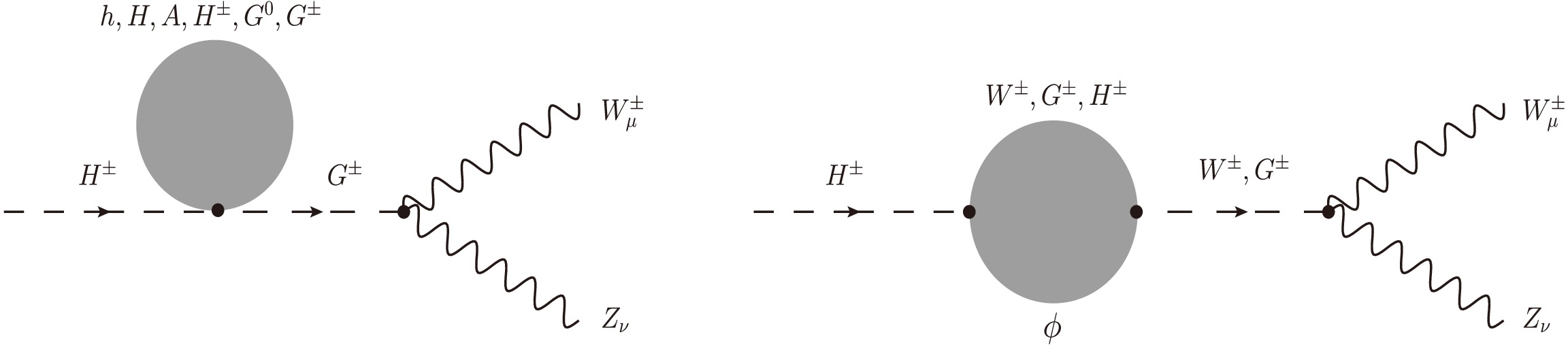
Figure A6. Self-energy Feynman diagram contributions to the external leg
$ H^\pm$ .$ {\cal{T}}^{B}_{i, \text{Self}} = {\cal{T}}^{B}_{i, \text{Self} - 1P} + \sum \limits_{\phi = h, H} \Big( {\cal{T}}^{B, \phi-H^\pm}_{i, \text{Self} - 2P} + {\cal{T}}^{B, \phi-W^\pm}_{i, \text{Self} - 2P} \Big) $
(A30) in which, these above form factors for
$ i = 1 $ are reading as follows$ \begin{aligned}[b] \dfrac{ {\cal{T}}^{B}_{1, \text{Self} - 1P} }{ g_{Z W^\pm W^\mp} } =\;& \dfrac{m_{W} s_{W}^2}{ 32\pi^2 \cdot c_{W}^2 \big(m_{H^\pm}^2 - \xi m_{W}^2\big) } \times \Bigg\{ g_{G^0 G^0 H^- G^+} \, A_0 (\xi_{Z} Z) + 2 g_{G^+ G^- H^- G^+} \, A_0 (\xi_{W} W) \\& + g_{A A H^- G^+} \, A_0 (A) + 2 g_{H^+ H^- H^- G^+} \, A_0 (H^\pm) + g_{h h \, H^- G^+} \, A_0 (h) + g_{H H \, H^- G^+} \, A_0 (H) \Bigg\}, \end{aligned}$
(A31) $ \begin{aligned}[b] \dfrac{ {\cal{T}}^{B, \phi-H^\pm}_{1, \text{Self} - 2P} }{ g_{Z W^\pm W^\mp} } =\;& - \dfrac{ g_{\phi H^- W^+} \cdot g_{\phi H^\pm H^\mp} }{ 16\pi^2 \cdot m_{W}^2 \big( m_{H^\pm}^2 - \xi_{W} m_{W}^2 \big)} \Bigg\{ 2 \xi_{W} m_{W}^2 \big( m_{W}^2 -m_{Z}^2 \big) B_{1}(H^\pm; \phi, H^\pm)\\ & + \Big[ m_{Z}^2 s_{W}^2 \big( m_{H^\pm}^2 - m_{\phi}^2 \big) + \xi_{W} m_{W}^2 \big( m_{W}^2 -m_{Z}^2 \big) \Big] B_{0}(H^\pm; \phi, H^\pm) \Bigg\}, \end{aligned} $
(A32) $ \begin{aligned}[b] \dfrac{{\cal{T}}^{B, \phi-W^\pm}_{1, \text{Self} - 2P} }{ g_{Z W^\pm W^\mp} } =\;& - \dfrac{ g_{\phi H^- W^+} \cdot g_{\phi W^\pm W^\mp} }{ 32\pi^2 \cdot m_{W}^4 \big( m_{H^\pm}^2 - \xi_{W} m_{W}^2 \big)} \times \Bigg\{ s_{W}^2 m_{Z}^2 \Big[ \big( m_{\phi}^2 -m_{H^\pm}^2 \big) A_{0} (W) - \big( m_{\phi}^2 -m_{H^\pm}^2 +\xi_{W} m_{W}^2 \big) A_{0} (\xi_{W} W) \Big] \\& + \big( m_{\phi}^2 -m_{H^\pm}^2 \big) \Big[ s_{W}^2 m_{H^\pm}^2 m_{Z}^2 + \xi_{W} m_{W}^2 \big( m_{W}^2 -m_{Z}^2 \big) \Big] B_{0} (H^\pm; \phi, \xi_{W} W) + 2 m_{W}^2 \Big[ \xi_{W} \big( m_{W}^2 -m_{Z}^2 \big) \big( m_{H^\pm}^2 +m_{W}^2 -m_{\phi}^2 \big) \\ & + s_{W}^2 m_{H^\pm}^2 m_{Z}^2 \Big] B_{1} (H^\pm; \phi,W) + s_{W}^2 m_{Z}^2 \Big[ \big( m_{\phi}^2 -m_{H^\pm}^2 \big)^2 - m_{W}^2 \big( m_{\phi}^2 +m_{H^\pm}^2 \big) \Big] B_{0} (H^\pm; \phi,W) \\& - 2 \xi_{W} m_{W}^2 \big( m_{W}^2 -m_{Z}^2 \big) \big( m_{\phi}^2 -m_{H^\pm}^2 +m_{W}^2 \big) B_{0} (H^\pm; \phi,W) \Bigg\}. \end{aligned} $
(A33) Other ones for
$ i = 2, 3 $ have no contribution, or$ {\cal{T}}^{B}_{i, \text{Self} - 1P} = {\cal{T}}^{B, \phi-H^\pm}_{i, \text{Self} - 2P} = {\cal{T}}^{B, \phi-W^\pm}_{i, \text{Self} - 2P} = 0. $
(A34) $ {\underline{Form\ factors \ {\cal{T}}^{B}_{i, \text{Tad}}}} $ :According to Fig. A7, the form factor
$ {\cal{T}}^{B}_{i, \text{Tad}} $ for$ i = 1, 2, 3 $ is expressed in terms of the scalar Higgs$ \phi \equiv h, H $ pole coupling with the bubble diagrams. In these loops, the neutral and pseudo-scalar Higgs particles$ h, H, A $ , the charged Higgs$ H^\pm $ , the vector bosons$ W^\pm $ and Z, the Goldstone bosons$ G^\pm $ and$ G^0 $ , and the corresponding ghost particles$ u_\pm $ and$ u_Z $ are all taken into account. As a result, the factor is given by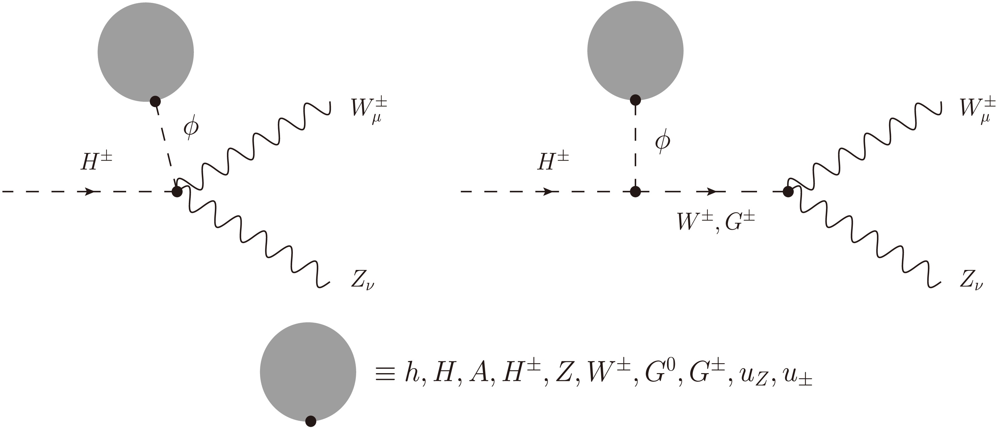
Figure A7. Tadpole Feynman diagram contributions with poles
$ \phi \equiv h, H$ .$ {\cal{T}}^{B}_{i, \text{Tad}} = \sum \limits_{\phi = h, H} {\cal{T}}^{B, \phi}_{i, \text{Tad}}. $
(A35) Where the form factors expressed as follows:
$ \begin{aligned}[b] {\cal{T}}^{B, \phi}_{1, \text{Tad}} = \;& - \dfrac{1}{ 64\pi^2 \cdot m_{\phi}^2 \big(m_{H^\pm}^2 - \xi_{W} m_{W}^2 \big) } \times \Big[ g_{\phi H^- W^+ Z} \, \big( m_{H^\pm}^2 - \xi_{W} m_{W}^2 \big) + \big( m_{\phi}^2 -m_{H^\pm}^2 \big) t_{W}^2\; g_{\phi H^- W^+} \cdot g_{Z W^\pm W^\mp} \\& + \xi_{W} \big( m_{Z}^2 -m_{W}^2 \big) g_{\phi H^- W^+} \cdot g_{Z W^\pm W^\mp} \Big] \times \Bigg\{ 4 m_{Z}^2 \, g_{\phi Z Z} + 8 m_{W}^2 \, g_{\phi W^\pm W^\mp} + 2 g_{\phi A A} \; A_{0} (A) + 2 g_{\phi h h} \; A_{0} (h) \\ & + 2 \; g_{\phi H H} \, A_{0} (H) + 4 g_{\phi H^\pm H^\mp} \, A_{0} (H^\pm) - 12 g_{\phi W^\pm W^\mp} A_{0} (W) - 6 g_{\phi Z Z} \, A_{0} (Z) - g_{\phi Z Z} \, \dfrac{m_{\phi}^2}{m_{Z}^2} \; A_{0} (\xi_{Z} Z) \\& - 2 \dfrac{m_{\phi}^2}{m_{W}^2} \, g_{\phi W^\pm W^\mp} \, A_{0} (\xi_{W} W) \Bigg\}, \end{aligned}$
(A36) $ {\cal{T}}^{B, \phi}_{2, \text{Tad}} = {\cal{T}}^{B, \phi}_{3, \text{Tad}} = 0. $
(A37) $ {\underline{Form\ factors \ {\cal{T}}^{F}_{i, \text{Trig}}}} $ :The form factors
$ {\cal{T}}^{F}_{i, \text{Trig}} $ , for$ i = 1, 2, 3 $ as depicted in the corresponding Fig. A8 are given by: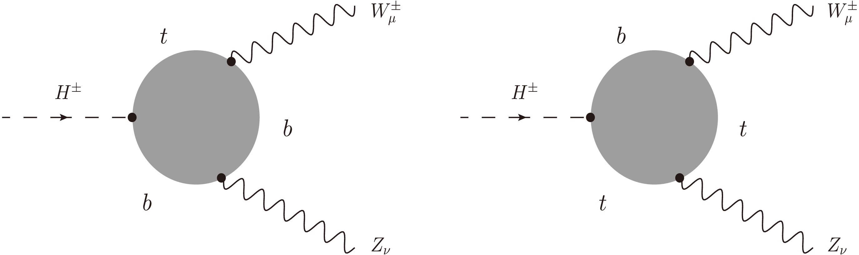
Figure A8. One-loop triangle Feynman diagrams with fermion loops.
$ \begin{aligned}[b] \dfrac{{\cal{T}}^{F}_{1, \text{Trig}} }{ g_{W^+ \bar{t} \, b} } =\;& \dfrac{ N^C_Q }{ 8\pi^2} \cdot \Bigg\{ g^{L}_{H^- t \bar{b}} \, m_{b}^2 \, \Big[ g^{L}_{Z t \bar{t}} \, B_{0} (Z; t,t) - \big( g^{R}_{Z b \bar{b}} - g^{L}_{Z b \bar{b}} \big) B_{0} (Z; b,b) \Big] - g^{R}_{H^- t \bar{b}} \, m_{t}^2 \, \Big[ \big( g^{R}_{Z t \bar{t}} - g^{L}_{Z t \bar{t}} \big) B_{0} (Z; t,t) - g^{L}_{Z b \bar{b}} \, B_{0} (Z; b,b) \Big] \\ & - m_{t}^2 \, m_{b}^2 \, \Big[ g^{R}_{Z t \bar{t}} \cdot g^{L}_{H^- t \bar{b}} \, C_{0} (W,Z,H^\pm; b,t,t) + g^{R}_{Z b \bar{b}} \cdot g^{R}_{H^- t \bar{b}} \, C_{0} (Z,H^\pm,W; b,b,t) \Big] \Bigg\} \\ & + \dfrac{ N^C_Q }{ 16\pi^2} \cdot \Bigg\{ - g^{L}_{Z b \bar{b}} \cdot g^{L}_{H^- t \bar{b}} \, m_{b}^2 \, \Big[ 2 \big( m_{W}^2 - m_{t}^2 \big) C_{0} + 4 C_{00} + 2 m_{W}^2 C_{2} - \big( m_{H^\pm}^2 -m_{W}^2 -m_{Z}^2 \big) C_{1} \Big] (Z,H^\pm,W; b,b,t) \\& + g^{L}_{Z t \bar{t}} \cdot g^{L}_{H^- t \bar{b}} \, m_{b}^2 \, \Big[ \big( 2 m_{b}^2 +m_{H^\pm}^2 +m_{W}^2 -m_{Z}^2 \big) C_{0} - 4 C_{00} + \big( m_{H^\pm}^2 +3 m_{W}^2 -m_{Z}^2 \big) C_{1} + \big( 3 m_{H^\pm}^2 +m_{W}^2 -m_{Z}^2 \big) C_{2} \Big]\\&\times (W,Z,H^\pm; b,t,t) - g^{R}_{Z b \bar{b}} \cdot g^{L}_{H^- t \bar{b}} \, m_{b}^2 \, \Big[ \big( 2 m_{t}^2 -m_{H^\pm}^2 -m_{W}^2 +m_{Z}^2 \big) C_{0} + \big( m_{H^\pm}^2 -m_{W}^2 +m_{Z}^2 \big) C_{1} \\ & - \big( m_{H^\pm}^2 +m_{W}^2 -m_{Z}^2 \big) C_{2} \Big] (Z,H^\pm,W; b,b,t) - g^{L}_{Z b \bar{b}} \cdot g^{R}_{H^- t \bar{b}} \, m_{t}^2 \, \Big[ 2 \big( m_{W}^2 - m_{t}^2 \big) C_{0} + 4 C_{00} - 2 \big( m_{H^\pm}^2 -m_{W}^2 \big) C_{1} \\& + \big( m_{H^\pm}^2 +3 m_{W}^2 -m_{Z}^2 \big) C_{2} \Big] (Z,H^\pm,W; b,b,t) + g^{L}_{Z t \bar{t}} \cdot g^{R}_{H^- t \bar{b}} \, m_{t}^2 \, \Big[ 2 m_{b}^2 \, C_{0} - 4 C_{00} + \big( m_{H^\pm}^2 +m_{W}^2 -m_{Z}^2 \big) C_{2} \\& + 2 m_{W}^2 C_{1} \Big] (W,Z,H^\pm; b,t,t) - g^{R}_{Z t \bar{t}} \cdot g^{R}_{H^- t \bar{b}} \, m_{t}^2 \, \Big[ 2 m_{b}^2 \, C_{0} + \big( m_{H^\pm}^2 +m_{W}^2 -m_{Z}^2 \big) C_{1} \\& + 2 m_{H^\pm}^2 C_{2} \Big] (W,Z,H^\pm; b,t,t) \Bigg\}, \end{aligned} $
(A38) $ \begin{aligned}[b] \dfrac{{\cal{T}}^{F}_{2, \text{Trig}} }{ g_{W^+ \bar{t} \, b} } =\;& \dfrac{ N^C_Q }{ 8\pi^2} \cdot \Bigg\{ - g^{L}_{Z t \bar{t}} \cdot g^{L}_{H^- t \bar{b}} \, m_{b}^2 \, \times \big( C_{0} + C_{1} + 3 C_{2} + 2 C_{12} + 2 C_{22} \big) (W,Z,H^\pm; b,t,t) + g^{L}_{H^- t \bar{b}} \, m_{b}^2 \\ & \times \Big[ g^{L}_{Z b \bar{b}} \, \big( C_{1} + 2 C_{12} \big) - g^{R}_{Z b \bar{b}} \, \big( C_{0} + C_{1} + C_{2} \big) \Big] (Z,H^\pm,W; b,b,t) + g^{L}_{Z b \bar{b}} \cdot g^{R}_{H^- t \bar{b}} \, m_{t}^2 \, \big( C_{2} + 2 C_{12} \big) (Z,H^\pm,W; b,b,t) \\ & + g^{R}_{H^- t \bar{b}} \, m_{t}^2 \, \Big[ g^{R}_{Z t \bar{t}} \, C_{1} - g^{L}_{Z t \bar{t}} \, \big( C_{2} + 2 C_{12} + 2 C_{22} \big) \Big] (W,Z,H^\pm; b,t,t) \Bigg\}, \end{aligned} $
(A39) $ \begin{aligned}[b] \dfrac{{\cal{T}}^{F}_{3, \text{Trig}} }{ g_{W^+ \bar{t} \, b} } =\;& \dfrac{ N^C_Q }{ 8\pi^2} \times \Bigg\{ - g^{L}_{Z t \bar{t}} \cdot g^{L}_{H^- t \bar{b}} \, m_{b}^2 \, \big( C_{0} + C_{1} + C_{2} \big) (W,Z,H^\pm; b,t,t) + g^{L}_{H^- t \bar{b}} \, m_{b}^2 \, \Big[ g^{L}_{Z b \bar{b}} \, C_{1} - g^{R}_{Z b \bar{b}} \, \big( C_{0} + C_{1} + C_{2} \big) \Big] (Z,H^\pm,W; b,b,t) \\& - m_{t}^2 g^{R}_{H^- t \bar{b}} \Big( g^{R}_{Z t \bar{t}} \, C_{1} + g^{L}_{Z t \bar{t}} \, C_{2} \Big) (W,Z,H^\pm; b,t,t) - m_{t}^2 g^{R}_{H^- t \bar{b}} g^{L}_{Z b \bar{b}} \, C_{2} (Z,H^\pm,W; b,b,t) \Big] \Bigg\}, \end{aligned} $
(A40) where the color index
$ N^C_Q $ for quarks such as top quark t and bottom quark b exchanging in loop has a value of 3. These related general couplings for these vector boson - fermion vertices are expressed with$ g^{L}_{Z f \bar{f}} = $ $ e/(s_{W} c_{W}) \times (I^3_f - s_{W}^2 Q_f), \,\,\, g^{R}_{Z f \bar{f}} = e/(s_{W} c_{W}) \times (- s_{W}^2 Q_f) $ and$ g^{R}_{W^\pm f \bar{f'}} = 0, \, g^{L}_{W^\pm f \bar{f'}} \equiv g_{W^\pm f \bar{f'}} = e/(\sqrt{2} s_W) $ .$ {\underline{Form\ factors \ {\cal{T}}^{F}_{i, \text{Self}}}} $ :The form factors
$ {\cal{T}}^{F}_{i, \text{Self}} $ for$ i = 1, 2, 3 $ , which is arisen from a typical topology in Fig. A9, are presented as follows: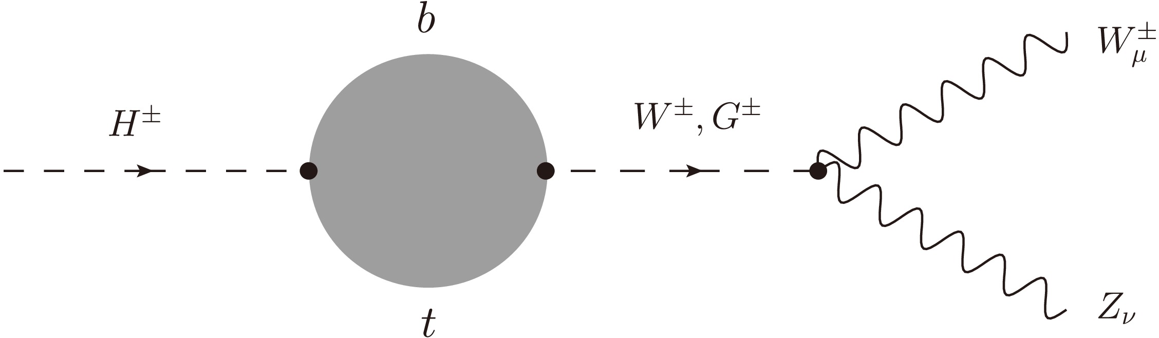
Figure A9. Self-energy Feynman diagram contributions at the external leg
$ H^\pm$ with fermion loops.$ \begin{aligned}[b] \dfrac{ {\cal{T}}^{F}_{1, \text{Self}} }{ g_{Z W^\pm W^\mp} \cdot g_{W^+ \bar{t} \, b} } = \;& \dfrac{ 2 N^C_Q }{ 16\pi^2 \cdot m_{W}^2 \big( m_{H^\pm}^2 - m_{W}^2\big ) } \Bigg\{ s_{W}^2 m_{Z}^2 \big( m_{t}^2 \, g^{R}_{H^- t \bar{b}} - m_{b}^2 \, g^{L}_{H^- t \bar{b}} \big) A_{0} (b) - g^{L}_{H^- t \bar{b}} \, m_{b}^2 \, \Big[ m_{W}^2 \big( m_{Z}^2 - m_{W}^2 \big) - s_{W}^2 m_{H^\pm}^2 m_{Z}^2 \Big]\\&\times \big( B_{0} + B_{1} \big) (H^\pm; b,t) + s_{W}^2 m_{Z}^2 m_{t}^2 g^{R}_{H^- t \bar{b}} \big( m_{t}^2 -m_{b}^2 -m_{H^\pm}^2 \big) B_{0} (H^\pm; b,t) \\ & + m_{t}^2 g^{R}_{H^- t \bar{b}} \Big[ m_{W}^2 \big( m_{W}^2 - m_{Z}^2 \big) - s_{W}^2 m_{H^\pm}^2 m_{Z}^2 \Big] B_{1} (H^\pm; b,t) \Bigg\}, \end{aligned} $
(A41) $ {\cal{T}}^{F}_{2, \text{Self}} = {\cal{T}}^{F}_{3, \text{Self}} = 0. $
(A42) The general couplings involving the Goldstone bosons
$ G^\pm $ and quarks$ f, f' $ exchanging in the loop are given by$ \lambda_{G^- f \bar{f'}} = -i \Big( m_{f'} \, g^{L}_{G^- f \bar{f'}} P_L + m_f \, g^{R}_{G^- f \bar{f'}} P_R \Big) $ , and$ \lambda_{G^+ f' \bar{f}} = -i \Big( m_f \, g^{L}_{G^+ f' \bar{f}} P_L + m_{f'} \, g^{R}_{G^+ f' \bar{f}} P_R \Big) $ . Furthermore, the left- and right-handed couplings satisfy the relations as$ g^{L}_{G^+ f' \bar{f}} = g^{R}_{G^- f \bar{f'}} = -\frac{1}{m_W} \, g_{W^\pm f \bar{f'}} $ and$ g^{R}_{G^+ f' \bar{f}} = g^{L}_{G^- f \bar{f'}} = +\frac{1}{m_W} \, g_{W^\pm f \bar{f'}} $ .$ {\underline{Form\ factors \ {\cal{T}}^{F}_{i, \text{Tad}}}} $ :Regarding to Fig. A10, form factor
$ {\cal{T}}^{F}_{i, \text{Tad}} $ for$ i = 1, 2, 3 $ is expressed into one-loop contributions by pole$ \phi \equiv h, H $ and pole A as follows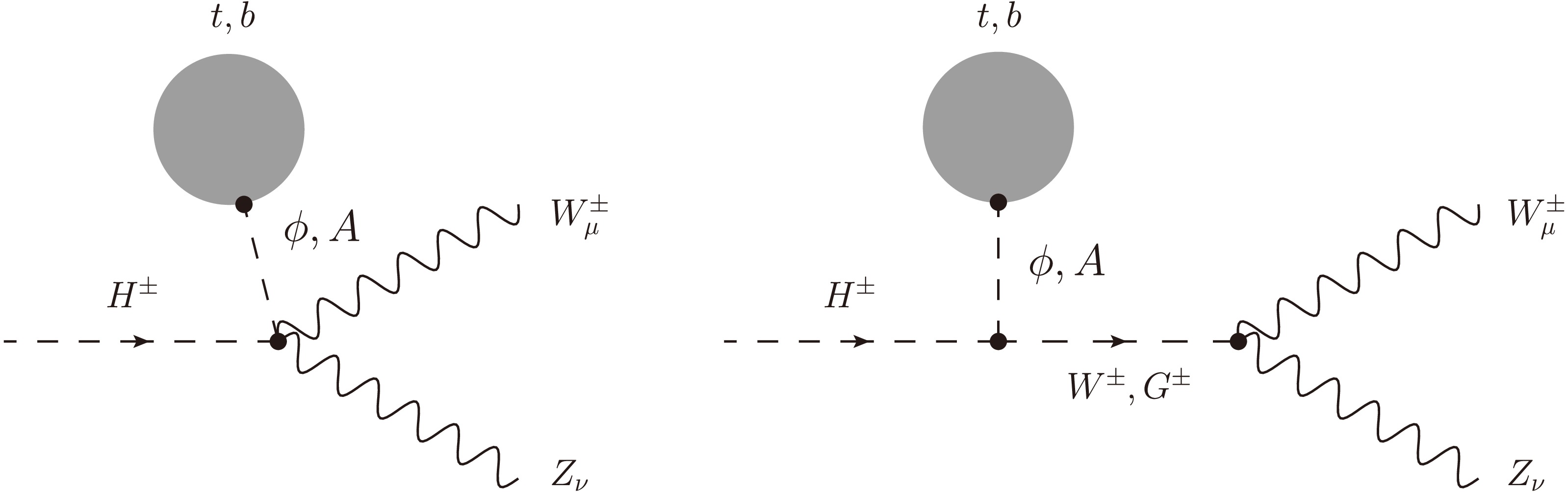
Figure A10. Tadpole Feynman diagram contributions with poles
$ \phi \equiv h, H, A$ for fermion loops.$ {\cal{T}}^{F}_{i, \text{Tad}} = {\cal{T}}^{F, A}_{i, \text{Tad}} + \sum \limits_{\phi = h, H} {\cal{T}}^{F, \phi}_{i, \text{Tad}}. $
(A43) Where the related general couplings for these scalar Higgs ϕ and pseudo-scalar Higgs A with fermion f vertices are introduced with
$ g^{L}_{\phi f \bar{f}} = g^{R}_{\phi f \bar{f}} \equiv g_{\phi f \bar{f}} $ and$ g^{R}_{A f \bar{f}} = - g^{L}_{A f \bar{f}} = g_{A f \bar{f}} $ as follows:$-i \, m_f \big( g^{L}_{\phi f \bar{f}} \, P_L + g^{R}_{\phi f \bar{f}} \, P_R \big) = -i \, m_f \, g_{\phi f \bar{f}}$ , and$ m_f \big( g^{L}_{A f \bar{f}} \, P_L + g^{R}_{A f \bar{f}} \, P_R \big) = m_f \, g_{A f \bar{f}} \, \gamma_5 $ . Therefore these all form factors at pole A by an analytical relation$ g^{L}_{A f \bar{f}} + g^{R}_{A f \bar{f}} = 0 $ and ones for$ i = 2, 3 $ at pole ϕ have no contribution for fermion tadpole diagrams,$ {\cal{T}}^{F, A}_{1, \text{Tad}} = {\cal{T}}^{F, A / \phi}_{2, \text{Tad}} = {\cal{T}}^{F, A / \phi}_{3, \text{Tad}} = 0 $
(A44) and thus, the remaining form factor contributed from only pole ϕ is reading as follows
$\begin{aligned}[b] {\cal{T}}^{F, \phi}_{1, \text{Tad}} =\;& \dfrac{ N^C_Q }{ 16\pi^2 \cdot m_{\phi}^2 \big(m_{H^\pm}^2 - m_{W}^2 \big) } \\& \times \Big[ \big( m_{H^\pm}^2 -m_{W}^2 \big) g_{\phi H^-W^+Z} \\& + \frac{s_W^2}{c_W^2} \big( m_{\phi}^2 -m_{H^\pm}^2 \big) \; g_{\phi H^- W^+} \cdot g_{Z W^\pm W^\mp} \\ & + \big( m_{Z}^2 - m_{W}^2 \big) g_{\phi H^- W^+} \cdot g_{Z W^\pm W^\mp} \Big] \times \\ & \times \Big[ 4 m_{b}^2 \, g_{\phi b \bar{b}} \, A_{0} (b) + 4 m_{t}^2 \, g_{\phi t \bar{t}} \, A_{0} (t) \Big]. \end{aligned}$
(A45) -
The conventions for one-loop one-, two-, and three-point tensor integrals with rank P, following Refs. [70, 59, 71], are given by
$ \{A; B; C\}^{\mu_1\mu_2\cdots \mu_P}= (\mu^2)^{2-d/2} \int \frac{{\rm d}^dk}{(2\pi)^d} \dfrac{k^{\mu_1}k^{\mu_2} \cdots k^{\mu_P}}{\{D_1; D_1 D_2; D_1 D_2 D_3\}}. $
(A1) Here,
$ D_j^{-1} $ ($ j = 1, \cdots, 3 $ ) are the Feynman propagators defined as$ D_j = (k + q_j)^2 - m_j^2 + {\rm i}\rho, $
(A2) where
$ q_j = \sum\limits_{i=1}^j p_i $ ,$ p_i $ are the external momenta, and$ m_j $ are the internal masses in the loops. Dimensional regularization for one-loop integrals is performed in a space–time dimension$ d = 4 - 2\varepsilon $ (the UV-divergent part is isolated as$ C_{UV} = 1/\varepsilon + \log(4\pi) - \Gamma_E $ ,$ \Gamma_E $ is the Euler–Mascheroni constant). In the above expressions, the parameter$ \mu^2 $ serves as the renormalization scale. Explicit reduction formulas for one-, two-, and three-point tensor integrals up to rank$ P = 3 $ are given in Ref. [70].$ A^{\mu} = 0, $
(A3) $ A^{\mu\nu} = g^{\mu\nu} A_{00}, $
(A4) $ A^{\mu\nu\rho} = 0, $
(A5) $ B^{\mu} = q^{\mu} B_1, $
(A6) $ B^{\mu\nu} = g^{\mu\nu} B_{00} + q^{\mu}q^{\nu} B_{11}, $
(A7) $ B^{\mu\nu\rho} = \{g, q\}^{\mu\nu\rho} B_{001} + q^{\mu}q^{\nu}q^{\rho} B_{111}, $
(A8) $ C^{\mu} = q_1^{\mu} C_1 + q_2^{\mu} C_2 = \sum\limits_{i=1}^2q_i^{\mu} C_i, $
(A9) $ C^{\mu\nu} = g^{\mu\nu} C_{00} + \sum\limits_{i,j=1}^2q_i^{\mu}q_j^{\nu} C_{ij}, $
(A10) $ C^{\mu\nu\rho} = \sum\limits_{i=1}^2 \{g,q_i\}^{\mu\nu\rho} C_{00i}+ \sum\limits_{i,j,k=1}^2 q^{\mu}_i q^{\nu}_j q^{\rho}_k C_{ijk}. $
(A11) The detailed expressions for these form factors in the general
$ R_{\xi} $ gauge are given in the following paragraphs. In the analytical expressions below, we have used the notations given as follows.$ A_{ij\cdots}(P) = A_{ij\cdots}(M_P^2), $
(A12) $ B_{ij\cdots}(p^2; P_1, P_2) = B_{ij\cdots}(p^2; M_{P_1}^2,M_{P_2}^2 ), $
(A13) $\begin{aligned}[b]& C_{ij\cdots}(p_1^2, p_2^2, p_3^2; P_1, P_2,P_3) = C_{ij\cdots}(p_1^2, p_2^2, p_3^2; M_{P_1}^2, M_{P_2}^2, M_{P_3}^2). \end{aligned} $
(A14) The analytic formulas for all form factors are expressed in terms of PV-functions using the adopted shorthand notations as presented below in the following paragraphs.
${\underline{Form\ factors\ {\cal{T}}^{B}_{i, \text{Trig}} } }$ :The form factor
$ {\cal{T}}^{B}_{i,\text{Trig}} $ ($ i = 1,2,3 $ ) is expressed in terms of the main contributions involving scalar Higgs bosons$ \phi \equiv h, H $ , together with charged particles such as$ H^\pm, W^\pm, G^\pm $ , and neutral particles including$ A, Z, G^0 $ circulating in the loop.$ {\cal{T}}^{B}_{i, \text{Trig}} = \sum \limits_{\phi = h, H} \Big( {\cal{T}}^{B, \phi-A}_{i, \text{Trig}} + {\cal{T}}^{B, \phi-H^\pm}_{i, \text{Trig}} + {\cal{T}}^{B, \phi-W^\pm}_{i, \text{Trig}} + {\cal{T}}^{B, \phi-Z}_{i, \text{Trig}} + {\cal{T}}^{B, \phi-W^\pm Z}_{i, \text{Trig}} \Big). $
(A15) Each contribution of
$ {\cal{T}}^{B}_{1, \text{Trig}} $ and$ {\cal{T}}^{B}_{2, \text{Trig}} $ is calculated from the corresponding Figs. A1, A2, A3, A4 and A5, respectively. In contrast, the form factor$ {\cal{T}}^{B}_{3, \text{Trig}} $ makes no contribution in one-loop boson-exchanging diagrams. In Fig. A1, the contribution in first for exchanging of ϕ and the pseudo-scalar Higgs A are given as follows.
Figure A1. One-loop triangle Feynman diagrams with
$\phi = h, H, A$ , together with$H^\pm$ or$W^\pm$ propagating in the loop.
Figure A2. One-loop triangle Feynman diagrams with
$\phi = h, H$ and$H^\pm$ in the loop.
Figure A3. One-loop triangle diagrams with
$\phi = h, H$ and$W^\pm$ in the loop.
Figure A4. One-loop triangle diagrams with
$\phi = h, H$ and Z as internal lines in the loop.
Figure A5. One-loop triangle Feynman diagrams with
$ \phi = h, H$ exchanging in association with$W^\pm $ and Z contributions in the loop.$ \begin{aligned}[b] \dfrac{ {\cal{T}}^{B, \phi-A}_{1, \text{Trig}} }{ g_{A H^- W^+} \cdot g_{\phi A Z} } =\;& - \dfrac{ g_{\phi W^\pm W^\mp} }{ 8\pi^2 \cdot m_W^2 } \big[ \big( m_{A}^2 +m_{H^\pm}^2 -\xi_{W} m_{W}^2 \big) C_{00} + 2 m_{H^\pm}^2 C_{002} + \big( m_{H^\pm}^2 -m_{W}^2 +m_{Z}^2 \big) C_{001} \big] (Z,W,H^\pm; A,\phi,\xi_W W ) \\& + \dfrac{ g_{\phi W^\pm W^\mp} }{ 8\pi^2 \cdot m_W^2 } \big[ 2 m_{H^\pm}^2 C_{00} + \big( m_{H^\pm}^2 -m_{W}^2 +m_{Z}^2 \big) C_{001} + 2 m_{H^\pm}^2 C_{002} \big] (Z,W,H^\pm;A,\phi,W) \\& - \dfrac{ g_{\phi H^\pm H^\mp} }{ 4\pi^2 } C_{00}(Z,H^\pm,W;A, \phi,H^\pm), \end{aligned} $
(A16) $\begin{aligned}[b] \dfrac{ {\cal{T}}^{B, \phi-A}_{2, \text{Trig}} }{ g_{A H^- W^+} \cdot g_{\phi A Z} } =\;& \dfrac{ g_{\phi W^\pm W^\mp} }{8\pi^2 \cdot m_W^2} \Big[ 2 \big( C_{00} + C_{001} \big) + \big( m_{H^\pm}^2 -m_{W}^2 +m_{Z}^2 \big) C_{112} + \big( 3 m_{H^\pm}^2 -m_{W}^2 +m_{Z}^2 \big) \big( C_{12} + C_{122} \big) + 4 \big( m_{H^\pm}^2 C_{22} + C_{002} \big) \\ & + 2 \big( m_{H^\pm}^2 -m_{W}^2 \big) C_{2} + 2 m_{H^\pm}^2 C_{222} \Big] (Z,W,H^\pm; A,\phi,W) + \dfrac{ g_{\phi W^\pm W^\mp} }{8\pi^2 \cdot m_W^2} \Big[ \big( m_{W}^2 -m_{Z}^2 -3 m_{H^\pm}^2 \big) C_{122}\\ & - 2 \big( C_{00} + C_{001} + 2 C_{002} \big) - \big( m_{A}^2 +m_{H^\pm}^2 -\xi_{W} m_{W}^2 \big) C_{2} - \big( m_{H^\pm}^2 -m_{W}^2 +m_{Z}^2 \big) C_{112}\\ & - \Big( m_{A}^2 +2 m_{H^\pm}^2 - \big( \xi_{W}+1 \big) m_{W}^2 + m_{Z}^2 \Big) C_{12} - 2 m_{H^\pm}^2 C_{222} \\ &- \big( m_{A}^2 +3 m_{H^\pm}^2 -\xi_{W} m_{W}^2 \big) C_{22} \Big](Z,W, H^\pm; A, \phi, \xi_W W) + \dfrac{ g_{\phi H^\pm H^\mp} }{4\pi^2} C_{12} (Z,H^\pm,W; A, \phi, H^\pm), \end{aligned} $
(A17) $ \dfrac{ {\cal{T}}^{B, \phi-A}_{3, \text{Trig}} }{ g_{A H^- W^+} \cdot g_{\phi A Z} } = 0. $
(A18) Following Fig. A2, the one-loop contributions from the exchange of ϕ and the charged Higgs
$ H^\pm $ are expressed as follows.$ \begin{aligned}[b]& \dfrac{ {\cal{T}}^{B, \phi-H^\pm}_{1, \text{Trig}} }{ 16\pi^2 \cdot g_{\phi H^\pm H^\mp} } = g_{\phi H^-W^+Z} \cdot B_{0}(H^\pm;\phi,H^\pm)\\&\quad - 4 \, g_{\phi H^- W^+} \cdot g_{Z H^\pm H^\mp} \, C_{00}(W,Z,H^\pm;\phi,H^\pm, H^\pm), \end{aligned}$
(A19) $\begin{aligned}[b] \dfrac{ {\cal{T}}^{B, \phi-H^\pm}_{2, \text{Trig}} }{ 16\pi^2 \cdot g_{\phi H^\pm H^\mp} } =\;& -4 g_{\phi H^- W^+} \cdot g_{Z H^\pm H^\mp} \big( C_{2} + C_{12} + C_{22} \big)\\&\times (W,Z, H^\pm; \phi,H^\pm, H^\pm), \end{aligned} $
(A20) $ \dfrac{ {\cal{T}}^{B, \phi-H^\pm}_{3, \text{Trig}} }{ 16\pi^2 \cdot g_{\phi H^\pm H^\mp} } = 0. $
(A21) From Fig. A3, we obtain the form factors involving the neutral scalar Higgs boson ϕ in association with the vector boson
$ W^\pm $ and the Goldstone bosons$ G^\pm $ in the loop. The factor is given by$ \begin{aligned}[b] \dfrac{ {\cal{T}}^{B, \phi-W^\pm}_{1, \text{Trig}} } { g_{\phi W^\pm W^\mp} } = \;&\dfrac{ g_{\phi H^- W^+} \cdot g_{Z W^\pm W^\mp} }{32\pi^2 \cdot m_{W}^4} \Big\{ 2 m_{W}^2 \Big[ A_{0}(W) - A_{0}(\xi_W W) \Big] + \Big[ 2 m_{W}^2 \big( m_{H^\pm}^2 -m_{\phi}^2 +m_{Z}^2 -m_{W}^2 \big) B_{0} - 2 m_{Z}^2 B_{00} \Big] (Z; W,\xi_{W} W) \\& + \Big[ 2 m_{W}^2 \big( m_{\phi}^2 -m_{H^\pm}^2 -m_{Z}^2 \big) B_{0} + 2 \big( m_{Z}^2 -m_{W}^2 \big) B_{00} \Big](Z; W, W) + 2 m_{W}^2 B_{00}(Z;\xi_{W} W, \xi_{W} W ) \\ &- s_{W}^2 m_{Z}^2 \big( m_{\phi}^2 -m_{H^\pm}^2 \big) B_{0} (H^\pm; \phi, \xi_W W) + 2 m_{W}^2 \Big[ \big( m_{H^\pm}^2 - m_{\phi}^2 \big) \big( m_{H^\pm}^2 +m_{W}^2 -m_{Z}^2 \big) C_{2} + 2 m_{W}^2 \big( m_{H^\pm}^2 -m_{\phi}^2 \big) C_{1} \\ & - m_{\phi}^2 \big( m_{\phi}^2 -m_{H^\pm}^2 \big) C_{0} \Big] (W,Z, H^\pm;\phi,W, \xi_W W) + 2 m_{W}^2 \Big[ \big( m_{W}^2 -m_{H^\pm}^2 -m_{\phi}^2 \big) C_{00} - \big( m_{H^\pm}^2 +m_{W}^2 -m_{Z}^2 \big) C_{002} \\ & - 2 m_{H^\pm}^2 C_{001} \Big](H^\pm, Z, W; \phi,W, \xi_W W) \Big\} + \dfrac{ g_{\phi H^- W^+} \cdot g_{Z W^\pm W^\mp} }{32\pi^2 \cdot m_{W}^4} \Big\{ 2 m_{W}^2 \Big[ \big( m_{H^\pm}^2 +m_{W}^2 -m_{Z}^2 \big) C_{001} + 2 m_{H^\pm}^2 C_{002} \Big] \\ & + 2 m_{W}^2 \Big[ m_{\phi}^4 - m_{\phi}^2 \big( m_{H^\pm}^2 +m_{Z}^2 \big) - \big( m_{H^\pm}^2 -m_{W}^2 \big) \big( m_{W}^2 -m_{Z}^2 \big) \Big] C_{0} + 2 \Big[ m_{\phi}^2 \big( m_{Z}^2 -m_{W}^2 \big) - m_{Z}^2 \big( m_{H^\pm}^2 +m_{W}^2 \big) \\ &+ m_{W}^2 \big( 3 m_{H^\pm}^2 +m_{W}^2 \big) \Big] C_{00} + 2 m_{W}^4 \big( 2 m_{\phi}^2 -m_{H^\pm}^2 -m_{W}^2 -m_{Z}^2 \big) C_{1} + 2 m_{W}^2 \Big[ m_{\phi}^2 \big( m_{H^\pm}^2 +m_{W}^2 -m_{Z}^2 \big)\\ & + m_{H^\pm}^2 \big( m_{Z}^2 -m_{H^\pm}^2 \big) + m_{W}^2 \big( m_{Z}^2 -m_{W}^2 \big) \Big] C_{2} \Big\} (W,Z,H^\pm;\phi, W, W) \\& - \dfrac{ g_{\phi H^- W^+ Z} }{16\pi^2 \cdot m_{W}^2} \Big[ \big( m_{W}^2 B_{0} - B_{00} \big) (W;\phi,W) + B_{00} (W,\phi,\xi_W W) \Big], \end{aligned} $
(A22) $ \begin{aligned}[b] \dfrac{ {\cal{T}}^{B, \phi-W^\pm}_{2, \text{Trig}} } { g_{\phi W^\pm W^\mp} } =\;& - \dfrac{ g_{\phi H^- W^+} \cdot g_{Z W^\pm W^\mp} }{8\pi^2 \cdot m_{W}^2} \Big\{ \big( B_{0} + B_{1} \big) (Z;W,\xi_{W} W ) + B_{1}(Z;W, W) \Big\} - \dfrac{ g_{\phi H^- W^+} \cdot g_{Z W^\pm W^\mp} }{16\pi^2 \cdot m_{W}^4} \Big\{ 4 m_{W}^4 C_{1} \\&+ \Big[ m_{W}^2 \big( 3 m_{\phi}^2 -m_{H^\pm}^2 +m_{W}^2 \big) - m_{Z}^2 \big( m_{\phi}^2 -m_{H^\pm}^2 +m_{W}^2 \big) \Big] C_{2} + \Big[ m_{\phi}^2 \big( m_{W}^2 -m_{Z}^2 \big) + m_{H^\pm}^2 \big( m_{Z}^2 -2 m_{W}^2 \big) \Big] C_{12}\\& + 2 m_{W}^2 \big( C_{00} - C_{001} - 2 C_{002} \big) + \big( m_{W}^2-m_{Z}^2 \big) \big( m_{\phi}^2 -m_{H^\pm}^2 -m_{W}^2 \big) C_{22} - m_{W}^2 \big( m_{H^\pm}^2 +m_{W}^2 -m_{Z}^2 \big) C_{112} \\ & + m_{W}^2 \big( m_{Z}^2 -m_{W}^2 -3 m_{H^\pm}^2 \big) C_{122} - 2 m_{H^\pm}^2 m_{W}^2 C_{222} \Big\} (W,Z,H^\pm;\phi,W,W ) - \dfrac{ g_{\phi H^- W^+} \cdot g_{Z W^\pm W^\mp} }{16\pi^2 \cdot m_{W}^4} \\& \times \Big\{ m_{W}^2 \big( m_{W}^2 -m_{\phi}^2 -m_{H^\pm}^2 \big) C_{1} + m_{W}^2 \big( m_{\phi}^2 -m_{H^\pm}^2 -m_{W}^2 \big) C_{11} + m_{W}^2 \big( m_{\phi}^2 -2 m_{W}^2 +m_{Z}^2 \big) C_{12} - 2 m_{W}^2 \big( C_{00} - C_{002} - 2 C_{001} \big)\\ & + m_{W}^2 \big( m_{W}^2 -m_{Z}^2 +3 m_{H^\pm}^2 \big) C_{112} + m_{W}^2 \big( m_{H^\pm}^2 +m_{W}^2 -m_{Z}^2 \big) C_{122} + 2 m_{H^\pm}^2 m_{W}^2 C_{111} \Big\} (H^\pm,Z, W; \phi, W, \xi_{W} W), \end{aligned}$
(A23) $ \dfrac{ {\cal{T}}^{B, \phi-W^\pm}_{3, \text{Trig}} }{ g_{\phi W^\pm W^\mp} } = 0. $
(A24) As shown in Fig. A4, the corresponding one-loop form factors, with both Higgs bosons ϕ and the vector boson Z exchanged in the loop given as follows.
$\begin{aligned}[b] \dfrac{ {\cal{T}}^{B, \phi-Z}_{1, \text{Trig}} } { g_{\phi ZZ} } = \;& - \dfrac{ g_{\phi H^- W^+ Z} }{ 16\pi^2 \cdot m_{Z}^2} \Big[ \big( m_{Z}^2 B_{0} - B_{00} \big) (Z;\phi,Z)\\ & + B_{00} (Z;\phi,\xi_Z Z) \Big]- \dfrac{ g_{\phi H^- W^+} \cdot g_{Z H^\pm H^\mp} }{ 8\pi^2 \cdot m_{Z}^2} \\& \times \Big[ B_{00} (Z; \phi,Z) - B_{00} (Z;\phi,\xi_Z Z) \\& - m_{Z}^2 C_{00} (W,H^\pm,Z;\phi,H^\pm,Z) \Big], \end{aligned} $
(A25) $\begin{aligned}[b]\\[-12pt] \dfrac{ {\cal{T}}^{B, \phi-Z}_{2, \text{Trig}} } { g_{\phi ZZ} } =\;&- \dfrac{ g_{\phi H^- W^+} \cdot g_{Z H^\pm H^\mp} }{16\pi^2} \big( 4 C_{2} + 2 C_{12} \big)\\& \times (W,H^\pm,Z;\phi,H^\pm,Z), \end{aligned} $
(A26) $ \dfrac{ {\cal{T}}^{B, \phi-Z}_{3, \text{Trig}} } { g_{\phi ZZ} } = 0. $
(A27) In Fig. A5, the form factors corresponding to the neutral scalar Higgs ϕ accompanied by both the vector bosons
$ W^\pm $ and Z and the Goldstone bosons$ G^\pm $ and$ G^0 $ in the loop are represented as follows.$ \begin{aligned}[b] \dfrac{ {\cal{T}}^{B, \phi-W^\pm Z}_{1, \text{Trig}} } { g_{\phi ZZ} } =\;& \dfrac{ g_{\phi H^- W^+} \cdot g_{Z W^\pm W^\mp} }{16\pi^2} \xi_{W} B_{0} (Z; \phi,Z) + \dfrac{ g_{\phi H^- W^+} \cdot g_{Z W^\pm W^\mp} }{16\pi^2 \cdot m_{W}^2 m_{Z}^2} \Big\{ \big[ c_{W}^2 m_{Z}^2 \big( m_{\phi}^2 -m_{H^\pm}^2 \big) \\ &+ m_{W}^2 \big( 2 m_{H^\pm}^2 - \xi_{W} m_{W}^2 \big) \big] C_{00} + m_{W}^2 \big[ \big( m_{H^\pm}^2 -m_{W}^2 +m_{Z}^2 \big) C_{002} + 2 m_{H^\pm}^2 C_{001} \big] \Big\} (H^\pm, W, Z; \phi,\xi_{W} W, \xi_{Z} Z ) \\& + \dfrac{ g_{\phi H^- W^+} \cdot g_{Z W^\pm W^\mp} }{16\pi^2 \cdot m_{W}^2 m_{Z}^2} \Bigg\{ m_{Z}^2 \Big[ m_{H^\pm}^2 \big[ m_{W}^2 \big( 2-3 \xi_{W} \big) + m_{Z}^2 \big( s_{W}^2-2 \big) + 2 m_{H^\pm}^2 \big] - m_{\phi}^2 m_{Z}^2 s_{W}^2 + \xi_{W} m_{W}^2 \big[ m_{W}^2 \big( \xi_{W}-1 \big) + m_{Z}^2 \big] \Big] C_{0} \\& - m_{Z}^2 \Big[ m_{H^\pm}^2 \big( 2 m_{W}^2 + 2 m_{Z}^2- 3 m_{H^\pm}^2 \big) + 2 \xi_{W} m_{W}^2 \big( m_{H^\pm}^2 - m_{W}^2 \big) + \big( m_{W}^2 -m_{Z}^2 \big)^2 \Big] C_{1} + \Big[ m_{Z}^2 \big( m_{\phi}^2 s_{W}^2 +2 m_{W}^2 -2 m_{Z}^2 \big) \\ & - m_{H^\pm}^2 \big[ 2 m_{W}^2 + m_{Z}^2 \big( s_{W}^2-4 \big) \big] + \xi_{W} m_{W}^2 \big( m_{W}^2 -m_{Z}^2 \big) \Big] C_{00} - m_{Z}^2 \Big[ m_{H^\pm}^2 \big( 2 m_{W}^2 + 2 m_{Z}^2 -3 m_{H^\pm}^2 \big) + \big( m_{W}^2 -m_{Z}^2 \big)^2 \Big] C_{12} \\ & + m_{Z}^2 \Big[ \xi_{W} m_{W}^2 \big( m_{Z}^2 -m_{W}^2 -3 m_{H^\pm}^2 \big) + 4 m_{H^\pm}^2 \big( m_{H^\pm}^2 +m_{W}^2 -m_{Z}^2 \big) \Big] C_{2} + \big( m_{Z}^2 -m_{W}^2 \big) \Big[ 2 m_{H^\pm}^2 C_{002} + \big( m_{H^\pm}^2 -m_{W}^2 +m_{Z}^2 \big) C_{001} \Big] \\& + m_{Z}^2 \Big[ \big( m_{H^\pm}^2 -m_{W}^2 +m_{Z}^2 \big) \big( m_{H^\pm}^2 -m_{W}^2 -m_{Z}^2 \big) C_{11} + 2 m_{H^\pm}^2 \big( m_{H^\pm}^2 +m_{W}^2 -m_{Z}^2 \big) C_{22} \Big] \Bigg\} (Z,W,H^\pm; \phi,Z, \xi_W W)\\& + \dfrac{ g_{\phi H^- W^+} \cdot g_{Z W^\pm W^\mp} }{16\pi^2 \cdot m_{W}^2} \times\Bigg\{ 2 \big( m_{H^\pm}^2 +m_{W}^2 -m_{Z}^2 \big) \Big[ \big( m_{W}^2 - m_{H^\pm}^2 \big) C_{0} - C_{00} \Big] + \Big[ m_{H^\pm}^2 \big( 2 m_{W}^2 + 2 m_{Z}^2 -3 m_{H^\pm}^2 \big) + \big( m_{W}^2 -m_{Z}^2 \big)^2 \Big] \\ &\times\big( C_{2} + C_{12} \big) + \big( m_{H^\pm}^2 -m_{W}^2 +m_{Z}^2 \big) \Big[ \big( m_{W}^2 +m_{Z}^2 -m_{H^\pm}^2 \big) C_{22} - C_{002} \Big] - 2 m_{H^\pm}^2 \Big[ \big( m_{H^\pm}^2 +m_{W}^2 -m_{Z}^2 \big) \big( 2 C_{1} + C_{11} \big) \\ &+ \big( C_{00} + C_{001} \big) \Big] \Bigg\}\times (H^\pm, W, Z; \phi, W, Z), \end{aligned} $
(A28) $ \begin{aligned}[b] \dfrac{ {\cal{T}}^{B, \phi-W^\pm Z}_{2, \text{Trig}} }{ g_{\phi ZZ} } = \;& \dfrac{ g_{\phi H^- W^+} \cdot g_{Z W^\pm W^\mp} }{16\pi^2 \cdot m_{W}^2 m_{Z}^2} \Bigg\{ \Big[ m_{Z}^2 c_{W}^2 \big( m_{\phi}^2 - m_{H^\pm}^2 \big) + m_{W}^2 \big( 2 m_{H^\pm}^2 - \xi_{W} m_{W}^2 \big) \Big] C_{1} + \Big[ m_{Z}^2 c_{W}^2 \big( m_{\phi}^2 - m_{H^\pm}^2 \big) + m_{W}^2 \big( 4 m_{H^\pm}^2 - \xi_{W} m_{W}^2 \big) \Big] C_{11} \\& + \Big[ m_{Z}^2 \big( c_{W}^2 m_{\phi}^2 + m_{W}^2 \big) - m_{H^\pm}^2 \big( c_{W}^2 m_{Z}^2 - 3 m_{W}^2 \big) - m_{W}^4 \big( \xi_{W} + 1 \big) \Big] C_{12} + 2m_{W}^2 m_{H^\pm}^2 C_{111} + m_{W}^2 \big( 3 m_{H^\pm}^2 -m_{W}^2 +m_{Z}^2 \big) C_{112} \\& + m_{W}^2 \big( m_{H^\pm}^2 -m_{W}^2 +m_{Z}^2 \big) C_{122} + 2 m_{W}^2 \big( C_{00} + 2 C_{001} + C_{002} \big) \Bigg\} (H^\pm, W, Z; \phi,\xi_{W} W,\xi_{Z} Z ) \\ & + \dfrac{ g_{\phi H^- W^+} \cdot g_{Z W^\pm W^\mp} }{16\pi^2 \cdot m_{W}^2 m_{Z}^2} \Bigg\{ \big( m_{Z}^2 -m_{W}^2 \big) \Big[ 2 C_{00} + 2 C_{001} + 4 C_{002} + 2 m_{H^\pm}^2 C_{222} + \big( m_{H^\pm}^2 -m_{W}^2 +m_{Z}^2 \big) C_{112} \\ &+ \big( 3 m_{H^\pm}^2 -m_{W}^2 +m_{Z}^2 \big) C_{122} \Big] + \Big[ m_{\phi}^2 m_{Z}^2 s_{W}^2 - m_{H^\pm}^2 \big( m_{W}^2 - m_{Z}^2 \big) + \xi_{W} m_{W}^2 \big( m_{W}^2 -m_{Z}^2 \big) \Big] C_{2} + \Big[ m_{\phi}^2 m_{Z}^2 s_{W}^2 - 3 m_{H^\pm}^2 \big( m_{W}^2 - m_{Z}^2 \big)\\ & + \xi_{W} m_{W}^2 \big( m_{W}^2 -m_{Z}^2 \big) \Big] C_{22} - \Big[ 3 m_{H^\pm}^2 m_{W}^2 - m_{Z}^2 \big( m_{\phi}^2 s_{W}^2 + m_{Z}^2 \big) + m_{H^\pm}^2 m_{Z}^2 \big( s_{W}^2-3 \big) - m_{W}^4 \big( \xi_{W}+1 \big) \\ &+ m_{W}^2 m_{Z}^2 \big( \xi_{W}+2 \big) \Big] C_{12} \Bigg\} (Z,W,H^\pm; \phi,Z,\xi_W W) + \dfrac{ g_{\phi H^- W^+} \cdot g_{Z W^\pm W^\mp} }{16\pi^2 \cdot m_{W}^2 } \Bigg\{ \big( m_{W}^2 -m_{Z}^2 -3 m_{H^\pm}^2 \big) \big( C_{12} + C_{112} \big) \\ & - \big( m_{H^\pm}^2 -m_{W}^2 +m_{Z}^2 \big) C_{122} + 2 m_{W}^2 \big( C_{1} + 2 C_{2} \big) - 2 m_{H^\pm}^2 \big( C_{1} + 2 C_{11} + C_{111} \big) - 2 \big( C_{00}\\ & + 2 C_{001} + C_{002} \big) \Bigg\} (H^\pm,W,Z; \phi,W, Z), \\ \dfrac{ {\cal{T}}^{B, \phi-W^\pm Z}_{3, \text{Trig}} } { g_{\phi ZZ} } =\;& 0. \end{aligned} $
(A29) ${\underline{Form\ factors \ {\cal{T}}^{B}_{i, \text{Self}}}} $ :Following Fig. A6, the form factors
$ {\cal{T}}^{B}_{i, \text{Self}} $ for$ i = 1, 2, 3 $ are decomposed into two contributions from one-point$ (1P) $ and two-point$ (2P) $ Feynman diagrams. These factors are expressed as follows.
Figure A6. Self-energy Feynman diagram contributions to the external leg
$ H^\pm$ .$ {\cal{T}}^{B}_{i, \text{Self}} = {\cal{T}}^{B}_{i, \text{Self} - 1P} + \sum \limits_{\phi = h, H} \Big( {\cal{T}}^{B, \phi-H^\pm}_{i, \text{Self} - 2P} + {\cal{T}}^{B, \phi-W^\pm}_{i, \text{Self} - 2P} \Big) $
(A30) In this equation, the form factors above for
$ i = 1 $ are obtained as follows.$ \begin{aligned}[b] \dfrac{ {\cal{T}}^{B}_{1, \text{Self} - 1P} }{ g_{Z W^\pm W^\mp} } =\;& \dfrac{m_{W} s_{W}^2}{ 32\pi^2 \cdot c_{W}^2 \big(m_{H^\pm}^2 - \xi m_{W}^2\big) } \times \Bigg\{ g_{G^0 G^0 H^- G^+} \, A_0 (\xi_{Z} Z) + 2 g_{G^+ G^- H^- G^+} \, A_0 (\xi_{W} W) \\& + g_{A A H^- G^+} \, A_0 (A) + 2 g_{H^+ H^- H^- G^+} \, A_0 (H^\pm) + g_{h h \, H^- G^+} \, A_0 (h) + g_{H H \, H^- G^+} \, A_0 (H) \Bigg\}, \end{aligned}$
(A31) $ \begin{aligned}[b] \dfrac{ {\cal{T}}^{B, \phi-H^\pm}_{1, \text{Self} - 2P} }{ g_{Z W^\pm W^\mp} } =\;& - \dfrac{ g_{\phi H^- W^+} \cdot g_{\phi H^\pm H^\mp} }{ 16\pi^2 \cdot m_{W}^2 \big( m_{H^\pm}^2 - \xi_{W} m_{W}^2 \big)} \Bigg\{ 2 \xi_{W} m_{W}^2 \big( m_{W}^2 -m_{Z}^2 \big) B_{1}(H^\pm; \phi, H^\pm)\\ & + \Big[ m_{Z}^2 s_{W}^2 \big( m_{H^\pm}^2 - m_{\phi}^2 \big) + \xi_{W} m_{W}^2 \big( m_{W}^2 -m_{Z}^2 \big) \Big] B_{0}(H^\pm; \phi, H^\pm) \Bigg\}, \end{aligned} $
(A32) $ \begin{aligned}[b] \dfrac{{\cal{T}}^{B, \phi-W^\pm}_{1, \text{Self} - 2P} }{ g_{Z W^\pm W^\mp} } =\;& - \dfrac{ g_{\phi H^- W^+} \cdot g_{\phi W^\pm W^\mp} }{ 32\pi^2 \cdot m_{W}^4 \big( m_{H^\pm}^2 - \xi_{W} m_{W}^2 \big)} \times \Bigg\{ s_{W}^2 m_{Z}^2 \Big[ \big( m_{\phi}^2 -m_{H^\pm}^2 \big) A_{0} (W) - \big( m_{\phi}^2 -m_{H^\pm}^2 +\xi_{W} m_{W}^2 \big) A_{0} (\xi_{W} W) \Big] \\& + \big( m_{\phi}^2 -m_{H^\pm}^2 \big) \Big[ s_{W}^2 m_{H^\pm}^2 m_{Z}^2 + \xi_{W} m_{W}^2 \big( m_{W}^2 -m_{Z}^2 \big) \Big] B_{0} (H^\pm; \phi, \xi_{W} W) + 2 m_{W}^2 \Big[ \xi_{W} \big( m_{W}^2 -m_{Z}^2 \big) \big( m_{H^\pm}^2 +m_{W}^2 -m_{\phi}^2 \big) \\ & + s_{W}^2 m_{H^\pm}^2 m_{Z}^2 \Big] B_{1} (H^\pm; \phi,W) + s_{W}^2 m_{Z}^2 \Big[ \big( m_{\phi}^2 -m_{H^\pm}^2 \big)^2 - m_{W}^2 \big( m_{\phi}^2 +m_{H^\pm}^2 \big) \Big] B_{0} (H^\pm; \phi,W) \\& - 2 \xi_{W} m_{W}^2 \big( m_{W}^2 -m_{Z}^2 \big) \big( m_{\phi}^2 -m_{H^\pm}^2 +m_{W}^2 \big) B_{0} (H^\pm; \phi,W) \Bigg\}. \end{aligned} $
(A33) Other values for
$ i = 2, 3 $ have no contribution, or$ {\cal{T}}^{B}_{i, \text{Self} - 1P} = {\cal{T}}^{B, \phi-H^\pm}_{i, \text{Self} - 2P} = {\cal{T}}^{B, \phi-W^\pm}_{i, \text{Self} - 2P} = 0. $
(A34) $ {\underline{Form\ factors \ {\cal{T}}^{B}_{i, \text{Tad}}}} $ :According to Fig. A7, the form factor
$ {\cal{T}}^{B}_{i, \text{Tad}} $ for$ i = 1, 2, 3 $ is expressed in terms of the scalar Higgs$ \phi \equiv h, H $ pole coupling with the bubble diagrams. In these loops, the neutral and pseudo-scalar Higgs particles$ h, H, A $ , the charged Higgs$ H^\pm $ , the vector bosons$ W^\pm $ and Z, the Goldstone bosons$ G^\pm $ and$ G^0 $ , and the corresponding ghost particles$ u_\pm $ and$ u_Z $ are all taken into account. As a result, the factor is given by
Figure A7. Tadpole Feynman diagram contributions with poles
$ \phi \equiv h, H$ .$ {\cal{T}}^{B}_{i, \text{Tad}} = \sum \limits_{\phi = h, H} {\cal{T}}^{B, \phi}_{i, \text{Tad}}. $
(A35) where the form factors are expressed as follows.
$ \begin{aligned}[b] {\cal{T}}^{B, \phi}_{1, \text{Tad}} = \;& - \dfrac{1}{ 64\pi^2 \cdot m_{\phi}^2 \big(m_{H^\pm}^2 - \xi_{W} m_{W}^2 \big) } \times \Big[ g_{\phi H^- W^+ Z} \, \big( m_{H^\pm}^2 - \xi_{W} m_{W}^2 \big) + \big( m_{\phi}^2 -m_{H^\pm}^2 \big) t_{W}^2\; g_{\phi H^- W^+} \cdot g_{Z W^\pm W^\mp} \\& + \xi_{W} \big( m_{Z}^2 -m_{W}^2 \big) g_{\phi H^- W^+} \cdot g_{Z W^\pm W^\mp} \Big] \times \Bigg\{ 4 m_{Z}^2 \, g_{\phi Z Z} + 8 m_{W}^2 \, g_{\phi W^\pm W^\mp} + 2 g_{\phi A A} \; A_{0} (A) + 2 g_{\phi h h} \; A_{0} (h) \\ & + 2 \; g_{\phi H H} \, A_{0} (H) + 4 g_{\phi H^\pm H^\mp} \, A_{0} (H^\pm) - 12 g_{\phi W^\pm W^\mp} A_{0} (W) - 6 g_{\phi Z Z} \, A_{0} (Z) - g_{\phi Z Z} \, \dfrac{m_{\phi}^2}{m_{Z}^2} \; A_{0} (\xi_{Z} Z) \\& - 2 \dfrac{m_{\phi}^2}{m_{W}^2} \, g_{\phi W^\pm W^\mp} \, A_{0} (\xi_{W} W) \Bigg\}, \end{aligned}$
(A36) $ {\cal{T}}^{B, \phi}_{2, \text{Tad}} = {\cal{T}}^{B, \phi}_{3, \text{Tad}} = 0. $
(A37) $ {\underline{Form\ factors \ {\cal{T}}^{F}_{i, \text{Trig}}}} $ :The form factors
$ {\cal{T}}^{F}_{i, \text{Trig}} $ , for$ i = 1, 2, 3 $ as depicted in the corresponding Fig. A8 are given by
Figure A8. One-loop triangle Feynman diagrams with fermion loops.
$ \begin{aligned}[b] \dfrac{{\cal{T}}^{F}_{1, \text{Trig}} }{ g_{W^+ \bar{t} \, b} } =\;& \dfrac{ N^C_Q }{ 8\pi^2} \cdot \Bigg\{ g^{L}_{H^- t \bar{b}} \, m_{b}^2 \, \Big[ g^{L}_{Z t \bar{t}} \, B_{0} (Z; t,t) - \big( g^{R}_{Z b \bar{b}} - g^{L}_{Z b \bar{b}} \big) B_{0} (Z; b,b) \Big] - g^{R}_{H^- t \bar{b}} \, m_{t}^2 \, \Big[ \big( g^{R}_{Z t \bar{t}} - g^{L}_{Z t \bar{t}} \big) B_{0} (Z; t,t) - g^{L}_{Z b \bar{b}} \, B_{0} (Z; b,b) \Big] \\ & - m_{t}^2 \, m_{b}^2 \, \Big[ g^{R}_{Z t \bar{t}} \cdot g^{L}_{H^- t \bar{b}} \, C_{0} (W,Z,H^\pm; b,t,t) + g^{R}_{Z b \bar{b}} \cdot g^{R}_{H^- t \bar{b}} \, C_{0} (Z,H^\pm,W; b,b,t) \Big] \Bigg\} \\ & + \dfrac{ N^C_Q }{ 16\pi^2} \cdot \Bigg\{ - g^{L}_{Z b \bar{b}} \cdot g^{L}_{H^- t \bar{b}} \, m_{b}^2 \, \Big[ 2 \big( m_{W}^2 - m_{t}^2 \big) C_{0} + 4 C_{00} + 2 m_{W}^2 C_{2} - \big( m_{H^\pm}^2 -m_{W}^2 -m_{Z}^2 \big) C_{1} \Big] (Z,H^\pm,W; b,b,t) \\& + g^{L}_{Z t \bar{t}} \cdot g^{L}_{H^- t \bar{b}} \, m_{b}^2 \, \Big[ \big( 2 m_{b}^2 +m_{H^\pm}^2 +m_{W}^2 -m_{Z}^2 \big) C_{0} - 4 C_{00} + \big( m_{H^\pm}^2 +3 m_{W}^2 -m_{Z}^2 \big) C_{1} + \big( 3 m_{H^\pm}^2 +m_{W}^2 -m_{Z}^2 \big) C_{2} \Big]\\&\times (W,Z,H^\pm; b,t,t) - g^{R}_{Z b \bar{b}} \cdot g^{L}_{H^- t \bar{b}} \, m_{b}^2 \, \Big[ \big( 2 m_{t}^2 -m_{H^\pm}^2 -m_{W}^2 +m_{Z}^2 \big) C_{0} + \big( m_{H^\pm}^2 -m_{W}^2 +m_{Z}^2 \big) C_{1} \\ & - \big( m_{H^\pm}^2 +m_{W}^2 -m_{Z}^2 \big) C_{2} \Big] (Z,H^\pm,W; b,b,t) - g^{L}_{Z b \bar{b}} \cdot g^{R}_{H^- t \bar{b}} \, m_{t}^2 \, \Big[ 2 \big( m_{W}^2 - m_{t}^2 \big) C_{0} + 4 C_{00} - 2 \big( m_{H^\pm}^2 -m_{W}^2 \big) C_{1} \\& + \big( m_{H^\pm}^2 +3 m_{W}^2 -m_{Z}^2 \big) C_{2} \Big] (Z,H^\pm,W; b,b,t) + g^{L}_{Z t \bar{t}} \cdot g^{R}_{H^- t \bar{b}} \, m_{t}^2 \, \Big[ 2 m_{b}^2 \, C_{0} - 4 C_{00} + \big( m_{H^\pm}^2 +m_{W}^2 -m_{Z}^2 \big) C_{2} \\& + 2 m_{W}^2 C_{1} \Big] (W,Z,H^\pm; b,t,t) - g^{R}_{Z t \bar{t}} \cdot g^{R}_{H^- t \bar{b}} \, m_{t}^2 \, \Big[ 2 m_{b}^2 \, C_{0} + \big( m_{H^\pm}^2 +m_{W}^2 -m_{Z}^2 \big) C_{1} \\& + 2 m_{H^\pm}^2 C_{2} \Big] (W,Z,H^\pm; b,t,t) \Bigg\}, \end{aligned} $
(A38) $ \begin{aligned}[b] \dfrac{{\cal{T}}^{F}_{2, \text{Trig}} }{ g_{W^+ \bar{t} \, b} } =\;& \dfrac{ N^C_Q }{ 8\pi^2} \cdot \Bigg\{ - g^{L}_{Z t \bar{t}} \cdot g^{L}_{H^- t \bar{b}} \, m_{b}^2 \, \times \big( C_{0} + C_{1} + 3 C_{2} + 2 C_{12} + 2 C_{22} \big) (W,Z,H^\pm; b,t,t) + g^{L}_{H^- t \bar{b}} \, m_{b}^2 \\ & \times \Big[ g^{L}_{Z b \bar{b}} \, \big( C_{1} + 2 C_{12} \big) - g^{R}_{Z b \bar{b}} \, \big( C_{0} + C_{1} + C_{2} \big) \Big] (Z,H^\pm,W; b,b,t) + g^{L}_{Z b \bar{b}} \cdot g^{R}_{H^- t \bar{b}} \, m_{t}^2 \, \big( C_{2} + 2 C_{12} \big) (Z,H^\pm,W; b,b,t) \\ & + g^{R}_{H^- t \bar{b}} \, m_{t}^2 \, \Big[ g^{R}_{Z t \bar{t}} \, C_{1} - g^{L}_{Z t \bar{t}} \, \big( C_{2} + 2 C_{12} + 2 C_{22} \big) \Big] (W,Z,H^\pm; b,t,t) \Bigg\}, \end{aligned} $
(A39) $ \begin{aligned}[b] \dfrac{{\cal{T}}^{F}_{3, \text{Trig}} }{ g_{W^+ \bar{t} \, b} } =\;& \dfrac{ N^C_Q }{ 8\pi^2} \times \Bigg\{ - g^{L}_{Z t \bar{t}} \cdot g^{L}_{H^- t \bar{b}} \, m_{b}^2 \, \big( C_{0} + C_{1} + C_{2} \big) (W,Z,H^\pm; b,t,t) + g^{L}_{H^- t \bar{b}} \, m_{b}^2 \, \Big[ g^{L}_{Z b \bar{b}} \, C_{1} - g^{R}_{Z b \bar{b}} \, \big( C_{0} + C_{1} + C_{2} \big) \Big] (Z,H^\pm,W; b,b,t) \\& - m_{t}^2 g^{R}_{H^- t \bar{b}} \Big( g^{R}_{Z t \bar{t}} \, C_{1} + g^{L}_{Z t \bar{t}} \, C_{2} \Big) (W,Z,H^\pm; b,t,t) - m_{t}^2 g^{R}_{H^- t \bar{b}} g^{L}_{Z b \bar{b}} \, C_{2} (Z,H^\pm,W; b,b,t) \Big] \Bigg\}, \end{aligned} $
(A40) where the color index
$ N^C_Q $ for quarks such as top quark t and bottom quark b exchanging in loop has a value of 3. These related general couplings for these vector boson - fermion vertices are expressed with$ g^{L}_{Z f \bar{f}} = e/(s_{W} c_{W}) \times$ $ (I^3_f - s_{W}^2 Q_f), \,\,\, g^{R}_{Z f \bar{f}} = e/(s_{W} c_{W}) \times (- s_{W}^2 Q_f) $ and$ g^{R}_{W^\pm f \bar{f'}} = 0, g^{L}_{W^\pm f \bar{f'}} \equiv g_{W^\pm f \bar{f'}} = e/(\sqrt{2} s_W) $ .$ {\underline{Form\ factors \ {\cal{T}}^{F}_{i, \text{Self}}}} $ :The form factors
$ {\cal{T}}^{F}_{i, \text{Self}} $ for$ i = 1, 2, 3 $ , which arise from a typical topology in Fig. A9, are presented as follows.
Figure A9. Self-energy Feynman diagram contributions at the external leg
$ H^\pm$ with fermion loops.$ \begin{aligned}[b] \dfrac{ {\cal{T}}^{F}_{1, \text{Self}} }{ g_{Z W^\pm W^\mp} \cdot g_{W^+ \bar{t} \, b} } = \;& \dfrac{ 2 N^C_Q }{ 16\pi^2 \cdot m_{W}^2 \big( m_{H^\pm}^2 - m_{W}^2\big ) } \Bigg\{ s_{W}^2 m_{Z}^2 \big( m_{t}^2 \, g^{R}_{H^- t \bar{b}} - m_{b}^2 \, g^{L}_{H^- t \bar{b}} \big) A_{0} (b) - g^{L}_{H^- t \bar{b}} \, m_{b}^2 \, \Big[ m_{W}^2 \big( m_{Z}^2 - m_{W}^2 \big) - s_{W}^2 m_{H^\pm}^2 m_{Z}^2 \Big]\\&\times \big( B_{0} + B_{1} \big) (H^\pm; b,t) + s_{W}^2 m_{Z}^2 m_{t}^2 g^{R}_{H^- t \bar{b}} \big( m_{t}^2 -m_{b}^2 -m_{H^\pm}^2 \big) B_{0} (H^\pm; b,t) \\ & + m_{t}^2 g^{R}_{H^- t \bar{b}} \Big[ m_{W}^2 \big( m_{W}^2 - m_{Z}^2 \big) - s_{W}^2 m_{H^\pm}^2 m_{Z}^2 \Big] B_{1} (H^\pm; b,t) \Bigg\}, \end{aligned} $
(A41) $ {\cal{T}}^{F}_{2, \text{Self}} = {\cal{T}}^{F}_{3, \text{Self}} = 0. $
(A42) The general couplings involving the Goldstone bosons
$ G^\pm $ and quarks$ f, f' $ exchanging in the loop are given by$ \lambda_{G^- f \bar{f'}} = -{\rm i} \Big( m_{f'} \, g^{L}_{G^- f \bar{f'}} P_L + m_f \, g^{R}_{G^- f \bar{f'}} P_R \Big) $ , and$ \lambda_{G^+ f' \bar{f}} = -{\rm i} \Big( m_f \, g^{L}_{G^+ f' \bar{f}} P_L + m_{f'} \, g^{R}_{G^+ f' \bar{f}} P_R \Big) $ . Furthermore, the left- and right-handed couplings satisfy the relations as$ g^{L}_{G^+ f' \bar{f}} = g^{R}_{G^- f \bar{f'}} = -\frac{1}{m_W} \, g_{W^\pm f \bar{f'}} $ and$ g^{R}_{G^+ f' \bar{f}} = g^{L}_{G^- f \bar{f'}} = +\frac{1}{m_W} \, g_{W^\pm f \bar{f'}} $ .$ {\underline{Form\ factors \ {\cal{T}}^{F}_{i, \text{Tad}}}} $ :Regarding to Fig. A10, form factor
$ {\cal{T}}^{F}_{i, \text{Tad}} $ for$ i = 1, 2, 3 $ is expressed into one-loop contributions by pole$ \phi \equiv h, H $ and pole A as follows.
Figure A10. Tadpole Feynman diagram contributions with poles
$ \phi \equiv h, H, A$ for fermion loops.$ {\cal{T}}^{F}_{i, \text{Tad}} = {\cal{T}}^{F, A}_{i, \text{Tad}} + \sum \limits_{\phi = h, H} {\cal{T}}^{F, \phi}_{i, \text{Tad}}. $
(A43) where the related general couplings for these scalar Higgs ϕ and pseudo-scalar Higgs A with fermion f vertices are introduced with
$ g^{L}_{\phi f \bar{f}} = g^{R}_{\phi f \bar{f}} \equiv g_{\phi f \bar{f}} $ and$ g^{R}_{A f \bar{f}} = - g^{L}_{A f \bar{f}} = g_{A f \bar{f}} $ as follows:$-{\rm i} m_f \big( g^{L}_{\phi f \bar{f}} P_L + g^{R}_{\phi f \bar{f}} P_R \big) = -{\rm i} \, m_f \, g_{\phi f \bar{f}}$ , and$ m_f \big( g^{L}_{A f \bar{f}} \, P_L + g^{R}_{A f \bar{f}} \, P_R \big) = m_f \, g_{A f \bar{f}} \, \gamma_5 $ . Therefore these all form factors at pole A by an analytical relation$ g^{L}_{A f \bar{f}} + g^{R}_{A f \bar{f}} = 0 $ and ones for$ i = 2, 3 $ at pole ϕ have no contribution for fermion tadpole diagrams,$ {\cal{T}}^{F, A}_{1, \text{Tad}} = {\cal{T}}^{F, A / \phi}_{2, \text{Tad}} = {\cal{T}}^{F, A / \phi}_{3, \text{Tad}} = 0 $
(A44) and thus the remaining form factor that contributes from only pole ϕ is obtained as follows.
$\begin{aligned}[b] {\cal{T}}^{F, \phi}_{1, \text{Tad}} =\;& \dfrac{ N^C_Q }{ 16\pi^2 \cdot m_{\phi}^2 \big(m_{H^\pm}^2 - m_{W}^2 \big) } \\& \times \Big[ \big( m_{H^\pm}^2 -m_{W}^2 \big) g_{\phi H^-W^+Z} \\& + \frac{s_W^2}{c_W^2} \big( m_{\phi}^2 -m_{H^\pm}^2 \big) \; g_{\phi H^- W^+} \cdot g_{Z W^\pm W^\mp} \\ & + \big( m_{Z}^2 - m_{W}^2 \big) g_{\phi H^- W^+} \cdot g_{Z W^\pm W^\mp} \Big] \\ & \times \Big[ 4 m_{b}^2 \, g_{\phi b \bar{b}} \, A_{0} (b) + 4 m_{t}^2 \, g_{\phi t \bar{t}} \, A_{0} (t) \Big]. \end{aligned}$
(A45) -
In this Appendix, we describe the analytical check performed to examine the ξ-gauge invariance of these form factors. Recollect that two gauge parameters
$ \xi_{V} $ , with$ V = W, Z $ arise from the propagators of the vector bosons$ W^\pm $ and Z, the Nambu–Goldstone bosons$ G^\pm $ and$ G^0 $ , and the corresponding ghost fields$ u_\pm $ and$ u_Z $ in the general$ R_\xi $ gauge. Accordingly, we examine the one-loop form factors$ {\cal{T}}^{B}_i $ ($ i = 1, 2, 3 $ ) grouped by the bosons exchanged in the loop. In particular,$ {\cal{T}}^{B}_2 $ is considered as a representative example for the analytical checks in our simplified demonstration. The one-loop form factor$ {\cal{T}}^{B}_2 $ is given as follows.$ {\cal{T}}^{B}_2 = {\cal{T}}^{B}_{2, \text{Trig}} + {\cal{T}}^{B}_{2, \text{Self}} + {\cal{T}}^{B}_{2, \text{Tad}}. $
(B1) In this case, the form factors
$ {\cal{T}}^{B}_{2, \text{Self}} $ and$ {\cal{T}}^{B}_{2, \text{Tad}} $ do not contribute in the boson-loop group, as explicitly shown in the sections mentioned above [see Eqs. (A34) and (A44)]. As a result, we focus only on the form factor$ {\cal{T}}^{B}_{2, \text{Trig}} $ in Eq. (28), which can be expressed in the concrete form as follows.$\begin{aligned}[b] {\cal{T}}^{B}_{2, \text{Trig}} =\;& \dfrac{ 1 }{ 16\pi^2 \cdot m_{H^\pm}^2 \cdot \Lambda(H^\pm,W,Z) } \\&\times\Big( {\cal{T}}^{B, A}_{2, \text{Trig}} + {\cal{T}}^{B, H^\pm}_{2, \text{Trig}} + {\cal{T}}^{B, W^\pm}_{2, \text{Trig}} + {\cal{T}}^{B, Z}_{2, \text{Trig}} + {\cal{T}}^{B, W^\pm Z}_{2, \text{Trig}} \Big).\end{aligned} $
(B2) There are five main contributions in which the scalar Higgs ϕ appears together with charged and neutral particles propagating in the loop. These contributions are expressed in terms of the scalar Passarino–Veltman functions
$ A_0 $ ,$ B_0 $ , and$ C_0 $ . They will be examined explicitly in the following paragraphs for the analytical checks of ξ-gauge invariance.Next, we consider the remaining form factors
$ {\cal{T}}^{B, W^\pm}_{2, \text{Trig}}, {\cal{T}}^{B, Z}_{2, \text{Trig}}, {\cal{T}}^{B, W^\pm Z}_{2, \text{Trig}}, $ and$ {\cal{T}}^{B, A}_{2, \text{Trig}}, $ which involve vector and Goldstone boson propagators in terms of the gauge parameters$ \xi_{V} $ for$ V = W, Z $ . First, we present the representative form for$ {\cal{T}}^{B, W^\pm}_{2, \text{Trig}} $ with the cancellation checks of ξ-dependence as follows.$ \begin{aligned}[b] \dfrac{ {\cal{T}}^{B, W^\pm}_{2, \text{Trig}} } { g_{Z W^\pm W^\mp} } =\;& \sum \limits_{\phi = h, H} \dfrac{ g_{\phi W^\pm W^\mp} \cdot g_{\phi H^- W^+} }{ 2 c_{W}^2 m_{W}^4 } \Big\{ c_{W^\pm}^{0} + c_{W^\pm}^{1} A_{0}(\phi) + c_{W^\pm}^{2} A_{0}(W) + c_{W^\pm}^{3} B_{0}(W;\phi,W) + c_{W^\pm}^{4} B_{0}(H^\pm;\phi,W) \\&+ c_{W^\pm}^{5} B_{0}(Z;W,W) + c_{W^\pm}^{6} C_{0}(W,Z,H^\pm;\phi,W,W) + c_{W^\pm}^{7} A_{0}(\xi_{W}\; W) + c_{W^\pm}^{8} B_{0}(W;\phi,\xi_{W}\; W) + c_{W^\pm}^{9} B_{0}(H^\pm;\phi,\xi_{W} W)\\& + c_{W^\pm}^{10} B_{0}(Z;W,\xi_{W} W) + c_{W^\pm}^{11} B_{0}(Z;\xi_{W}\; W,\xi_{W}\; W) + c_{W^\pm}^{12} C_{0}(W,Z,H^\pm;\phi,W,\xi_{W} W) \\&+ c_{W^\pm}^{13} C_{0}(H^\pm,Z,W; \phi,W,\xi_{W} W) + c_{W^\pm}^{14} C_{0}(W,Z,H^\pm; \phi,\xi_{W} W,\xi_{W} W) \Big\}. \end{aligned} $
(B3) Where the corresponding coefficients in the form factors are listed as follows.
$ \begin{aligned}[b] c_{W^\pm}^{0} =\;& c_{2W} m_{H^\pm}^2 m_{W}^2 (m_{\phi}^2-m_{H^\pm}^2-m_{W}^2) (m_{H^\pm}^2-m_{W}^2-m_{Z}^2) \cdot \Lambda(H^\pm,W,Z), \\ c_{W^\pm}^{1} =\;& c_{2W} m_{W}^2 (m_{\phi}^2-m_{H^\pm}^2-m_{W}^2) (m_{H^\pm}^2-m_{W}^2+m_{Z}^2) \cdot \Lambda(H^\pm,W,Z), \\ c_{W^\pm}^{2} =\;& -c_{W}^2 (2 m_{W}^2-m_{Z}^2) (m_{\phi}^2-m_{H^\pm}^2-m_{W}^2) (m_{H^\pm}^2-m_{W}^2+m_{Z}^2) \cdot \Lambda(H^\pm,W,Z), \\ c_{W^\pm}^{3} =\;& c_{W}^2 m_{H^\pm}^2 m_{\phi}^4 (2 m_{W}^2-m_{Z}^2) \Big[ \big( m_{H^\pm}^2 - m_{W}^2 - m_{Z}^2 \big)^2 + 8 m_{W}^2 m_{Z}^2 \Big] - c_{W}^2 m_{H^\pm}^2 m_{\phi}^2 (2 m_{W}^2-m_{Z}^2) \Big[ -2 m_{Z}^2 \big( m_{H^\pm}^4 -5 m_{H^\pm}^2 m_{W}^2 -12 m_{W}^4 \big) \\ & + m_{Z}^4 (m_{H^\pm}^2-3 m_{W}^2) + (m_{H^\pm}^2+3 m_{W}^2) (m_{H^\pm}^2-m_{W}^2)^2 \Big] + 2 c_{W}^2 m_{H^\pm}^2 m_{W}^2 \Big[ -m_{Z}^4 \big( m_{H^\pm}^4 +16 m_{H^\pm}^2 m_{W}^2 +7 m_{W}^4 \big) \\& + m_{Z}^2 (m_{H^\pm}^2+m_{W}^2) \big( -m_{H^\pm}^4 +12 m_{H^\pm}^2 m_{W}^2 +5 m_{W}^4 \big) + 2 m_{Z}^6 (m_{H^\pm}^2+m_{W}^2) - 2 m_{W}^2 (m_{H^\pm}^2-m_{W}^2)^2 (m_{H^\pm}^2-3 m_{W}^2) \Big] \\ & - 6 m_{H^\pm}^2 m_{W}^4 \xi_{W} \Big[ c_{W}^2 (m_{W}^2-m_{Z}^2) + m_{W}^2 s_{W}^2 \Big] (m_{\phi}^2-m_{H^\pm}^2) (m_{H^\pm}^2-m_{W}^2-m_{Z}^2), \end{aligned} $
$ \begin{aligned}[b] c_{W^\pm}^{4} =\;& c_{W}^2 m_{\phi}^4 (m_{Z}^2-2 m_{W}^2) \Big[ 2 m_{H^\pm}^6 +m_{H^\pm}^4 (3 m_{Z}^2 -5 m_{W}^2) +2 m_{H^\pm}^2 (m_{W}^2-m_{Z}^2) (2 m_{W}^2+3 m_{Z}^2) - (m_{W}^2-m_{Z}^2)^3 \Big] \\& + 2 c_{W}^2 m_{\phi}^2 (2 m_{W}^2-m_{Z}^2) \Big[ m_{H^\pm}^8+2 m_{H^\pm}^6 m_{Z}^2 -4 m_{H^\pm}^4 (m_{W}^2-m_{Z}^2)^2 + m_{H^\pm}^2 \big( 4 m_{W}^6+3 m_{W}^4 m_{Z}^2 -8 m_{W}^2 m_{Z}^4+m_{Z}^6 \big) \\&- m_{W}^2 (m_{W}^2-m_{Z}^2)^3 \Big] + c_{W}^2 m_{H^\pm}^8 \big( 2 m_{W}^4+5 m_{W}^2 m_{Z}^2+m_{Z}^4 \big) - 2 c_{W}^2 m_{H^\pm}^6 \big( 8 m_{W}^6+20 m_{W}^4 m_{Z}^2 -2 m_{W}^2 m_{Z}^4+m_{Z}^6 \big) \\& + c_{W}^2 m_{H^\pm}^4 \big( 28 m_{W}^8-46 m_{W}^6 m_{Z}^2 +14 m_{W}^4 m_{Z}^4 +m_{W}^2 m_{Z}^6+m_{Z}^8 \big) + c_{W}^2 m_{W}^2 (m_{W}^2-m_{Z}^2) (2 m_{W}^2-m_{Z}^2) \\&\times \Big[ m_{W}^2 (m_{W}^2-m_{Z}^2)^2 -2 m_{H^\pm}^2 (4 m_{W}^4+m_{Z}^4) \Big] - 2 m_{H^\pm}^2 m_{W}^2 (m_{\phi}^2-m_{H^\pm}^2-m_{W}^2) \xi_{W} \Big[ c_{W}^2 (m_{W}^2-m_{Z}^2) + m_{W}^2 s_{W}^2 \Big] \\& \times \Big[ 2 m_{H^\pm}^4-m_{H^\pm}^2 (m_{W}^2+m_{Z}^2) -(m_{W}^2-m_{Z}^2)^2 \Big], \end{aligned}$
(B4) $ \begin{aligned}[b] \dfrac{ c_{W^\pm}^{5} } {m_{H^\pm}^2 m_{W}^2 } =\;& 6 m_{\phi}^4 (2 m_{W}^2-m_{Z}^2) (m_{H^\pm}^2-m_{W}^2-m_{Z}^2) + m_{\phi}^2 (2 m_{W}^2-m_{Z}^2) \times \Big[ m_{H^\pm}^2 \big( 8 m_{Z}^2 -10 m_{W}^2 -7 m_{H^\pm}^2 \big)\\& + m_{W}^2 \big( 17 m_{W}^2 +8 m_{Z}^2 \big) -m_{Z}^4 \Big] + m_{H^\pm}^4 \Big[ \big( 18 m_{W}^4-3 m_{W}^2 m_{Z}^2+2 m_{Z}^4 \big) - m_{H^\pm}^2 (2 m_{W}^2+m_{Z}^2) \Big] \\& + m_{H^\pm}^2 \Big[ m_{W}^2 \big( 18 m_{W}^4 + 17 m_{W}^2 m_{Z}^2 - 6 m_{Z}^4 \big) - m_{Z}^6 \Big] + m_{W}^2 \Big[ m_{W}^2 \big( 35 m_{W}^2 m_{Z}^2 - 34 m_{W}^4 - 16 m_{Z}^4 \big) + 3 m_{Z}^6 \Big], \end{aligned} $
(B5) $ \begin{aligned}[b]\dfrac{ c_{W^\pm}^{6} } { 2 c_{W}^2 m_{H^\pm}^2 } =\;& 3 m_{\phi}^6 m_{Z}^2 (2 m_{W}^2-m_{Z}^2) (m_{H^\pm}^2-m_{W}^2-m_{Z}^2) + m_{\phi}^4 m_{Z}^2 (2 m_{W}^2-m_{Z}^2) \times \Big[ m_{H^\pm}^2 \big( 7 m_{Z}^2 -8 m_{W}^2 -5 m_{H^\pm}^2 \big) \\&+ m_{W}^2 \big( 13 m_{W}^2 +7 m_{Z}^2 \big) -2 m_{Z}^4 \Big] + m_{\phi}^2 \Big[ m_{H^\pm}^6 \big( 2 m_{W}^4+m_{W}^2 m_{Z}^2-2 m_{Z}^4 \big) \\ & + m_{H^\pm}^4 \big( -6 m_{W}^6+23 m_{W}^4 m_{Z}^2 -13 m_{W}^2 m_{Z}^4+4 m_{Z}^6 \big) + m_{H^\pm}^2 \big( 6 m_{W}^8+15 m_{W}^6 m_{Z}^2 -12 m_{W}^4 m_{Z}^4 +8 m_{W}^2 m_{Z}^6-2 m_{Z}^8 \big) \\ & - m_{W}^4 \big( 2 m_{W}^6+39 m_{W}^4 m_{Z}^2 -27 m_{W}^2 m_{Z}^4+4 m_{Z}^6 \big) \Big] + m_{W}^2 (m_{H^\pm}^2-m_{W}^2) \\ & \times \Big[ m_{H^\pm}^6 (2 m_{W}^2+m_{Z}^2) + m_{H^\pm}^4 \big( -10 m_{W}^4-11 m_{W}^2 m_{Z}^2+m_{Z}^4 \big) + m_{H^\pm}^2 \big( 14 m_{W}^6-17 m_{W}^4 m_{Z}^2 +16 m_{W}^2 m_{Z}^4-2 m_{Z}^6 \big) \\& - m_{W}^2 \big( 6 m_{W}^6+5 m_{W}^4 m_{Z}^2 -7 m_{W}^2 m_{Z}^4+2 m_{Z}^6 \big) \Big], \\ c_{W^\pm}^{7} =\;& -2 m_{H^\pm}^2 m_{W}^2 \Big[ c_{W}^2 (m_{W}^2-m_{Z}^2) + m_{W}^2 s_{W}^2 \Big] \Lambda (H^\pm, W,Z) =0 , \end{aligned}$
(B6) $ \begin{aligned}[b]\dfrac{c_{W^\pm}^{8} }{ m_{H^\pm}^2 m_{W}^2 } =\;& \Big[ c_{W}^2 (m_{W}^2-m_{Z}^2) + m_{W}^2 s_{W}^2 \Big] \times \Bigg\{ \Big[ m_{\phi}^2 m_{H^\pm}^2 \big[ m_{H^\pm}^2 - 2 m_{W}^2 (4-3 \xi_{W}) - 2 m_{Z}^2 \big] + 2 m_{W}^2 m_{Z}^2 m_{\phi}^2 (8-3 \xi_{W}) \\ & + m_{W}^4\; m_{\phi}^2 (7-6 \xi_{W}) + m_{Z}^4\; m_{\phi}^2 \Big] + m_{W}^2 m_{\phi}^2 \Big[ - m_{H^\pm}^4 (7 \xi_{W}+3) + 2 m_{H^\pm}^2 \big[ m_{W}^2 (\xi_{W}+9) \\ & + m_{Z}^2 (4 \xi_{W}+3) \big] - 5 m_{W}^4 (3-\xi_{W}) +m_{W}^2 m_{Z}^2 (6-4 \xi_{W}) -m_{Z}^4 (\xi_{W}+3) \Big] \Bigg\} =0 , \end{aligned} $
(B7) $ \begin{aligned}[b]c_{W^\pm}^{9} = 2 \Big[ c_{W}^2 (m_{W}^2-m_{Z}^2) + m_{W}^2 s_{W}^2 \Big] (\xi_{W}-1) \times m_{H^\pm}^2 m_{W}^2 (m_{\phi}^2-m_{H^\pm}^2) \Big[ m_{H^\pm}^2 \big( 2 m_{H^\pm}^2 - m_{W}^2 - m_{Z}^2 \big) - (m_{W}^2-m_{Z}^2)^2 \Big] =0 , \end{aligned}$
(B8) $ \begin{aligned}[b] \dfrac{ c_{W^\pm}^{10} }{m_{H^\pm}^2} =\;& \Big[ c_{W}^2 (m_{W}^2-m_{Z}^2) + m_{W}^2 s_{W}^2 \Big] \times \Bigg\{ 4 m_{\phi}^2 m_{Z}^2 \Big[ 3 m_{\phi}^2 (m_{Z}^2-m_{H^\pm}^2+m_{W}^2) - m_{Z}^2 (4 m_{H^\pm}^2+m_{W}^2) \Big] \\& + 2 m_{\phi}^2 m_{Z}^2 \Big[ (m_{H^\pm}^2-m_{W}^2) (7 m_{H^\pm}^2+11 m_{W}^2) + m_{Z}^4 \Big] - 2 m_{H^\pm}^6 m_{Z}^2 + m_{H^\pm}^2 m_{W}^2 m_{Z}^2 \big( 2 m_{W}^2 - 3 m_{H^\pm}^2 \big) \\&+ m_{Z}^4 \big( 2 m_{H^\pm}^2+m_{W}^2 \big) \big( 2 m_{H^\pm}^2-7 m_{W}^2 \big) - m_{W}^2 \big( m_{H^\pm}^2-m_{W}^2 \big)^2 \big( 4 m_{H^\pm}^2-5 m_{W}^2 \big) + m_{Z}^2 \big( 11 m_{W}^6 - 2 m_{H^\pm}^2 m_{Z}^4 + 3 m_{W}^2 m_{Z}^4 \big) \Bigg\} \\ & - \xi_{W} m_{W}^2 \Bigg\{ -2 m_{H^\pm}^2 \Big[ 3 m_{Z}^2 (m_{\phi}^2+m_{Z}^2) + m_{W}^2 (m_{W}^2 + m_{Z}^2) \Big] + m_{W}^2 m_{Z}^2 (6 m_{\phi}^2-5 m_{Z}^2) \\&+ 6 m_{\phi}^2 m_{Z}^4 + m_{H^\pm}^4 (m_{W}^2+6 m_{Z}^2) + m_{W}^4 (m_{W}^2 + 4 m_{Z}^2) \Bigg\} = 0, \end{aligned} $
(B9) $ \begin{aligned}[b]c_{W^\pm}^{11} =\;& \Big[ c_{W}^2 (m_{W}^2-m_{Z}^2) + m_{W}^2 s_{W}^2 \Big] m_{H^\pm}^2 m_{Z}^2 (m_{H^\pm}^2-m_{\phi}^2) \times \Bigg[ 6 (m_{\phi}^2 - m_{W}^2 \xi_{W}) (-m_{H^\pm}^2+m_{W}^2+m_{Z}^2) - 5 m_{W}^4 \\ & + m_{H^\pm}^2 (m_{H^\pm}^2 + 4 m_{W}^2 - 2 m_{Z}^2) + m_{Z}^2 (4 m_{W}^2 + m_{Z}^2) \Bigg] =0 , \end{aligned} $
(B10) $ \begin{aligned}[b] \dfrac{ c_{W^\pm}^{12} } { 2 m_{H^\pm}^2 } =\;& \Big[ c_{W}^2 (m_{W}^2-m_{Z}^2) + m_{W}^2 s_{W}^2 \Big] \Bigg\{ 3 m_{\phi}^6 m_{Z}^2 \big( m_{W}^2+m_{Z}^2-m_{H^\pm}^2 \big) + m_{\phi}^4 \Big[ m_{H^\pm}^4 (2 m_{W}^2+5 m_{Z}^2) + m_{H^\pm}^2 \big( -4 m_{W}^4+m_{W}^2 m_{Z}^2-7 m_{Z}^4 \big) \\& + 2 (m_{W}^2-m_{Z}^2)^2 (m_{W}^2+m_{Z}^2) \Big] - m_{\phi}^2 m_{H^\pm}^2 \Big[ m_{H^\pm}^4 (3 m_{W}^2+2 m_{Z}^2) + m_{H^\pm}^2 \big(-3 m_{W}^4 +5 m_{W}^2 m_{Z}^2 -4 m_{Z}^4 \big) + 2 m_{Z}^2 (m_{W}^2-m_{Z}^2)^2 \Big] \\& + m_{H^\pm}^4 m_{W}^2 \Big[ m_{H^\pm}^4+m_{H^\pm}^2 (m_{W}^2+m_{Z}^2) -2 (m_{W}^2-m_{Z}^2)^2 \Big] \Bigg\} - (2 \xi_{W}) m_{W}^2 (m_{\phi}^2-m_{H^\pm}^2) \times \\& \times \Bigg\{ m_{\phi}^2 \Big[ m_{H^\pm}^4 - 2 m_{H^\pm}^2 (m_{W}^2+m_{Z}^2) + m_{W}^2 (m_{W}^2 + 4 m_{Z}^2) + m_{Z}^4 \Big] \\ & + m_{W}^2 \Big[ m_{H^\pm}^2 (m_{W}^2+m_{Z}^2 -2 m_{H^\pm}^2) + (m_{W}^2-m_{Z}^2)^2 \Big] \Bigg\} =0, \end{aligned} $
(B11) $ \begin{aligned}[b] \dfrac{ c_{W^\pm}^{13} } { 2 m_{H^\pm}^2 } =\;& \Big[ c_{W}^2 (m_{W}^2-m_{Z}^2) + m_{W}^2 s_{W}^2 \Big] \Bigg\{ 3 m_{\phi}^6 m_{Z}^2 \big( -m_{H^\pm}^2+m_{W}^2+m_{Z}^2 \big) + m_{\phi}^4 \Big[ m_{H^\pm}^4 (5 m_{Z}^2-2 m_{W}^2) + m_{H^\pm}^2 \big( 4 m_{W}^4+6 m_{W}^2 m_{Z}^2-7 m_{Z}^4 \big) \\ & + 2 m_{Z}^6 - 2 m_{W}^6 - 3 m_{W}^2 m_{Z}^2 (5 m_{W}^2 + m_{Z}^2) \Big] + m_{\phi}^2 \Big[ m_{H^\pm}^4 \big( 6 m_{W}^4-4 m_{W}^2 m_{Z}^2+4 m_{Z}^4 -2 m_{H^\pm}^2 m_{Z}^2 \big) \\ & - m_{H^\pm}^2 \big( 15 m_{W}^6 -5 m_{W}^4 m_{Z}^2 +m_{W}^2 m_{Z}^4 +2 m_{Z}^6 \big) + m_{W}^2 \big( 9 m_{W}^6+16 m_{W}^4 m_{Z}^2 -8 m_{W}^2 m_{Z}^4+m_{Z}^6 \big) \Big] \\ & - m_{W}^2 \Big[ m_{H^\pm}^4 \big( 5 m_{W}^4+3 m_{W}^2 m_{Z}^2+m_{Z}^4 -2 m_{H^\pm}^2 m_{Z}^2 \big) + m_{H^\pm}^2 \big( -16 m_{W}^6 +5 m_{W}^4 m_{Z}^2 -3 m_{W}^2 m_{Z}^4+m_{Z}^6 \big) \\ & + m_{W}^2 \big( 11 m_{W}^6-8 m_{W}^4 m_{Z}^2 +4 m_{W}^2 m_{Z}^4-m_{Z}^6 \big) \Big] + \xi_{W} m_{W}^2 \Bigg[ 2 m_{\phi}^4 \Big[ m_{Z}^2 (m_{H^\pm}^2+m_{W}^2-2 m_{Z}^2) + (m_{H^\pm}^2-m_{W}^2)^2 \Big] \\& - m_{\phi}^2 \Big[ m_{H^\pm}^4 (m_{Z}^2-5 m_{W}^2+3 m_{H^\pm}^2) + m_{H^\pm}^2 \big( -5 m_{W}^ +14 m_{W}^2 m_{Z}^2 -5 m_{Z}^4 \big) + (m_{W}^2-m_{Z}^2) (7 m_{W}^2-m_{Z}^2) (m_{W}^2+m_{Z}^2) \Big] \\& - m_{Z}^2 (m_{H^\pm}^2-3 m_{W}^2) (m_{H^\pm}^4-3 m_{W}^4) + m_{H^\pm}^4 (m_{H^\pm}^4 - 8 m_{W}^4) + m_{Z}^6 (m_{H^\pm}^2-m_{W}^2) - m_{Z}^4 (m_{H^\pm}^2-3 m_{W}^2) (m_{H^\pm}^2+m_{W}^2) + 7 m_{W}^8 \Bigg\}=0, \end{aligned}$
(B12) $ \begin{aligned}[b] \dfrac{ c_{W^\pm}^{14} } { 2 m_{H^\pm}^2 } =\;& \Big[ c_{W}^2 (m_{W}^2-m_{Z}^2) + m_{W}^2 s_{W}^2 \Big] \times \Bigg\{ m_{Z}^2 (m_{\phi}^2-m_{H^\pm}^2) \Bigg[ 3 m_{\phi}^4 \big( m_{H^\pm}^2 -m_{W}^2-m_{Z}^2 \big) - 2 m_{\phi}^2 \Big[ m_{H^\pm}^2 (m_{H^\pm}^2+m_{W}^2-2 m_{Z}^2) \\&- 2 m_{W}^4 + m_{Z}^2 (m_{W}^2 + m_{Z}^2) \Big] - m_{W}^2 \Big[ m_{H^\pm}^2 (m_{W}^2+m_{Z}^2-2 m_{H^\pm}^2) + (m_{W}^2-m_{Z}^2)^2 \Big] \Bigg] - (\xi_{W}) m_{W}^2 (m_{\phi}^2-m_{H^\pm}^2) \\& \times \Bigg[ m_{Z}^4 \big(-6 m_{\phi}^2 +m_{H^\pm}^2 -3 m_{W}^2 -m_{Z}^2 \big) + m_{Z}^2 (m_{H^\pm}^2-m_{W}^2) (6 m_{\phi}^2+m_{H^\pm}^2-3 m_{W}^2) - (m_{H^\pm}^2-m_{W}^2)^3 \Bigg] \Bigg\} =0. \end{aligned} $
We note that the kinematical function is defined as
$ \Lambda(H^\pm, W, Z) = (m_{H^\pm}^2 - m_W^2 - m_Z^2)^2 - 4 m_W^2 m_Z^2 $ . Because$ c_W^2 (m_W^2 - m_Z^2) + m_W^2 s_W^2 = 0 $ , the coefficients$ c_{W^\pm}^{7} = c_{W^\pm}^{8} = \cdots = c_{W^\pm}^{14} = 0 $ . While$ c_{W^\pm}^{3} $ and$ c_{W^\pm}^{4} $ are independent of ξ, the remaining coefficients$ c_{W^\pm}^{1,2} $ and$ c_{W^\pm}^{5,6} $ also do not depend on ξ. Consequently, the form factor$ {\cal{T}}^{B}_{2, \text{Trig}} $ becomes ξ-independent. Other form factors are confirmed using the same procedure, which demonstrates that they are also ξ-independent. -
In this Appendix, we perform the analytical check for ξ-gauge invariance of these form factors. It should be reminded that two gauge parameters
$ \xi_{V} $ , with$ V = W, Z $ , arise from the propagators of the vector bosons$ W^\pm $ and Z, the Nambu–Goldstone bosons$ G^\pm $ and$ G^0 $ , and the corresponding ghost fields$ u_\pm $ and$ u_Z $ in the general$ R_\xi $ gauge. Accordingly, we examine the one-loop form factors$ {\cal{T}}^{B}_i $ ($ i = 1, 2, 3 $ ), grouped by the bosons exchanged in the loop. In particular,$ {\cal{T}}^{B}_2 $ is taken as a representative example for the analytical checks in our simplified demonstration. The one-loop form factor$ {\cal{T}}^{B}_2 $ is as follows:$ {\cal{T}}^{B}_2 = {\cal{T}}^{B}_{2, \text{Trig}} + {\cal{T}}^{B}_{2, \text{Self}} + {\cal{T}}^{B}_{2, \text{Tad}}. $
(B1) In this case, the form factors
$ {\cal{T}}^{B}_{2, \text{Self}} $ and$ {\cal{T}}^{B}_{2, \text{Tad}} $ do not contribute in the boson-loop group, as explicitly shown in the sections mentioned above [see Eqs. (47) and (57)]. As a result, we focus only on the form factor$ {\cal{T}}^{B}_{2, \text{Trig}} $ in Eq. (28), which can be expressed in the concrete form as follows:$\begin{aligned}[b] {\cal{T}}^{B}_{2, \text{Trig}} =\;& \dfrac{ 1 }{ 16\pi^2 \cdot m_{H^\pm}^2 \cdot \Lambda(H^\pm,W,Z) } \\&\times\Big( {\cal{T}}^{B, A}_{2, \text{Trig}} + {\cal{T}}^{B, H^\pm}_{2, \text{Trig}} + {\cal{T}}^{B, W^\pm}_{2, \text{Trig}} + {\cal{T}}^{B, Z}_{2, \text{Trig}} + {\cal{T}}^{B, W^\pm Z}_{2, \text{Trig}} \Big).\end{aligned} $
(B2) There are five main contributions in which the scalar Higgs ϕ appears together with charged and neutral particles propagating in the loop. These contributions are expressed in terms of the scalar Passarino–Veltman functions
$ A_0 $ ,$ B_0 $ , and$ C_0 $ . They will be examined explicitly in the following paragraphs for the analytical checks of ξ-gauge invariance.Next, we consider the remaining form factors
$ {\cal{T}}^{B, W^\pm}_{2, \text{Trig}}, {\cal{T}}^{B, Z}_{2, \text{Trig}}, {\cal{T}}^{B, W^\pm Z}_{2, \text{Trig}}, $ and$ {\cal{T}}^{B, A}_{2, \text{Trig}}, $ which involve vector and Goldstone boson propagators in terms of the gauge parameters$ \xi_{V} $ for$ V = W, Z $ . First, we present the representative form for$ {\cal{T}}^{B, W^\pm}_{2, \text{Trig}} $ with the cancellation checks of ξ-dependence as follows:$ \begin{aligned}[b] \dfrac{ {\cal{T}}^{B, W^\pm}_{2, \text{Trig}} } { g_{Z W^\pm W^\mp} } =\;& \sum \limits_{\phi = h, H} \dfrac{ g_{\phi W^\pm W^\mp} \cdot g_{\phi H^- W^+} }{ 2 c_{W}^2 m_{W}^4 } \Big\{ c_{W^\pm}^{0} + c_{W^\pm}^{1} A_{0}(\phi) + c_{W^\pm}^{2} A_{0}(W) + c_{W^\pm}^{3} B_{0}(W;\phi,W) + c_{W^\pm}^{4} B_{0}(H^\pm;\phi,W) \\&+ c_{W^\pm}^{5} B_{0}(Z;W,W) + c_{W^\pm}^{6} C_{0}(W,Z,H^\pm;\phi,W,W) + c_{W^\pm}^{7} A_{0}(\xi_{W}\; W) + c_{W^\pm}^{8} B_{0}(W;\phi,\xi_{W}\; W) + c_{W^\pm}^{9} B_{0}(H^\pm;\phi,\xi_{W} W)\\& + c_{W^\pm}^{10} B_{0}(Z;W,\xi_{W} W) + c_{W^\pm}^{11} B_{0}(Z;\xi_{W}\; W,\xi_{W}\; W) + c_{W^\pm}^{12} C_{0}(W,Z,H^\pm;\phi,W,\xi_{W} W) \\&+ c_{W^\pm}^{13} C_{0}(H^\pm,Z,W; \phi,W,\xi_{W} W) + c_{W^\pm}^{14} C_{0}(W,Z,H^\pm; \phi,\xi_{W} W,\xi_{W} W) \Big\}. \end{aligned} $
(B3) Where the corresponding coefficients in the form factors are listed as follows:
$ \begin{aligned}[b] c_{W^\pm}^{0} =\;& c_{2W} m_{H^\pm}^2 m_{W}^2 (m_{\phi}^2-m_{H^\pm}^2-m_{W}^2) (m_{H^\pm}^2-m_{W}^2-m_{Z}^2) \cdot \Lambda(H^\pm,W,Z), \\ c_{W^\pm}^{1} =\;& c_{2W} m_{W}^2 (m_{\phi}^2-m_{H^\pm}^2-m_{W}^2) (m_{H^\pm}^2-m_{W}^2+m_{Z}^2) \cdot \Lambda(H^\pm,W,Z), \\ c_{W^\pm}^{2} =\;& -c_{W}^2 (2 m_{W}^2-m_{Z}^2) (m_{\phi}^2-m_{H^\pm}^2-m_{W}^2) (m_{H^\pm}^2-m_{W}^2+m_{Z}^2) \cdot \Lambda(H^\pm,W,Z), \\ c_{W^\pm}^{3} =\;& c_{W}^2 m_{H^\pm}^2 m_{\phi}^4 (2 m_{W}^2-m_{Z}^2) \Big[ \big( m_{H^\pm}^2 - m_{W}^2 - m_{Z}^2 \big)^2 + 8 m_{W}^2 m_{Z}^2 \Big] - c_{W}^2 m_{H^\pm}^2 m_{\phi}^2 (2 m_{W}^2-m_{Z}^2) \Big[ -2 m_{Z}^2 \big( m_{H^\pm}^4 -5 m_{H^\pm}^2 m_{W}^2 -12 m_{W}^4 \big) \\ & + m_{Z}^4 (m_{H^\pm}^2-3 m_{W}^2) + (m_{H^\pm}^2+3 m_{W}^2) (m_{H^\pm}^2-m_{W}^2)^2 \Big] + 2 c_{W}^2 m_{H^\pm}^2 m_{W}^2 \Big[ -m_{Z}^4 \big( m_{H^\pm}^4 +16 m_{H^\pm}^2 m_{W}^2 +7 m_{W}^4 \big) \\& + m_{Z}^2 (m_{H^\pm}^2+m_{W}^2) \big( -m_{H^\pm}^4 +12 m_{H^\pm}^2 m_{W}^2 +5 m_{W}^4 \big) + 2 m_{Z}^6 (m_{H^\pm}^2+m_{W}^2) - 2 m_{W}^2 (m_{H^\pm}^2-m_{W}^2)^2 (m_{H^\pm}^2-3 m_{W}^2) \Big] \\ & - 6 m_{H^\pm}^2 m_{W}^4 \xi_{W} \Big[ c_{W}^2 (m_{W}^2-m_{Z}^2) + m_{W}^2 s_{W}^2 \Big] (m_{\phi}^2-m_{H^\pm}^2) (m_{H^\pm}^2-m_{W}^2-m_{Z}^2), \end{aligned} $
$ \begin{aligned}[b] c_{W^\pm}^{4} =\;& c_{W}^2 m_{\phi}^4 (m_{Z}^2-2 m_{W}^2) \Big[ 2 m_{H^\pm}^6 +m_{H^\pm}^4 (3 m_{Z}^2 -5 m_{W}^2) +2 m_{H^\pm}^2 (m_{W}^2-m_{Z}^2) (2 m_{W}^2+3 m_{Z}^2) - (m_{W}^2-m_{Z}^2)^3 \Big] \\& + 2 c_{W}^2 m_{\phi}^2 (2 m_{W}^2-m_{Z}^2) \Big[ m_{H^\pm}^8+2 m_{H^\pm}^6 m_{Z}^2 -4 m_{H^\pm}^4 (m_{W}^2-m_{Z}^2)^2 + m_{H^\pm}^2 \big( 4 m_{W}^6+3 m_{W}^4 m_{Z}^2 -8 m_{W}^2 m_{Z}^4+m_{Z}^6 \big) \\&- m_{W}^2 (m_{W}^2-m_{Z}^2)^3 \Big] + c_{W}^2 m_{H^\pm}^8 \big( 2 m_{W}^4+5 m_{W}^2 m_{Z}^2+m_{Z}^4 \big) - 2 c_{W}^2 m_{H^\pm}^6 \big( 8 m_{W}^6+20 m_{W}^4 m_{Z}^2 -2 m_{W}^2 m_{Z}^4+m_{Z}^6 \big) \\& + c_{W}^2 m_{H^\pm}^4 \big( 28 m_{W}^8-46 m_{W}^6 m_{Z}^2 +14 m_{W}^4 m_{Z}^4 +m_{W}^2 m_{Z}^6+m_{Z}^8 \big) + c_{W}^2 m_{W}^2 (m_{W}^2-m_{Z}^2) (2 m_{W}^2-m_{Z}^2) \\&\times \Big[ m_{W}^2 (m_{W}^2-m_{Z}^2)^2 -2 m_{H^\pm}^2 (4 m_{W}^4+m_{Z}^4) \Big] - 2 m_{H^\pm}^2 m_{W}^2 (m_{\phi}^2-m_{H^\pm}^2-m_{W}^2) \xi_{W} \Big[ c_{W}^2 (m_{W}^2-m_{Z}^2) + m_{W}^2 s_{W}^2 \Big] \\& \times \Big[ 2 m_{H^\pm}^4-m_{H^\pm}^2 (m_{W}^2+m_{Z}^2) -(m_{W}^2-m_{Z}^2)^2 \Big], \end{aligned}$
(B4) $ \begin{aligned}[b] \dfrac{ c_{W^\pm}^{5} } {m_{H^\pm}^2 m_{W}^2 } =\;& 6 m_{\phi}^4 (2 m_{W}^2-m_{Z}^2) (m_{H^\pm}^2-m_{W}^2-m_{Z}^2) + m_{\phi}^2 (2 m_{W}^2-m_{Z}^2) \times \Big[ m_{H^\pm}^2 \big( 8 m_{Z}^2 -10 m_{W}^2 -7 m_{H^\pm}^2 \big)\\& + m_{W}^2 \big( 17 m_{W}^2 +8 m_{Z}^2 \big) -m_{Z}^4 \Big] + m_{H^\pm}^4 \Big[ \big( 18 m_{W}^4-3 m_{W}^2 m_{Z}^2+2 m_{Z}^4 \big) - m_{H^\pm}^2 (2 m_{W}^2+m_{Z}^2) \Big] \\& + m_{H^\pm}^2 \Big[ m_{W}^2 \big( 18 m_{W}^4 + 17 m_{W}^2 m_{Z}^2 - 6 m_{Z}^4 \big) - m_{Z}^6 \Big] + m_{W}^2 \Big[ m_{W}^2 \big( 35 m_{W}^2 m_{Z}^2 - 34 m_{W}^4 - 16 m_{Z}^4 \big) + 3 m_{Z}^6 \Big], \end{aligned} $
(B5) $ \begin{aligned}[b]\dfrac{ c_{W^\pm}^{6} } { 2 c_{W}^2 m_{H^\pm}^2 } =\;& 3 m_{\phi}^6 m_{Z}^2 (2 m_{W}^2-m_{Z}^2) (m_{H^\pm}^2-m_{W}^2-m_{Z}^2) + m_{\phi}^4 m_{Z}^2 (2 m_{W}^2-m_{Z}^2) \times \Big[ m_{H^\pm}^2 \big( 7 m_{Z}^2 -8 m_{W}^2 -5 m_{H^\pm}^2 \big) \\&+ m_{W}^2 \big( 13 m_{W}^2 +7 m_{Z}^2 \big) -2 m_{Z}^4 \Big] + m_{\phi}^2 \Big[ m_{H^\pm}^6 \big( 2 m_{W}^4+m_{W}^2 m_{Z}^2-2 m_{Z}^4 \big) \\ & + m_{H^\pm}^4 \big( -6 m_{W}^6+23 m_{W}^4 m_{Z}^2 -13 m_{W}^2 m_{Z}^4+4 m_{Z}^6 \big) + m_{H^\pm}^2 \big( 6 m_{W}^8+15 m_{W}^6 m_{Z}^2 -12 m_{W}^4 m_{Z}^4 +8 m_{W}^2 m_{Z}^6-2 m_{Z}^8 \big) \\ & - m_{W}^4 \big( 2 m_{W}^6+39 m_{W}^4 m_{Z}^2 -27 m_{W}^2 m_{Z}^4+4 m_{Z}^6 \big) \Big] + m_{W}^2 (m_{H^\pm}^2-m_{W}^2) \\ & \times \Big[ m_{H^\pm}^6 (2 m_{W}^2+m_{Z}^2) + m_{H^\pm}^4 \big( -10 m_{W}^4-11 m_{W}^2 m_{Z}^2+m_{Z}^4 \big) + m_{H^\pm}^2 \big( 14 m_{W}^6-17 m_{W}^4 m_{Z}^2 +16 m_{W}^2 m_{Z}^4-2 m_{Z}^6 \big) \\& - m_{W}^2 \big( 6 m_{W}^6+5 m_{W}^4 m_{Z}^2 -7 m_{W}^2 m_{Z}^4+2 m_{Z}^6 \big) \Big], \\ c_{W^\pm}^{7} =\;& -2 m_{H^\pm}^2 m_{W}^2 \Big[ c_{W}^2 (m_{W}^2-m_{Z}^2) + m_{W}^2 s_{W}^2 \Big] \Lambda (H^\pm, W,Z) =0 , \end{aligned}$
(B6) $ \begin{aligned}[b]\dfrac{c_{W^\pm}^{8} }{ m_{H^\pm}^2 m_{W}^2 } =\;& \Big[ c_{W}^2 (m_{W}^2-m_{Z}^2) + m_{W}^2 s_{W}^2 \Big] \times \Bigg\{ \Big[ m_{\phi}^2 m_{H^\pm}^2 \big[ m_{H^\pm}^2 - 2 m_{W}^2 (4-3 \xi_{W}) - 2 m_{Z}^2 \big] + 2 m_{W}^2 m_{Z}^2 m_{\phi}^2 (8-3 \xi_{W}) \\ & + m_{W}^4\; m_{\phi}^2 (7-6 \xi_{W}) + m_{Z}^4\; m_{\phi}^2 \Big] + m_{W}^2 m_{\phi}^2 \Big[ - m_{H^\pm}^4 (7 \xi_{W}+3) + 2 m_{H^\pm}^2 \big[ m_{W}^2 (\xi_{W}+9) \\ & + m_{Z}^2 (4 \xi_{W}+3) \big] - 5 m_{W}^4 (3-\xi_{W}) +m_{W}^2 m_{Z}^2 (6-4 \xi_{W}) -m_{Z}^4 (\xi_{W}+3) \Big] \Bigg\} =0 , \end{aligned} $
(B7) $ \begin{aligned}[b]c_{W^\pm}^{9} = 2 \Big[ c_{W}^2 (m_{W}^2-m_{Z}^2) + m_{W}^2 s_{W}^2 \Big] (\xi_{W}-1) \times m_{H^\pm}^2 m_{W}^2 (m_{\phi}^2-m_{H^\pm}^2) \Big[ m_{H^\pm}^2 \big( 2 m_{H^\pm}^2 - m_{W}^2 - m_{Z}^2 \big) - (m_{W}^2-m_{Z}^2)^2 \Big] =0 , \end{aligned}$
(B8) $ \begin{aligned}[b] \dfrac{ c_{W^\pm}^{10} }{m_{H^\pm}^2} =\;& \Big[ c_{W}^2 (m_{W}^2-m_{Z}^2) + m_{W}^2 s_{W}^2 \Big] \times \Bigg\{ 4 m_{\phi}^2 m_{Z}^2 \Big[ 3 m_{\phi}^2 (m_{Z}^2-m_{H^\pm}^2+m_{W}^2) - m_{Z}^2 (4 m_{H^\pm}^2+m_{W}^2) \Big] \\& + 2 m_{\phi}^2 m_{Z}^2 \Big[ (m_{H^\pm}^2-m_{W}^2) (7 m_{H^\pm}^2+11 m_{W}^2) + m_{Z}^4 \Big] - 2 m_{H^\pm}^6 m_{Z}^2 + m_{H^\pm}^2 m_{W}^2 m_{Z}^2 \big( 2 m_{W}^2 - 3 m_{H^\pm}^2 \big) \\&+ m_{Z}^4 \big( 2 m_{H^\pm}^2+m_{W}^2 \big) \big( 2 m_{H^\pm}^2-7 m_{W}^2 \big) - m_{W}^2 \big( m_{H^\pm}^2-m_{W}^2 \big)^2 \big( 4 m_{H^\pm}^2-5 m_{W}^2 \big) + m_{Z}^2 \big( 11 m_{W}^6 - 2 m_{H^\pm}^2 m_{Z}^4 + 3 m_{W}^2 m_{Z}^4 \big) \Bigg\} \\ & - \xi_{W} m_{W}^2 \Bigg\{ -2 m_{H^\pm}^2 \Big[ 3 m_{Z}^2 (m_{\phi}^2+m_{Z}^2) + m_{W}^2 (m_{W}^2 + m_{Z}^2) \Big] + m_{W}^2 m_{Z}^2 (6 m_{\phi}^2-5 m_{Z}^2) \\&+ 6 m_{\phi}^2 m_{Z}^4 + m_{H^\pm}^4 (m_{W}^2+6 m_{Z}^2) + m_{W}^4 (m_{W}^2 + 4 m_{Z}^2) \Bigg\} = 0, \end{aligned} $
(B9) $ \begin{aligned}[b]c_{W^\pm}^{11} =\;& \Big[ c_{W}^2 (m_{W}^2-m_{Z}^2) + m_{W}^2 s_{W}^2 \Big] m_{H^\pm}^2 m_{Z}^2 (m_{H^\pm}^2-m_{\phi}^2) \times \Bigg[ 6 (m_{\phi}^2 - m_{W}^2 \xi_{W}) (-m_{H^\pm}^2+m_{W}^2+m_{Z}^2) - 5 m_{W}^4 \\ & + m_{H^\pm}^2 (m_{H^\pm}^2 + 4 m_{W}^2 - 2 m_{Z}^2) + m_{Z}^2 (4 m_{W}^2 + m_{Z}^2) \Bigg] =0 , \end{aligned} $
(B10) $ \begin{aligned}[b] \dfrac{ c_{W^\pm}^{12} } { 2 m_{H^\pm}^2 } =\;& \Big[ c_{W}^2 (m_{W}^2-m_{Z}^2) + m_{W}^2 s_{W}^2 \Big] \Bigg\{ 3 m_{\phi}^6 m_{Z}^2 \big( m_{W}^2+m_{Z}^2-m_{H^\pm}^2 \big) + m_{\phi}^4 \Big[ m_{H^\pm}^4 (2 m_{W}^2+5 m_{Z}^2) + m_{H^\pm}^2 \big( -4 m_{W}^4+m_{W}^2 m_{Z}^2-7 m_{Z}^4 \big) \\& + 2 (m_{W}^2-m_{Z}^2)^2 (m_{W}^2+m_{Z}^2) \Big] - m_{\phi}^2 m_{H^\pm}^2 \Big[ m_{H^\pm}^4 (3 m_{W}^2+2 m_{Z}^2) + m_{H^\pm}^2 \big(-3 m_{W}^4 +5 m_{W}^2 m_{Z}^2 -4 m_{Z}^4 \big) + 2 m_{Z}^2 (m_{W}^2-m_{Z}^2)^2 \Big] \\& + m_{H^\pm}^4 m_{W}^2 \Big[ m_{H^\pm}^4+m_{H^\pm}^2 (m_{W}^2+m_{Z}^2) -2 (m_{W}^2-m_{Z}^2)^2 \Big] \Bigg\} - (2 \xi_{W}) m_{W}^2 (m_{\phi}^2-m_{H^\pm}^2) \times \\& \times \Bigg\{ m_{\phi}^2 \Big[ m_{H^\pm}^4 - 2 m_{H^\pm}^2 (m_{W}^2+m_{Z}^2) + m_{W}^2 (m_{W}^2 + 4 m_{Z}^2) + m_{Z}^4 \Big] \\ & + m_{W}^2 \Big[ m_{H^\pm}^2 (m_{W}^2+m_{Z}^2 -2 m_{H^\pm}^2) + (m_{W}^2-m_{Z}^2)^2 \Big] \Bigg\} =0, \end{aligned} $
(B11) $ \begin{aligned}[b] \dfrac{ c_{W^\pm}^{13} } { 2 m_{H^\pm}^2 } =\;& \Big[ c_{W}^2 (m_{W}^2-m_{Z}^2) + m_{W}^2 s_{W}^2 \Big] \Bigg\{ 3 m_{\phi}^6 m_{Z}^2 \big( -m_{H^\pm}^2+m_{W}^2+m_{Z}^2 \big) + m_{\phi}^4 \Big[ m_{H^\pm}^4 (5 m_{Z}^2-2 m_{W}^2) + m_{H^\pm}^2 \big( 4 m_{W}^4+6 m_{W}^2 m_{Z}^2-7 m_{Z}^4 \big) \\ & + 2 m_{Z}^6 - 2 m_{W}^6 - 3 m_{W}^2 m_{Z}^2 (5 m_{W}^2 + m_{Z}^2) \Big] + m_{\phi}^2 \Big[ m_{H^\pm}^4 \big( 6 m_{W}^4-4 m_{W}^2 m_{Z}^2+4 m_{Z}^4 -2 m_{H^\pm}^2 m_{Z}^2 \big) \\ & - m_{H^\pm}^2 \big( 15 m_{W}^6 -5 m_{W}^4 m_{Z}^2 +m_{W}^2 m_{Z}^4 +2 m_{Z}^6 \big) + m_{W}^2 \big( 9 m_{W}^6+16 m_{W}^4 m_{Z}^2 -8 m_{W}^2 m_{Z}^4+m_{Z}^6 \big) \Big] \\ & - m_{W}^2 \Big[ m_{H^\pm}^4 \big( 5 m_{W}^4+3 m_{W}^2 m_{Z}^2+m_{Z}^4 -2 m_{H^\pm}^2 m_{Z}^2 \big) + m_{H^\pm}^2 \big( -16 m_{W}^6 +5 m_{W}^4 m_{Z}^2 -3 m_{W}^2 m_{Z}^4+m_{Z}^6 \big) \\ & + m_{W}^2 \big( 11 m_{W}^6-8 m_{W}^4 m_{Z}^2 +4 m_{W}^2 m_{Z}^4-m_{Z}^6 \big) \Big] + \xi_{W} m_{W}^2 \Bigg[ 2 m_{\phi}^4 \Big[ m_{Z}^2 (m_{H^\pm}^2+m_{W}^2-2 m_{Z}^2) + (m_{H^\pm}^2-m_{W}^2)^2 \Big] \\& - m_{\phi}^2 \Big[ m_{H^\pm}^4 (m_{Z}^2-5 m_{W}^2+3 m_{H^\pm}^2) + m_{H^\pm}^2 \big( -5 m_{W}^ +14 m_{W}^2 m_{Z}^2 -5 m_{Z}^4 \big) + (m_{W}^2-m_{Z}^2) (7 m_{W}^2-m_{Z}^2) (m_{W}^2+m_{Z}^2) \Big] \\& - m_{Z}^2 (m_{H^\pm}^2-3 m_{W}^2) (m_{H^\pm}^4-3 m_{W}^4) + m_{H^\pm}^4 (m_{H^\pm}^4 - 8 m_{W}^4) + m_{Z}^6 (m_{H^\pm}^2-m_{W}^2) - m_{Z}^4 (m_{H^\pm}^2-3 m_{W}^2) (m_{H^\pm}^2+m_{W}^2) + 7 m_{W}^8 \Bigg\}=0, \end{aligned}$
(B12) $ \begin{aligned}[b] \dfrac{ c_{W^\pm}^{14} } { 2 m_{H^\pm}^2 } =\;& \Big[ c_{W}^2 (m_{W}^2-m_{Z}^2) + m_{W}^2 s_{W}^2 \Big] \times \Bigg\{ m_{Z}^2 (m_{\phi}^2-m_{H^\pm}^2) \Bigg[ 3 m_{\phi}^4 \big( m_{H^\pm}^2 -m_{W}^2-m_{Z}^2 \big) - 2 m_{\phi}^2 \Big[ m_{H^\pm}^2 (m_{H^\pm}^2+m_{W}^2-2 m_{Z}^2) \\&- 2 m_{W}^4 + m_{Z}^2 (m_{W}^2 + m_{Z}^2) \Big] - m_{W}^2 \Big[ m_{H^\pm}^2 (m_{W}^2+m_{Z}^2-2 m_{H^\pm}^2) + (m_{W}^2-m_{Z}^2)^2 \Big] \Bigg] - (\xi_{W}) m_{W}^2 (m_{\phi}^2-m_{H^\pm}^2) \\& \times \Bigg[ m_{Z}^4 \big(-6 m_{\phi}^2 +m_{H^\pm}^2 -3 m_{W}^2 -m_{Z}^2 \big) + m_{Z}^2 (m_{H^\pm}^2-m_{W}^2) (6 m_{\phi}^2+m_{H^\pm}^2-3 m_{W}^2) - (m_{H^\pm}^2-m_{W}^2)^3 \Bigg] \Bigg\} =0. \end{aligned} $
It is noted that the kinematical function is defined as
$ \Lambda(H^\pm, W, Z) = (m_{H^\pm}^2 - m_W^2 - m_Z^2)^2 - 4 m_W^2 m_Z^2 $ . Because$ c_W^2 (m_W^2 - m_Z^2) + m_W^2 s_W^2 = 0 $ , the coefficients$ c_{W^\pm}^{7} = c_{W^\pm}^{8} = \cdots = c_{W^\pm}^{14} = 0 $ . While$ c_{W^\pm}^{3} $ and$ c_{W^\pm}^{4} $ are independent of ξ, the remaining coefficients$ c_{W^\pm}^{1,2} $ and$ c_{W^\pm}^{5,6} $ also do not depend on ξ. Consequently, the form factor$ {\cal{T}}^{B}_{2, \text{Trig}} $ becomes ξ-independent. Other form factors are confirmed using the same procedure, demonstrating that they are also ξ-independent. -
In this Appendix, we describe the analytical check performed to examine the ξ-gauge invariance of these form factors. Recollect that two gauge parameters
$ \xi_{V} $ , with$ V = W, Z $ arise from the propagators of the vector bosons$ W^\pm $ and Z, the Nambu–Goldstone bosons$ G^\pm $ and$ G^0 $ , and the corresponding ghost fields$ u_\pm $ and$ u_Z $ in the general$ R_\xi $ gauge. Accordingly, we examine the one-loop form factors$ {\cal{T}}^{B}_i $ ($ i = 1, 2, 3 $ ) grouped by the bosons exchanged in the loop. In particular,$ {\cal{T}}^{B}_2 $ is considered as a representative example for the analytical checks in our simplified demonstration. The one-loop form factor$ {\cal{T}}^{B}_2 $ is given as follows.$ {\cal{T}}^{B}_2 = {\cal{T}}^{B}_{2, \text{Trig}} + {\cal{T}}^{B}_{2, \text{Self}} + {\cal{T}}^{B}_{2, \text{Tad}}. $
(B1) In this case, the form factors
$ {\cal{T}}^{B}_{2, \text{Self}} $ and$ {\cal{T}}^{B}_{2, \text{Tad}} $ do not contribute in the boson-loop group, as explicitly shown in the sections mentioned above [see Eqs. (A34) and (A44)]. As a result, we focus only on the form factor$ {\cal{T}}^{B}_{2, \text{Trig}} $ in Eq. (28), which can be expressed in the concrete form as follows.$\begin{aligned}[b] {\cal{T}}^{B}_{2, \text{Trig}} =\;& \dfrac{ 1 }{ 16\pi^2 \cdot m_{H^\pm}^2 \cdot \Lambda(H^\pm,W,Z) } \\&\times\Big( {\cal{T}}^{B, A}_{2, \text{Trig}} + {\cal{T}}^{B, H^\pm}_{2, \text{Trig}} + {\cal{T}}^{B, W^\pm}_{2, \text{Trig}} + {\cal{T}}^{B, Z}_{2, \text{Trig}} + {\cal{T}}^{B, W^\pm Z}_{2, \text{Trig}} \Big).\end{aligned} $
(B2) There are five main contributions in which the scalar Higgs ϕ appears together with charged and neutral particles propagating in the loop. These contributions are expressed in terms of the scalar Passarino–Veltman functions
$ A_0 $ ,$ B_0 $ , and$ C_0 $ . They will be examined explicitly in the following paragraphs for the analytical checks of ξ-gauge invariance.Next, we consider the remaining form factors
$ {\cal{T}}^{B, W^\pm}_{2, \text{Trig}}, {\cal{T}}^{B, Z}_{2, \text{Trig}}, {\cal{T}}^{B, W^\pm Z}_{2, \text{Trig}}, $ and$ {\cal{T}}^{B, A}_{2, \text{Trig}}, $ which involve vector and Goldstone boson propagators in terms of the gauge parameters$ \xi_{V} $ for$ V = W, Z $ . First, we present the representative form for$ {\cal{T}}^{B, W^\pm}_{2, \text{Trig}} $ with the cancellation checks of ξ-dependence as follows.$ \begin{aligned}[b] \dfrac{ {\cal{T}}^{B, W^\pm}_{2, \text{Trig}} } { g_{Z W^\pm W^\mp} } =\;& \sum \limits_{\phi = h, H} \dfrac{ g_{\phi W^\pm W^\mp} \cdot g_{\phi H^- W^+} }{ 2 c_{W}^2 m_{W}^4 } \Big\{ c_{W^\pm}^{0} + c_{W^\pm}^{1} A_{0}(\phi) + c_{W^\pm}^{2} A_{0}(W) + c_{W^\pm}^{3} B_{0}(W;\phi,W) + c_{W^\pm}^{4} B_{0}(H^\pm;\phi,W) \\&+ c_{W^\pm}^{5} B_{0}(Z;W,W) + c_{W^\pm}^{6} C_{0}(W,Z,H^\pm;\phi,W,W) + c_{W^\pm}^{7} A_{0}(\xi_{W}\; W) + c_{W^\pm}^{8} B_{0}(W;\phi,\xi_{W}\; W) + c_{W^\pm}^{9} B_{0}(H^\pm;\phi,\xi_{W} W)\\& + c_{W^\pm}^{10} B_{0}(Z;W,\xi_{W} W) + c_{W^\pm}^{11} B_{0}(Z;\xi_{W}\; W,\xi_{W}\; W) + c_{W^\pm}^{12} C_{0}(W,Z,H^\pm;\phi,W,\xi_{W} W) \\&+ c_{W^\pm}^{13} C_{0}(H^\pm,Z,W; \phi,W,\xi_{W} W) + c_{W^\pm}^{14} C_{0}(W,Z,H^\pm; \phi,\xi_{W} W,\xi_{W} W) \Big\}. \end{aligned} $
(B3) Where the corresponding coefficients in the form factors are listed as follows.
$ \begin{aligned}[b] c_{W^\pm}^{0} =\;& c_{2W} m_{H^\pm}^2 m_{W}^2 (m_{\phi}^2-m_{H^\pm}^2-m_{W}^2) (m_{H^\pm}^2-m_{W}^2-m_{Z}^2) \cdot \Lambda(H^\pm,W,Z), \\ c_{W^\pm}^{1} =\;& c_{2W} m_{W}^2 (m_{\phi}^2-m_{H^\pm}^2-m_{W}^2) (m_{H^\pm}^2-m_{W}^2+m_{Z}^2) \cdot \Lambda(H^\pm,W,Z), \\ c_{W^\pm}^{2} =\;& -c_{W}^2 (2 m_{W}^2-m_{Z}^2) (m_{\phi}^2-m_{H^\pm}^2-m_{W}^2) (m_{H^\pm}^2-m_{W}^2+m_{Z}^2) \cdot \Lambda(H^\pm,W,Z), \\ c_{W^\pm}^{3} =\;& c_{W}^2 m_{H^\pm}^2 m_{\phi}^4 (2 m_{W}^2-m_{Z}^2) \Big[ \big( m_{H^\pm}^2 - m_{W}^2 - m_{Z}^2 \big)^2 + 8 m_{W}^2 m_{Z}^2 \Big] - c_{W}^2 m_{H^\pm}^2 m_{\phi}^2 (2 m_{W}^2-m_{Z}^2) \Big[ -2 m_{Z}^2 \big( m_{H^\pm}^4 -5 m_{H^\pm}^2 m_{W}^2 -12 m_{W}^4 \big) \\ & + m_{Z}^4 (m_{H^\pm}^2-3 m_{W}^2) + (m_{H^\pm}^2+3 m_{W}^2) (m_{H^\pm}^2-m_{W}^2)^2 \Big] + 2 c_{W}^2 m_{H^\pm}^2 m_{W}^2 \Big[ -m_{Z}^4 \big( m_{H^\pm}^4 +16 m_{H^\pm}^2 m_{W}^2 +7 m_{W}^4 \big) \\& + m_{Z}^2 (m_{H^\pm}^2+m_{W}^2) \big( -m_{H^\pm}^4 +12 m_{H^\pm}^2 m_{W}^2 +5 m_{W}^4 \big) + 2 m_{Z}^6 (m_{H^\pm}^2+m_{W}^2) - 2 m_{W}^2 (m_{H^\pm}^2-m_{W}^2)^2 (m_{H^\pm}^2-3 m_{W}^2) \Big] \\ & - 6 m_{H^\pm}^2 m_{W}^4 \xi_{W} \Big[ c_{W}^2 (m_{W}^2-m_{Z}^2) + m_{W}^2 s_{W}^2 \Big] (m_{\phi}^2-m_{H^\pm}^2) (m_{H^\pm}^2-m_{W}^2-m_{Z}^2), \end{aligned} $
$ \begin{aligned}[b] c_{W^\pm}^{4} =\;& c_{W}^2 m_{\phi}^4 (m_{Z}^2-2 m_{W}^2) \Big[ 2 m_{H^\pm}^6 +m_{H^\pm}^4 (3 m_{Z}^2 -5 m_{W}^2) +2 m_{H^\pm}^2 (m_{W}^2-m_{Z}^2) (2 m_{W}^2+3 m_{Z}^2) - (m_{W}^2-m_{Z}^2)^3 \Big] \\& + 2 c_{W}^2 m_{\phi}^2 (2 m_{W}^2-m_{Z}^2) \Big[ m_{H^\pm}^8+2 m_{H^\pm}^6 m_{Z}^2 -4 m_{H^\pm}^4 (m_{W}^2-m_{Z}^2)^2 + m_{H^\pm}^2 \big( 4 m_{W}^6+3 m_{W}^4 m_{Z}^2 -8 m_{W}^2 m_{Z}^4+m_{Z}^6 \big) \\&- m_{W}^2 (m_{W}^2-m_{Z}^2)^3 \Big] + c_{W}^2 m_{H^\pm}^8 \big( 2 m_{W}^4+5 m_{W}^2 m_{Z}^2+m_{Z}^4 \big) - 2 c_{W}^2 m_{H^\pm}^6 \big( 8 m_{W}^6+20 m_{W}^4 m_{Z}^2 -2 m_{W}^2 m_{Z}^4+m_{Z}^6 \big) \\& + c_{W}^2 m_{H^\pm}^4 \big( 28 m_{W}^8-46 m_{W}^6 m_{Z}^2 +14 m_{W}^4 m_{Z}^4 +m_{W}^2 m_{Z}^6+m_{Z}^8 \big) + c_{W}^2 m_{W}^2 (m_{W}^2-m_{Z}^2) (2 m_{W}^2-m_{Z}^2) \\&\times \Big[ m_{W}^2 (m_{W}^2-m_{Z}^2)^2 -2 m_{H^\pm}^2 (4 m_{W}^4+m_{Z}^4) \Big] - 2 m_{H^\pm}^2 m_{W}^2 (m_{\phi}^2-m_{H^\pm}^2-m_{W}^2) \xi_{W} \Big[ c_{W}^2 (m_{W}^2-m_{Z}^2) + m_{W}^2 s_{W}^2 \Big] \\& \times \Big[ 2 m_{H^\pm}^4-m_{H^\pm}^2 (m_{W}^2+m_{Z}^2) -(m_{W}^2-m_{Z}^2)^2 \Big], \end{aligned}$
(B4) $ \begin{aligned}[b] \dfrac{ c_{W^\pm}^{5} } {m_{H^\pm}^2 m_{W}^2 } =\;& 6 m_{\phi}^4 (2 m_{W}^2-m_{Z}^2) (m_{H^\pm}^2-m_{W}^2-m_{Z}^2) + m_{\phi}^2 (2 m_{W}^2-m_{Z}^2) \times \Big[ m_{H^\pm}^2 \big( 8 m_{Z}^2 -10 m_{W}^2 -7 m_{H^\pm}^2 \big)\\& + m_{W}^2 \big( 17 m_{W}^2 +8 m_{Z}^2 \big) -m_{Z}^4 \Big] + m_{H^\pm}^4 \Big[ \big( 18 m_{W}^4-3 m_{W}^2 m_{Z}^2+2 m_{Z}^4 \big) - m_{H^\pm}^2 (2 m_{W}^2+m_{Z}^2) \Big] \\& + m_{H^\pm}^2 \Big[ m_{W}^2 \big( 18 m_{W}^4 + 17 m_{W}^2 m_{Z}^2 - 6 m_{Z}^4 \big) - m_{Z}^6 \Big] + m_{W}^2 \Big[ m_{W}^2 \big( 35 m_{W}^2 m_{Z}^2 - 34 m_{W}^4 - 16 m_{Z}^4 \big) + 3 m_{Z}^6 \Big], \end{aligned} $
(B5) $ \begin{aligned}[b]\dfrac{ c_{W^\pm}^{6} } { 2 c_{W}^2 m_{H^\pm}^2 } =\;& 3 m_{\phi}^6 m_{Z}^2 (2 m_{W}^2-m_{Z}^2) (m_{H^\pm}^2-m_{W}^2-m_{Z}^2) + m_{\phi}^4 m_{Z}^2 (2 m_{W}^2-m_{Z}^2) \times \Big[ m_{H^\pm}^2 \big( 7 m_{Z}^2 -8 m_{W}^2 -5 m_{H^\pm}^2 \big) \\&+ m_{W}^2 \big( 13 m_{W}^2 +7 m_{Z}^2 \big) -2 m_{Z}^4 \Big] + m_{\phi}^2 \Big[ m_{H^\pm}^6 \big( 2 m_{W}^4+m_{W}^2 m_{Z}^2-2 m_{Z}^4 \big) \\ & + m_{H^\pm}^4 \big( -6 m_{W}^6+23 m_{W}^4 m_{Z}^2 -13 m_{W}^2 m_{Z}^4+4 m_{Z}^6 \big) + m_{H^\pm}^2 \big( 6 m_{W}^8+15 m_{W}^6 m_{Z}^2 -12 m_{W}^4 m_{Z}^4 +8 m_{W}^2 m_{Z}^6-2 m_{Z}^8 \big) \\ & - m_{W}^4 \big( 2 m_{W}^6+39 m_{W}^4 m_{Z}^2 -27 m_{W}^2 m_{Z}^4+4 m_{Z}^6 \big) \Big] + m_{W}^2 (m_{H^\pm}^2-m_{W}^2) \\ & \times \Big[ m_{H^\pm}^6 (2 m_{W}^2+m_{Z}^2) + m_{H^\pm}^4 \big( -10 m_{W}^4-11 m_{W}^2 m_{Z}^2+m_{Z}^4 \big) + m_{H^\pm}^2 \big( 14 m_{W}^6-17 m_{W}^4 m_{Z}^2 +16 m_{W}^2 m_{Z}^4-2 m_{Z}^6 \big) \\& - m_{W}^2 \big( 6 m_{W}^6+5 m_{W}^4 m_{Z}^2 -7 m_{W}^2 m_{Z}^4+2 m_{Z}^6 \big) \Big], \\ c_{W^\pm}^{7} =\;& -2 m_{H^\pm}^2 m_{W}^2 \Big[ c_{W}^2 (m_{W}^2-m_{Z}^2) + m_{W}^2 s_{W}^2 \Big] \Lambda (H^\pm, W,Z) =0 , \end{aligned}$
(B6) $ \begin{aligned}[b]\dfrac{c_{W^\pm}^{8} }{ m_{H^\pm}^2 m_{W}^2 } =\;& \Big[ c_{W}^2 (m_{W}^2-m_{Z}^2) + m_{W}^2 s_{W}^2 \Big] \times \Bigg\{ \Big[ m_{\phi}^2 m_{H^\pm}^2 \big[ m_{H^\pm}^2 - 2 m_{W}^2 (4-3 \xi_{W}) - 2 m_{Z}^2 \big] + 2 m_{W}^2 m_{Z}^2 m_{\phi}^2 (8-3 \xi_{W}) \\ & + m_{W}^4\; m_{\phi}^2 (7-6 \xi_{W}) + m_{Z}^4\; m_{\phi}^2 \Big] + m_{W}^2 m_{\phi}^2 \Big[ - m_{H^\pm}^4 (7 \xi_{W}+3) + 2 m_{H^\pm}^2 \big[ m_{W}^2 (\xi_{W}+9) \\ & + m_{Z}^2 (4 \xi_{W}+3) \big] - 5 m_{W}^4 (3-\xi_{W}) +m_{W}^2 m_{Z}^2 (6-4 \xi_{W}) -m_{Z}^4 (\xi_{W}+3) \Big] \Bigg\} =0 , \end{aligned} $
(B7) $ \begin{aligned}[b]c_{W^\pm}^{9} = 2 \Big[ c_{W}^2 (m_{W}^2-m_{Z}^2) + m_{W}^2 s_{W}^2 \Big] (\xi_{W}-1) \times m_{H^\pm}^2 m_{W}^2 (m_{\phi}^2-m_{H^\pm}^2) \Big[ m_{H^\pm}^2 \big( 2 m_{H^\pm}^2 - m_{W}^2 - m_{Z}^2 \big) - (m_{W}^2-m_{Z}^2)^2 \Big] =0 , \end{aligned}$
(B8) $ \begin{aligned}[b] \dfrac{ c_{W^\pm}^{10} }{m_{H^\pm}^2} =\;& \Big[ c_{W}^2 (m_{W}^2-m_{Z}^2) + m_{W}^2 s_{W}^2 \Big] \times \Bigg\{ 4 m_{\phi}^2 m_{Z}^2 \Big[ 3 m_{\phi}^2 (m_{Z}^2-m_{H^\pm}^2+m_{W}^2) - m_{Z}^2 (4 m_{H^\pm}^2+m_{W}^2) \Big] \\& + 2 m_{\phi}^2 m_{Z}^2 \Big[ (m_{H^\pm}^2-m_{W}^2) (7 m_{H^\pm}^2+11 m_{W}^2) + m_{Z}^4 \Big] - 2 m_{H^\pm}^6 m_{Z}^2 + m_{H^\pm}^2 m_{W}^2 m_{Z}^2 \big( 2 m_{W}^2 - 3 m_{H^\pm}^2 \big) \\&+ m_{Z}^4 \big( 2 m_{H^\pm}^2+m_{W}^2 \big) \big( 2 m_{H^\pm}^2-7 m_{W}^2 \big) - m_{W}^2 \big( m_{H^\pm}^2-m_{W}^2 \big)^2 \big( 4 m_{H^\pm}^2-5 m_{W}^2 \big) + m_{Z}^2 \big( 11 m_{W}^6 - 2 m_{H^\pm}^2 m_{Z}^4 + 3 m_{W}^2 m_{Z}^4 \big) \Bigg\} \\ & - \xi_{W} m_{W}^2 \Bigg\{ -2 m_{H^\pm}^2 \Big[ 3 m_{Z}^2 (m_{\phi}^2+m_{Z}^2) + m_{W}^2 (m_{W}^2 + m_{Z}^2) \Big] + m_{W}^2 m_{Z}^2 (6 m_{\phi}^2-5 m_{Z}^2) \\&+ 6 m_{\phi}^2 m_{Z}^4 + m_{H^\pm}^4 (m_{W}^2+6 m_{Z}^2) + m_{W}^4 (m_{W}^2 + 4 m_{Z}^2) \Bigg\} = 0, \end{aligned} $
(B9) $ \begin{aligned}[b]c_{W^\pm}^{11} =\;& \Big[ c_{W}^2 (m_{W}^2-m_{Z}^2) + m_{W}^2 s_{W}^2 \Big] m_{H^\pm}^2 m_{Z}^2 (m_{H^\pm}^2-m_{\phi}^2) \times \Bigg[ 6 (m_{\phi}^2 - m_{W}^2 \xi_{W}) (-m_{H^\pm}^2+m_{W}^2+m_{Z}^2) - 5 m_{W}^4 \\ & + m_{H^\pm}^2 (m_{H^\pm}^2 + 4 m_{W}^2 - 2 m_{Z}^2) + m_{Z}^2 (4 m_{W}^2 + m_{Z}^2) \Bigg] =0 , \end{aligned} $
(B10) $ \begin{aligned}[b] \dfrac{ c_{W^\pm}^{12} } { 2 m_{H^\pm}^2 } =\;& \Big[ c_{W}^2 (m_{W}^2-m_{Z}^2) + m_{W}^2 s_{W}^2 \Big] \Bigg\{ 3 m_{\phi}^6 m_{Z}^2 \big( m_{W}^2+m_{Z}^2-m_{H^\pm}^2 \big) + m_{\phi}^4 \Big[ m_{H^\pm}^4 (2 m_{W}^2+5 m_{Z}^2) + m_{H^\pm}^2 \big( -4 m_{W}^4+m_{W}^2 m_{Z}^2-7 m_{Z}^4 \big) \\& + 2 (m_{W}^2-m_{Z}^2)^2 (m_{W}^2+m_{Z}^2) \Big] - m_{\phi}^2 m_{H^\pm}^2 \Big[ m_{H^\pm}^4 (3 m_{W}^2+2 m_{Z}^2) + m_{H^\pm}^2 \big(-3 m_{W}^4 +5 m_{W}^2 m_{Z}^2 -4 m_{Z}^4 \big) + 2 m_{Z}^2 (m_{W}^2-m_{Z}^2)^2 \Big] \\& + m_{H^\pm}^4 m_{W}^2 \Big[ m_{H^\pm}^4+m_{H^\pm}^2 (m_{W}^2+m_{Z}^2) -2 (m_{W}^2-m_{Z}^2)^2 \Big] \Bigg\} - (2 \xi_{W}) m_{W}^2 (m_{\phi}^2-m_{H^\pm}^2) \times \\& \times \Bigg\{ m_{\phi}^2 \Big[ m_{H^\pm}^4 - 2 m_{H^\pm}^2 (m_{W}^2+m_{Z}^2) + m_{W}^2 (m_{W}^2 + 4 m_{Z}^2) + m_{Z}^4 \Big] \\ & + m_{W}^2 \Big[ m_{H^\pm}^2 (m_{W}^2+m_{Z}^2 -2 m_{H^\pm}^2) + (m_{W}^2-m_{Z}^2)^2 \Big] \Bigg\} =0, \end{aligned} $
(B11) $ \begin{aligned}[b] \dfrac{ c_{W^\pm}^{13} } { 2 m_{H^\pm}^2 } =\;& \Big[ c_{W}^2 (m_{W}^2-m_{Z}^2) + m_{W}^2 s_{W}^2 \Big] \Bigg\{ 3 m_{\phi}^6 m_{Z}^2 \big( -m_{H^\pm}^2+m_{W}^2+m_{Z}^2 \big) + m_{\phi}^4 \Big[ m_{H^\pm}^4 (5 m_{Z}^2-2 m_{W}^2) + m_{H^\pm}^2 \big( 4 m_{W}^4+6 m_{W}^2 m_{Z}^2-7 m_{Z}^4 \big) \\ & + 2 m_{Z}^6 - 2 m_{W}^6 - 3 m_{W}^2 m_{Z}^2 (5 m_{W}^2 + m_{Z}^2) \Big] + m_{\phi}^2 \Big[ m_{H^\pm}^4 \big( 6 m_{W}^4-4 m_{W}^2 m_{Z}^2+4 m_{Z}^4 -2 m_{H^\pm}^2 m_{Z}^2 \big) \\ & - m_{H^\pm}^2 \big( 15 m_{W}^6 -5 m_{W}^4 m_{Z}^2 +m_{W}^2 m_{Z}^4 +2 m_{Z}^6 \big) + m_{W}^2 \big( 9 m_{W}^6+16 m_{W}^4 m_{Z}^2 -8 m_{W}^2 m_{Z}^4+m_{Z}^6 \big) \Big] \\ & - m_{W}^2 \Big[ m_{H^\pm}^4 \big( 5 m_{W}^4+3 m_{W}^2 m_{Z}^2+m_{Z}^4 -2 m_{H^\pm}^2 m_{Z}^2 \big) + m_{H^\pm}^2 \big( -16 m_{W}^6 +5 m_{W}^4 m_{Z}^2 -3 m_{W}^2 m_{Z}^4+m_{Z}^6 \big) \\ & + m_{W}^2 \big( 11 m_{W}^6-8 m_{W}^4 m_{Z}^2 +4 m_{W}^2 m_{Z}^4-m_{Z}^6 \big) \Big] + \xi_{W} m_{W}^2 \Bigg[ 2 m_{\phi}^4 \Big[ m_{Z}^2 (m_{H^\pm}^2+m_{W}^2-2 m_{Z}^2) + (m_{H^\pm}^2-m_{W}^2)^2 \Big] \\& - m_{\phi}^2 \Big[ m_{H^\pm}^4 (m_{Z}^2-5 m_{W}^2+3 m_{H^\pm}^2) + m_{H^\pm}^2 \big( -5 m_{W}^ +14 m_{W}^2 m_{Z}^2 -5 m_{Z}^4 \big) + (m_{W}^2-m_{Z}^2) (7 m_{W}^2-m_{Z}^2) (m_{W}^2+m_{Z}^2) \Big] \\& - m_{Z}^2 (m_{H^\pm}^2-3 m_{W}^2) (m_{H^\pm}^4-3 m_{W}^4) + m_{H^\pm}^4 (m_{H^\pm}^4 - 8 m_{W}^4) + m_{Z}^6 (m_{H^\pm}^2-m_{W}^2) - m_{Z}^4 (m_{H^\pm}^2-3 m_{W}^2) (m_{H^\pm}^2+m_{W}^2) + 7 m_{W}^8 \Bigg\}=0, \end{aligned}$
(B12) $ \begin{aligned}[b] \dfrac{ c_{W^\pm}^{14} } { 2 m_{H^\pm}^2 } =\;& \Big[ c_{W}^2 (m_{W}^2-m_{Z}^2) + m_{W}^2 s_{W}^2 \Big] \times \Bigg\{ m_{Z}^2 (m_{\phi}^2-m_{H^\pm}^2) \Bigg[ 3 m_{\phi}^4 \big( m_{H^\pm}^2 -m_{W}^2-m_{Z}^2 \big) - 2 m_{\phi}^2 \Big[ m_{H^\pm}^2 (m_{H^\pm}^2+m_{W}^2-2 m_{Z}^2) \\&- 2 m_{W}^4 + m_{Z}^2 (m_{W}^2 + m_{Z}^2) \Big] - m_{W}^2 \Big[ m_{H^\pm}^2 (m_{W}^2+m_{Z}^2-2 m_{H^\pm}^2) + (m_{W}^2-m_{Z}^2)^2 \Big] \Bigg] - (\xi_{W}) m_{W}^2 (m_{\phi}^2-m_{H^\pm}^2) \\& \times \Bigg[ m_{Z}^4 \big(-6 m_{\phi}^2 +m_{H^\pm}^2 -3 m_{W}^2 -m_{Z}^2 \big) + m_{Z}^2 (m_{H^\pm}^2-m_{W}^2) (6 m_{\phi}^2+m_{H^\pm}^2-3 m_{W}^2) - (m_{H^\pm}^2-m_{W}^2)^3 \Bigg] \Bigg\} =0. \end{aligned} $
We note that the kinematical function is defined as
$ \Lambda(H^\pm, W, Z) = (m_{H^\pm}^2 - m_W^2 - m_Z^2)^2 - 4 m_W^2 m_Z^2 $ . Because$ c_W^2 (m_W^2 - m_Z^2) + m_W^2 s_W^2 = 0 $ , the coefficients$ c_{W^\pm}^{7} = c_{W^\pm}^{8} = \cdots = c_{W^\pm}^{14} = 0 $ . While$ c_{W^\pm}^{3} $ and$ c_{W^\pm}^{4} $ are independent of ξ, the remaining coefficients$ c_{W^\pm}^{1,2} $ and$ c_{W^\pm}^{5,6} $ also do not depend on ξ. Consequently, the form factor$ {\cal{T}}^{B}_{2, \text{Trig}} $ becomes ξ-independent. Other form factors are confirmed using the same procedure, which demonstrates that they are also ξ-independent. -
A complete set of one-loop Feynman diagrams relevant to the decay process
$ H^{\pm}\rightarrow W^{\pm}Z $ in the general$ R_{\xi} $ gauge is provided in the Appendix. -
A complete set of one-loop Feynman diagrams relevant to the decay process
$ H^{\pm}\rightarrow W^{\pm}Z $ in the general$ R_{\xi} $ gauge is provided in the Appendix. -
A complete set of one-loop Feynman diagrams relevant to the decay process
$ H^{\pm}\rightarrow W^{\pm}Z $ in the general$ R_{\xi} $ gauge is provided in the Appendix. -
A complete set of one-loop Feynman diagrams relevant to the decay process
$ H^{\pm}\rightarrow W^{\pm}Z $ in the general$ R_{\xi} $ gauge is provided in the Appendix. -
Feynman diagrams for
$ \mu^+\mu^- \rightarrow H^{+}H^{-} $ and$ \gamma \gamma \rightarrow H^{+}H^{-} $ in THDM are presented in this appendix. The Feynman diagrams were generated using$ {\mathrm{FeynArt}}$ [61]. -
Feynman diagrams for
$ \mu^+\mu^- \rightarrow H^{+}H^{-} $ and$ \gamma \gamma \rightarrow H^{+}H^{-} $ in THDM are presented in this appendix. The Feynman diagrams were generated using$ {\mathrm{FeynArt}}$ [61]. -
Feynman diagrams for
$ \mu^+\mu^- \rightarrow H^{+}H^{-} $ and$ \gamma \gamma \rightarrow H^{+}H^{-} $ in THDM are presented in this appendix. Feynman diagrams are generated by$ {\mathrm{FeynArt}}$ [68]. -
Feynman diagrams for
$ \mu^+\mu^- \rightarrow H^{+}H^{-} $ and$ \gamma \gamma \rightarrow H^{+}H^{-} $ in THDM are presented in this appendix. The Feynman diagrams were generated using$ {\mathrm{FeynArt}}$ [61].
One-loop expressions for ${H^\pm \rightarrow W^\pm Z} $ and their implications at muon-TeV colliders
- Received Date: 2025-09-30
- Available Online: 2026-03-15
Abstract: One-loop contributions for the decay process $ H^{\pm} \rightarrow W^{\pm}Z $ within the Two-Higgs-Doublet Model (THDM) are computed in the general $ {\cal{R}}_{\xi} $ gauge, and its phenomenological applications at future muon–TeV colliders are investigated. Analytic results are confirmed by several consistency tests, including those of ξ-independence, renormalization-scale stability, and the ultraviolet finiteness of the one-loop amplitude. We first perform an updated parameter scan of the Type-X THDM in phenomenological studies. The production of charged Higgs boson pairs at future muon–TeV colliders is then investigated through two processes: $ \mu^+\mu^- \rightarrow H^+H^- \rightarrow W^{\pm}W^{\mp}Zh $ and $ \mu^+\mu^- \rightarrow \gamma\gamma \rightarrow H^+H^- \rightarrow W^{\pm}W^{\mp}Zh $. Both signal events and their significance are evaluated considering the corresponding Standard Model backgrounds. We find that the signal significances can exceed $ 5\sigma $ at several benchmark points in the viable parameter space of the Type-X THDM.


 DownLoad: