Nuclear mass predictions with a Bayesian neural network

Nuclear mass or binding energy is one of the fundamental quantities of an atomic nucleus. The accurate measurements of nuclear masses provide essential experimental data for nuclear physics, which are important in the study of nuclear structures, such as shell effects [1, 2], deformations [3, 4], and interactions between nucleons [5−8]. To date, masses of approximately 2,500 nuclides have been experimentally determined [9], whereas the existence of approximately 10,000 nuclides across the nuclear chart is theoretically predicted. Those nuclei with unknown masses are almost heavy neutron-rich nuclei, which are far from the β-stability line, and masses of them are indispensable for astrophysical nucleosynthesis processes [10−12], particularly for the rapid neutron-capture process. These nuclear masses cannot be fully determined experimentally in the foreseeable future owing to technological limitations, and their determination can only rely on predictions from theoretical models.

The liquid drop model (LDM) is a classical semi-empirical formula for describing and predicting nuclear binding energies [13]. Based on this model, several global theoretical models have been established, such as the finite-range droplet model (FRDM) [14] and Weizsäcker-Skyrme (WS) mass formulas [15−18]. The global models also include the Duflo-Zuker (DZ) model [19], Skyrme-Hartree-Fock-Bogoliubov (HFB) theory [20−23], relativistic continuum Hartree-Bogoliubov (RCHB) theory [24, 25], and relativistic mean-field (RMF) theory [26]. Additionally, there are some local mass models, for example, the Garvey-Kelson mass relations (GK) [27, 28] and their improvements [29−33], mass relations based on proton-neutron interactions [34−37], and the Audi-Wapstra extrapolation method [9, 38−40].

In recent years, machine learning (ML) has been widely used to study nuclear physics [41−47], and is expected to improve the accuracy of theoretical models for describing and predicting nuclear masses. Common ML algorithms for regression tasks include decision trees, random forests, support vector machines, and neural networks. Among these, neural networks enable more reliable extrapolations owing to their strong ability for modeling complex nonlinear relationships and can be further categorized into radial basis function networks [48, 49], Bayesian neural networks (BNNs) [50, 51], feedforward networks trained with Levenberg-Marquardt optimization [52], etc.

In this study, we employed a BNN to optimize global and local nuclear mass models by reasonably designing the number of hidden layers and adjusting hyperparameters. Two types of numerical experiments were conducted and compared. The first experiment is based on the AME2020 database [9], where masses of nuclei with $ N, Z \geq 8 $ are randomly split into a training set (80%) and a validation set (20%). The other experiment evaluates the extrapolation by training on the AME2012 database [39] (using masses of nuclei with $ N, Z \geq 8 $) and validating on new measurements from the AME2020 database [9] that were absent from the AME2012 database. The remainder of this paper is organized as follows. Section II presents the theoretical framework of the BNN. Section III presents the results of the two numerical experiments and discussions. Section IV provides the summary.

A BNN incorporates a probabilistic framework into the neural network, which can provide not only predictions but also theoretical uncertainties. Unlike other neural networks with fixed parameters, the BNN assigns a prior distribution $ P(\theta) $ to each parameter θ, and these distributions are constantly updated through training data until the final distributions are obtained. Bayes' theorem is used to infer the posterior distribution $ P (\theta \mid D) $ of parameters, which can be expressed as

Here, $ D=\left\{(x_{1},y_{1}), (x_{2},y_{2}), \cdots, (x_{{\rm{n}}},y_{{\rm{n}}}) \right\} $ represents a training set containing n data, with $ x = \{x_{i}\} $ denoting the input variables and $ {y} $ denoting the target value, $ {P (D \mid \theta )} $ is the likelihood of D with the given parameters θ, and $ {P\left(D\right)} $ is typically treated as a constant used to normalize the posterior distribution.

The neural network model [50, 51] used in this study is

Here, H is the number of hidden nodes, I is the number of input variables, and θ represents parameters a, $ b_{j} $, $ c_{j} $, and $ d_{ji} $. Both $ P(\theta) $ and $ P (D\mid \theta) $ are set as Gaussian distributions [50, 51], and predictions are made based on $ P (\theta \mid D) $, i.e.,

with $ P (\theta \mid D) $ sampled by using the Markov chain Monte Carlo method [53]. The uncertainty of predictions is obtained as

In this study, two hidden layers are considered, each containing 48 nodes. The input variables $ x = (Z,N,\delta,{\cal{P}}) $, where Z is the proton number, N is the neutron number,

and $ \nu_{{\rm{p}}} $ ($ \nu_{{\rm{n}}} $) represents the valence proton (neutron) number. The target value

is obtained as the difference between the experimental masses $ {M_{{\rm{exp}}}} $ and the corresponding masses $ {M_{{\rm{th}}}} $ obtained from theoretical models.

In this section, we first consider the LDM as an example to demonstrate how a BNN is employed to optimize theoretical models. Subsequently, this method is extended to optimize global models, including FRDM [14], WS4 [18], DZ [19], HFB31 [23], and RMF [26], as well as a new extrapolation method based on the GK (labeled as GK+J) [33, 54， 55]. The single-neutron separation energies of several isotope chains are also discussed based on optimized theoretical nuclear masses.

The binding energy of a nucleus with proton number Z and mass number A ($ A = N+Z $) given by the LDM [56] can be expressed as

where $ T_{\rm{z}} $ is the z-component of isospin,

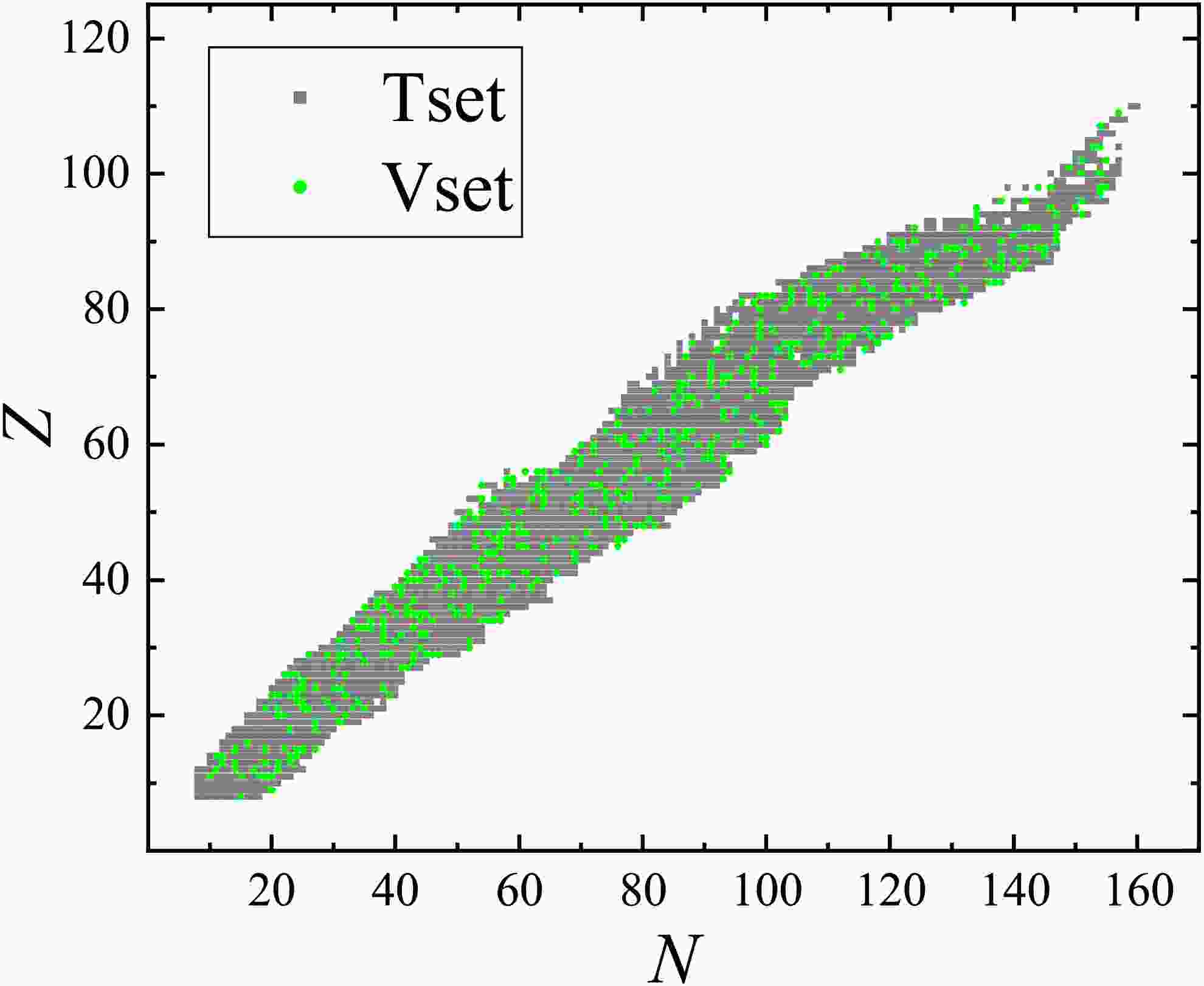
and $ a_{\upsilon} $, $ k_{\upsilon} $, $ a_{\rm{s}} $, $ k_{\rm{s}} $, $ a_{\rm{c}} $, $ f_{\rm{p}} $, $ {d_{{\rm{n}}}} $, $ {d_{{\rm{p}}}} $, and $ {d_{{\rm{np}}}} $ are adjustable parameters. The optimized parameters (in MeV) obtained by least squares fitting are $ a_{\upsilon}=15.628 $, $ k_{\upsilon}=1.860 $, $ a_{\rm{s}}= -17.881 $, $ k_{\rm{s}}=2.292 $, $ a_{\rm{c}}=-0.711 $, $ f_{\rm{p}}=1.120 $, $ {d_{{\rm{n}}}}=-4.873 $, $ {d_{{\rm{p}}}}=-5.102 $, and $ {d_{{\rm{np}}}}=7.188 $, and the root mean square deviation (RMSD) is 2.543 MeV for describing the experimental binding energies compiled in the AME2020 database [9].

For the first numerical experiment based on the AME2020 database [9], nuclei with experimental binding energies compiled in the AME2020 and $ N, Z \geq 8 $ are randomly split into a training set (80%) and a validation set (20%), and their positions on the nuclide chart are presented in Fig. 1, labeled by gray squares and green circles, respectively. The deviations between the experimental and corresponding theoretical binding energies calculated with the LDM (see Eq. (7)) for the nuclei in the training set are adopted as the training targets y defined in Eq. (6).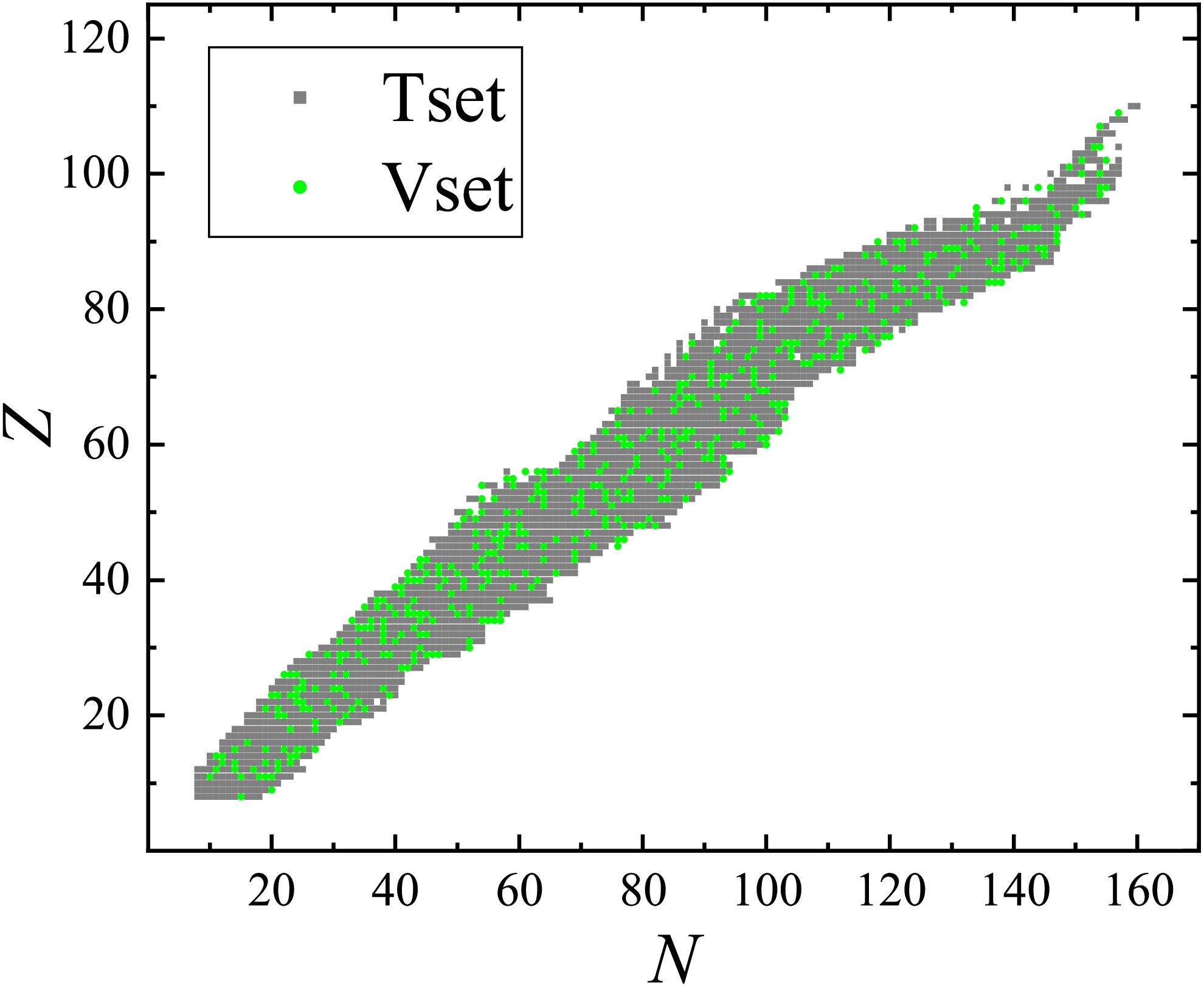

Figure 1.  (color online) Positions of nuclei in the training set (gray squares) and validation set (green circles)

As shown in the third column of Table 1, the RMSD of the training (validation) set decreased from 2.571 (2.425) to 0.241 (0.384) MeV after applying the BNN, with a considerable improvement of 90.6% (84.2%).Figure 2 displays the experimental-theoretical binding energy deviations $ \Delta E$ for the LDM, with the black squares and red circles corresponding to the results without and with the BNN optimization, respectively. The BNN was effective in optimizing the LDM predictions, particularly for nuclei near shells, and the RMSD of the binding energies for nuclei in both the training and validation sets decreased from 2.543 to 0.304 MeV.

	Models	LDM	FRDM [14]	WS4 [18]	HFB31 [23]	RMF [26]	DZ [19]	GK+J [33, 54, 55]
Training set	$ \sigma_{\rm{pre}} $	2.571	0.607	0.297	0.600	2.101	0.433	0.809
	$ \sigma_{\rm{post}} $	0.241	0.231	0.252	0.332	0.328	0.341	0.458
	$ \Delta \sigma $	90.6	61.9	15.1	44.6	84.3	21.2	43.3
Validation set	$ \sigma_{\rm{pre}} $	2.425	0.601	0.283	0.532	2.095	0.405	0.891
	$ \sigma_{\rm{post}} $	0.384	0.369	0.275	0.408	0.531	0.387	0.603
	$ \Delta \sigma $	84.2	38.6	2.8	23.3	74.6	4.4	32.3

Table 1.  RMSDs (in MeV) and relative improvements $ \Delta \sigma $ (in %) of theoretical nuclear mass (or binding energy) predictions for different models in comparison with the experimental data compiled in the AME2020 database [9]. Rows $ 2- 4 $ ($ 5- 7 $) represent the results of the training (validation) set. $ \sigma_{\rm{pre}} $ and $ \sigma_{\rm{post}} $ correspond to the RMSD values before and after applying the BNN, respectively.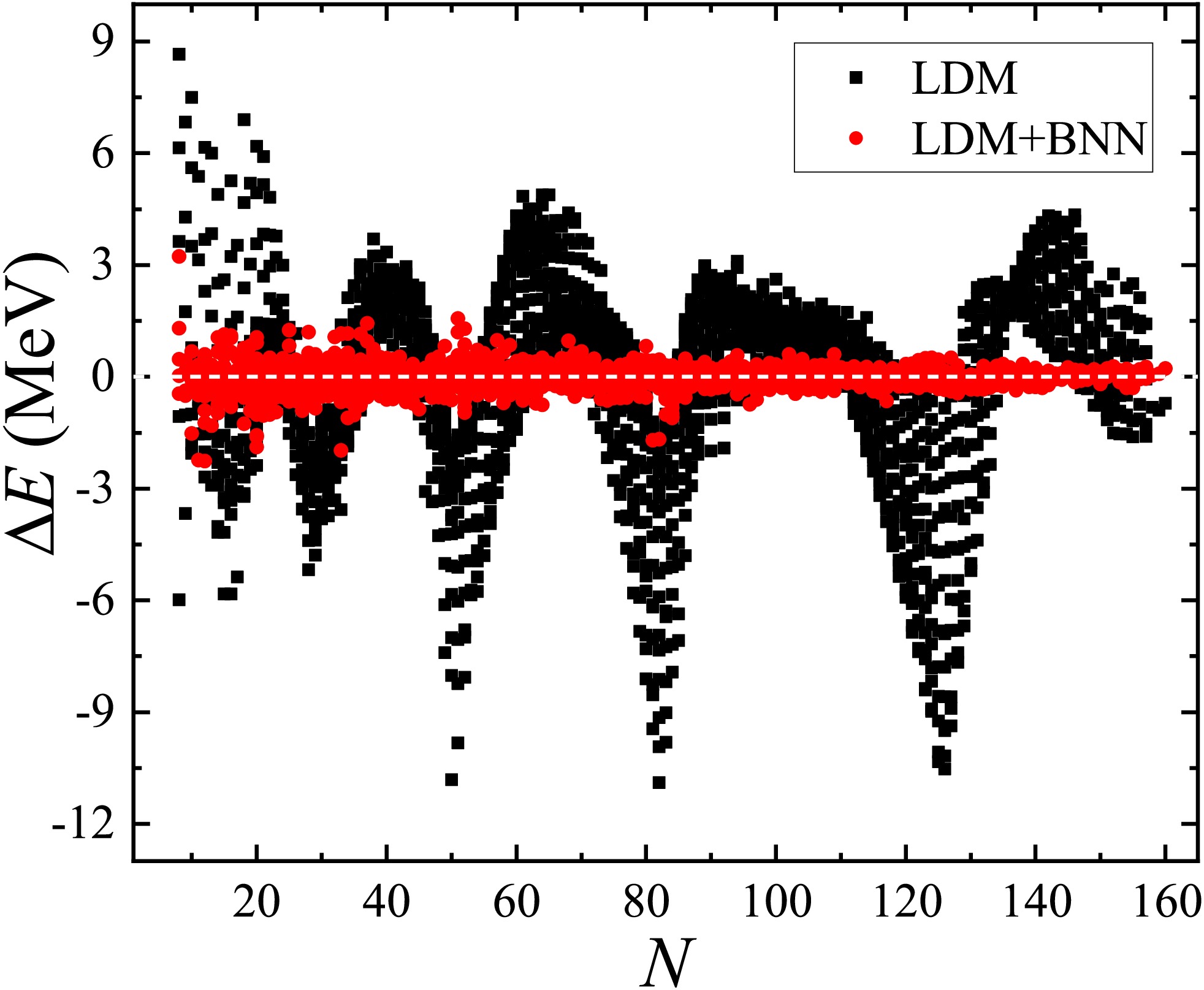

Figure 2.  (color online) Original (labeled by black squares) and BNN optimized (labeled by red circles) experimental-theoretical binding energy deviations $\Delta E $ (in MeV) for the LDM

The second numerical experiment involving the evaluation of the extrapolation from the AME2012 [39] to the AME2020 database [9] was similar to the first one, except that nuclei with $ N, Z \geq 8 $ and experimental binding energies compiled in the AME2012 were assigned to the training set, whereas those with new measurements in the AME2020 (absent from the AME2012) were assigned to the validation set. The RMSD of the training set decreased from 2.532 to 0.251 MeV, and that of the validation set decreased from 2.696 to 0.647 MeV, as shown in the third row of Table 2. The relative improvements were 90.1% and 76.0%, respectively. The BNN optimized the LDM successfully for the extrapolations of nuclear binding energies.

Models	Training set				Validation set
	$ \sigma_{\rm{pre}} $	$ \sigma_{\rm{post}} $	$ \Delta \sigma $		$ \sigma_{\rm{pre}} $	$ \sigma_{\rm{post}} $	$ \Delta \sigma $
LDM	2.532	0.251	90.1		2.696	0.647	76.0
FRDM [14]	0.579	0.235	59.4		0.963	0.508	47.2
WS4 [18]	0.298	0.263	11.7		0.364	0.340	6.6
HFB31 [23]	0.570	0.319	44.0		0.910	0.744	18.2
RMF [26]	2.042	0.378	81.5		3.144	1.039	66.9
DZ [19]	0.394	0.329	16.5		0.836	0.791	5.4
GK+J [33, 54, 55]	0.786	0.509	35.2		1.427	1.010	29.2

Table 2.  RMSDs (in MeV) and relative improvements $ \Delta \sigma $ (in %) for the extrapolations of nuclear masses (or binding energies) from the AME2012 [39] to the AME2020 database [9]. Columns $ 2 - 4 $ ($ 5 - 7 $) represent the results of the training (validation) set. $ \sigma_{\rm{pre}} $ and $ \sigma_{\rm{post}} $ correspond to the RMSD values before and after applying the BNN, respectively.

Similar to the first numerical experiment in Sec. III.A, the BNN was also employed to optimize other models based on the AME2020 database [9], and the results are listed in the columns $ 4 - 9 $ of Table 1 for comparison. The accuracy of these models improved on both the training and validation sets, particularly for the LDM, FRDM [14], and RMF [26]. We note that the GK+J [33, 54, 55] in the last column also showed considerable improvements of 43.3% and 32.3% for the training and validation sets, respectively. In contrast to the other global models, the GK+J is constructed based on the assumption of linear interactions between neighboring nuclei. Therefore, the BNN is also applicable to this type of local models.

As examples, the experimental-theoretical deviations of the nuclei in both the training and validation sets for the LDM and RMF [26] are presented in Fig. 3. Panels (a) and (b) present the deviations without and with the BNN optimization for the RMF, respectively, and panels (c) and (d) present those for the LDM. Large deviations are observed in panels (a) and (c), particularly for nuclei near shells and with $ N \sim 80-140 $, $ Z \sim 70-100 $ for the RMF, which may arise from missing physics in these models. In contrast, the deviations in panels (b) and (d) show significant reductions with the BNN optimizations, and most of them are less than 250 keV.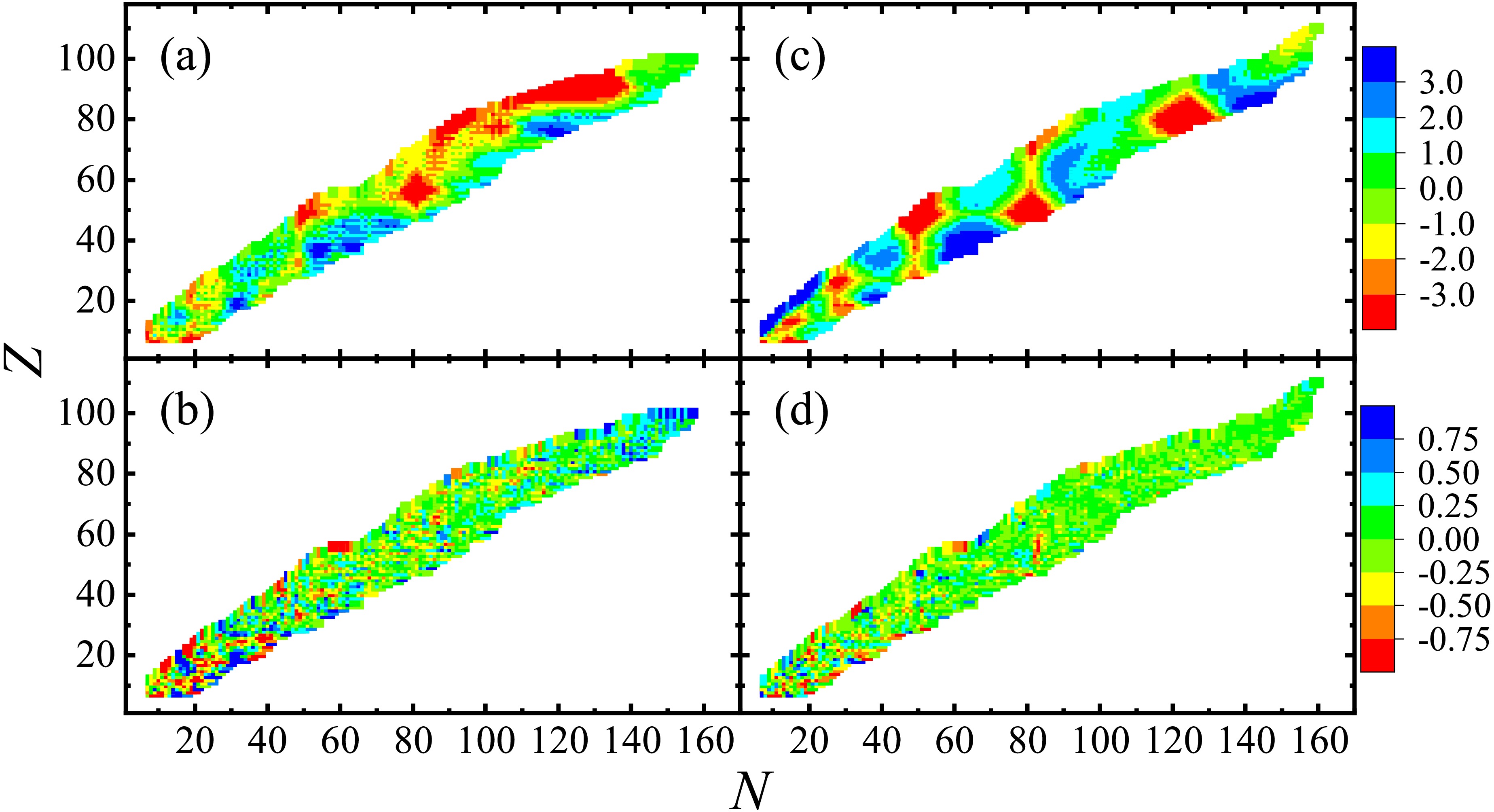

Figure 3.  (color online) Experimental-theoretical deviations (in MeV) of nuclei in both the training and validation sets, based on the AME2020 database [9]. Panels (a) [(c)] and (b) [(d)] present the original and BNN optimized deviations for the RMF [26] (LDM), respectively.

Table 2 summarizes the RMSDs of extrapolations from the AME2012 [39] to the AME2020 [9] for different models, before and after applying the BNN. The accuracy of both the training and validation sets for these models improved with the BNN optimizations. Considering the LDM, FRDM [14], and RMF [26] as examples, the experimental-theoretical deviations for the validation sets are presented in panels (a), (b), and (c) of Fig. 4, respectively. The black squares and red circles correspond to deviations without and with the BNN optimizations, respectively, and their error bars correspond to the theoretical uncertainties and experimental errors of these nuclear masses in the validation sets. The BNN is also appropriate for the extrapolations of nuclear masses (or binding energies) for both global and local models. Compared with the first type of numerical experiment (see Table 1), although the RMSDs of the validation sets for these global models were significantly larger in extrapolations, the relative improvements $ \Delta \sigma $ did not change significantly.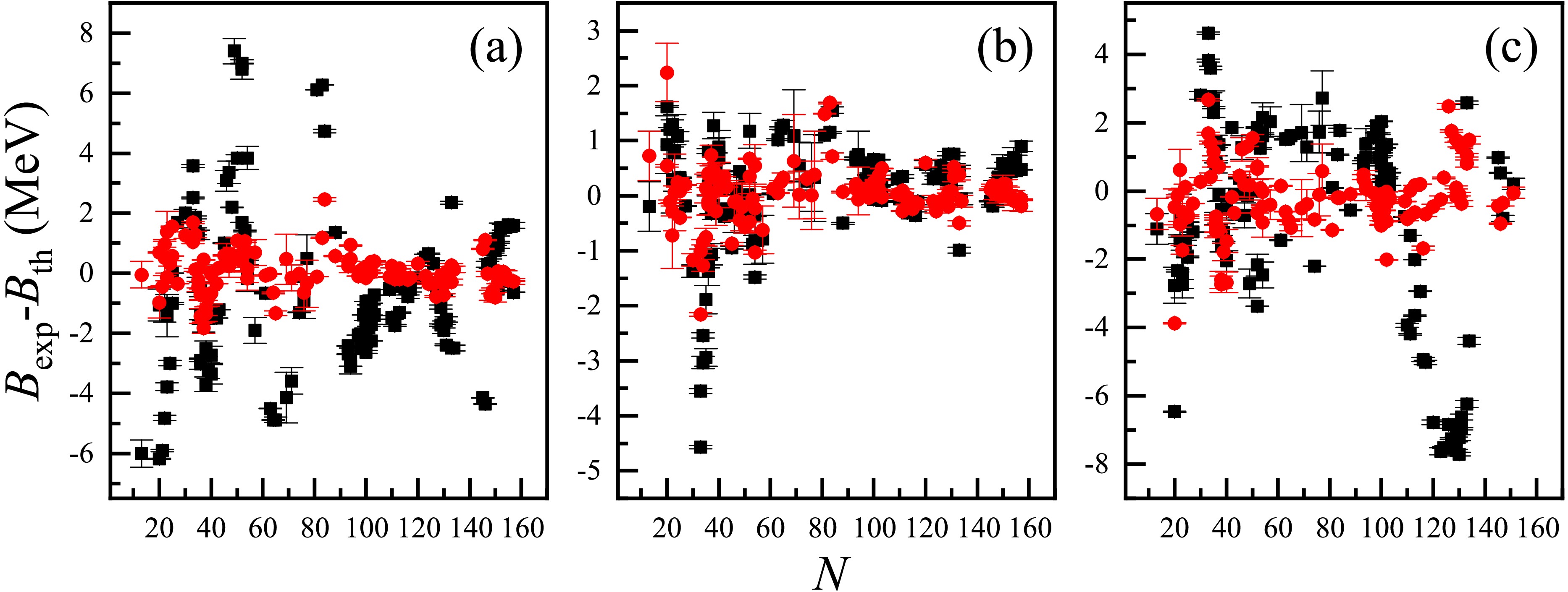

Figure 4.  (color online) Experimental-theoretical deviations (in MeV) of the extrapolations from the AME2012 [39] to the AME2020 [9], for nuclei in the validation sets. Panels (a), (b), and (c) correspond to the results of the LDM, FRDM [14], and RMF [26], respectively. The black squares and red circles represent the original and BNN optimized deviations, respectively, and their error bars correspond to the theoretical uncertainties and experimental errors of these nuclear masses.

Considering the favorable optimizations of both the training and validation sets discussed in Sec. III.B, the BNN was applied to these models based on the AME2020 [9], i.e., nuclei with $ N, Z \geq 8 $ and experimental values from the AME2020 [9] were assigned to a training set. The distance from the β-stability line ε was defined as $ Z_{0}-Z $ [41, 49, 57, 58], where $ Z_{0} $ is the integer closest to $ A/(1.98+ 0.0155A^{2/3}) $, and $ \varepsilon > 0 $ ($ \varepsilon < 0 $) represents neutron-rich (neutron-deficient) nuclei. Figure 5 presents the RMSDs of the FRDM [14], LDM, and RMF [26] versus ε, with the black squares and red circles corresponding to the cases without and with the BNN applied, respectively. The RMSDs for these models decreased after the BNN optimization, and most of them were less than 0.5 MeV. In addition, the original fluctuation of RMSDs as $ |\varepsilon| $ increased was significantly reduced when the BNN was applied, further reflecting the reliability of the BNN in extrapolations.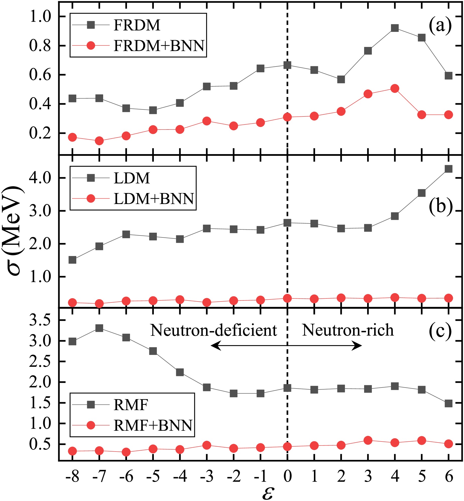

Figure 5.  (color online) RMSDs between the theoretical nuclear masses (or binding energies) and the experimental data obtained from the AME2020 database [9] versus ε (the distance from the β-stability line). Panels (a), (b), and (c) respectively correspond to the results of the FRDM [14], LDM [13], and RMF [26]. The black squares and red circles represent the RMSDs without and with the BNN applied, respectively.

Accordingly, single-neutron separation energies $ S_{\rm{n}} $ were calculated using the difference of binding energies for neighboring nuclei. Considering the S, Sb, and Fm isotopes ($ Z=16, 51 $, and 100) for example, panels (a), (b), and (c) of Fig. 6 present their $ S_{\rm{n}} $ versus the neutron number N. The results for the FRDM [14], LDM [13], and RMF [26] with the BNN optimized are indicated by the black circles, blue upper triangles, and green lower triangles, respectively. The experimental values obtained from the AME2020 database [9] (indicated by red stars) are also given for comparison. The theoretical $ S_{\rm{n}} $ values of these models after the BNN was applied were consistent with the experimental values, and the odd-even staggerings of $ S_{\rm{n}} $ were well reproduced.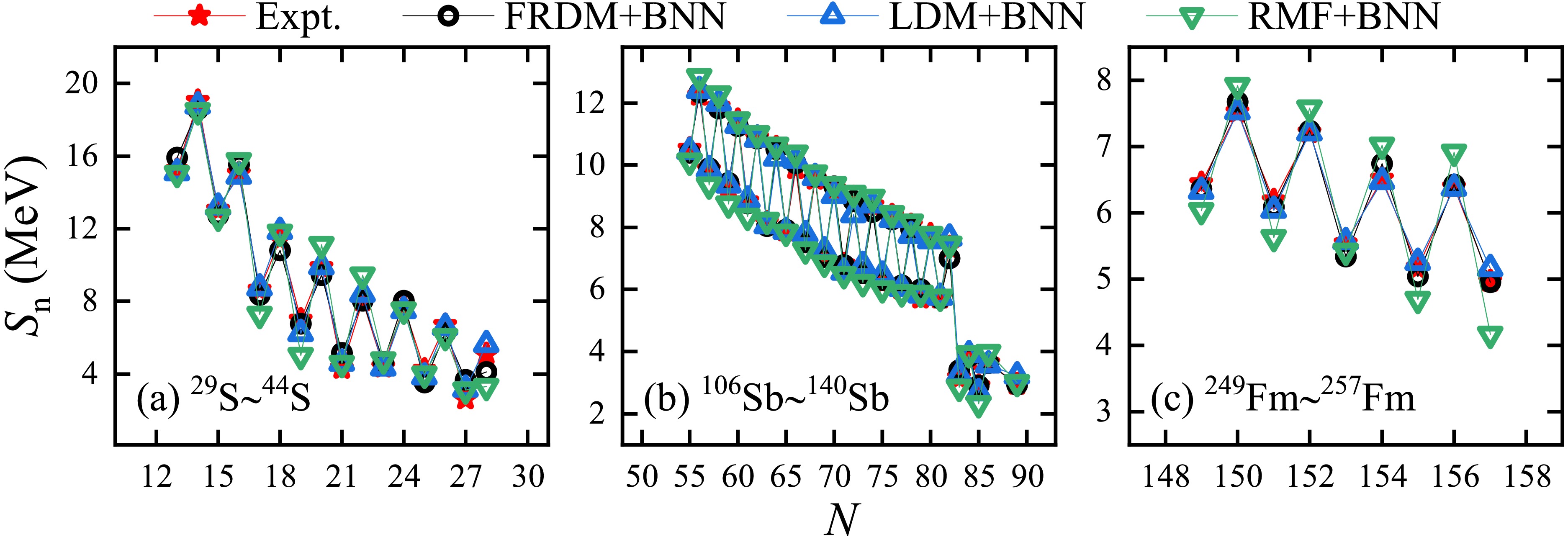

Figure 6.  (color online) Single-neutron separation energies S_n versus the neutron number N. Panels (a), (b), and (c) correspond to the S, Sb, and Fm isotopes, respectively. The theoretical results of the FRDM [14], LDM, and RMF [26] with the BNN optimized are indicated by the black circles, blue upper triangles, and green lower triangles, respectively. The red stars represent the experimental data obtained from the AME2020 database [9].

In this study, a BNN was applied to improve the accuracy of describing and predicting masses (or binding energies) of nuclei with $ N, Z \geq 8 $ for theoretical models, including the LDM [55], DZ [19], FRDM [14], WS4 [18], HFB31 [23], RMF [26], and GK+J [33, 54, 55]. Two types of numerical experiments were considered. One was based on the AME2020 database [9], where 80% (20%) nuclei with experimental masses were assigned to the training (validation) set. The other corresponded to an extrapolation, where the training set contained nuclei with experimental masses compiled in the AME2012 [39] and the validation set contained nuclei with newly measured masses in the AME2020 [9] that were not included in the AME2012.

The BNN proved to be effective, as the RMSDs of both the training and validation sets decreased in these numerical experiments, not only for global models but also for the local model GK+J. In particular, the RMSDs were reduced by 81.5%−90.6% (66.9%−84.2%) for the training (validation) sets of the LDM and RMF [26]. Note that the RMSDs of the validation sets were significantly larger in extrapolations compared with the first numerical experiment, whereas the relative improvements did not change significantly. The reliability of the BNN in extrapolations was also discussed based on the AME2020 [9]. Most RMSDs with $ -8 \leq \varepsilon \leq 6 $ were reduced to below 0.5 MeV after applying the BNN. The single-neutron separation energies of the S, Sb, and Fm isotopes, calculated using the BNN-optimized predicted nuclear masses of these theoretical models, showed good agreement with the experimental values, which also confirmed the reliability of the BNN.