


 Abstract
 HTML
HTML Reference
 Related
 PDF
PDF


-
Fission in heavy and superheavy elements can occur either spontaneously or be induced by various particles and photons. Neutron-induced fission has been extensively studied due to its role in nuclear energy generation [1−4]. Proton-induced fission has also been well-documented by Deppman, Ayyad, and Gikal et al. [5−7]. Additionally, heavy energetic nuclei can induce fission through fusion-fission reactions, as demonstrated in various studies [8−11]. Photon-induced fission is another significant type of fission, with contributions from several researchers [12−14].
Since the discovery of fission and its application in nuclear energy production in the late 1940s, nuclear scientists have primarily focused on studying binary fission. However, the ternary fission in which a heavy nucleus splits into three fragments emerged as an intriguing source of high-energy alpha particles. This rare type of nuclear reaction was first identified by Chinese and French scientists, including San-Tsiang, Chastel, and Zah-Wei [15−19]. Cold ternary fission refers to the disintegration of an unstable heavy or superheavy nucleus into three fission fragments, neglecting neutrons and other types of radiation [20−31]. This process effectively reveals the behavior of nuclear systems at the scission point.
True ternary fission, where the parent nucleus splits into three fragments with comparable masses, is a rare phenomenon observed in the decay of certain heavy and superheavy nuclei with high fissility parameters [32, 33]. Although this type of ternary fission has been extensively studied [34−42], its theoretical characteristics are not fully understood yet. True ternary fission typically occurs in heavy nuclei with high fissility parameter (
$Z^2/A > 31$ ) [32].According to
$ \check{a} $ Sndulescu et al. [43, 44], cold ternary fission is similar to cluster radioactivity [45, 46], representing a low energy rearrangement of nucleons from the ground state of the initial nucleus to the ground states of three final fragments. Delion et al. [47] provided a quantum description of the cold ternary fission of a$ {}^{252}\text{Cf} $ isotope within a stationary scattering formalism, calculating the preformation amplitude of$ ^4\text{He} $ and$ {}^{10}\text{Be} $ light-charged particles formed during the process [44, 48, 49]. Furthermore, they employed a double-folding potential and$ \text{M3Y} $ nucleon-nucleon forces to study the isotopic yields in the cold ternary fission of the$ {}^{248}\text{Cm} $ isotope, without including preformation factors.The recently proposed
$ \text{TCM} $ by Balasubramaniam and Manimaran [50] builds on the preformed cluster model ($ \text{PCM} $ ) introduced by Gupta et al. [51]. This approach has been widely applied to investigate the various aspects of ternary fission in isotopes of Californium ($ \text{Cf} $ ), Uranium ($ \text{U} $ ), Plutonium ($ \text{Pu} $ ), and Curium ($ \text{Cm} $ ) [52−57].The competition between binary and ternary fission with α-decay in heavy and superheavy isotopes has garnered considerable theoretical and experimental interest [46, 47]. A three-body equatorial model was introduced to examine the cold ternary fission of the
$ ^{252}\text{Cf} $ isotope, accompanied by α-particles, using an approach including double-folding nuclear potential [43]. Rosen and Hudson [21] provided experimental evidence that the probability of true ternary fission is significantly lower than that of binary fission (approximately$ 6.7 \pm 3 $ per$ 10^6 $ symmetric binary fissions) in the thermal-neutron-induced fission of$ ^{235}\text{U} $ . Green and Livesey [58, 59] utilized photographic plate techniques to measure particle emissions during fission, finding that approximately 1% of events involved emission of light particles, such as α.Farwell, Segre, and Wiegand conducted detailed studies using the coincidence counting method to determine the frequency of long-range charged particle emission during fission, predominantly α. Manimaran and Balasubramaniam [52, 53] investigated the influence of deformation and orientation on cold α-particles and
$ {}^{10}\text{B} $ -accompanied ternary fission of the$ ^{252}\text{Cf} $ isotope. They applied the liquid-drop formalism combined with the Yukawa-plus-exponential nuclear potential and nuclear shape parametrization to determine the ternary-to-binary fission probability ratio using equatorial geometry [60].Recent observations have identified various isotopes of
$ \text{He} $ ,$ \text{Li} $ ,$ \text{Be} $ , B, and C as light charged particles ($ \text{LCPs} $ ) in the spontaneous ternary fission of$ {}^{252}\text{Cf} $ [54, 55].Building on our previous studies [61, 62], which examined the ternary fission of
$ ^{248}\text{Cf} $ accompanied by$ ^{4}\text{He} $ ,$ ^{10}\text{Be} $ ,$ ^{14}\text{C} $ ,$ ^{14}\text{N} $ , and$ ^{16}\text{O} $ in equatorial geometry and compared the results in equatorial and collinear geometries for the ternary fission of the$ ^{244}\text{Fm} $ isotope accompanied by$ ^{8}\text{Be} $ ,$ ^{28}\text{Si} $ ,$ ^{58}\text{Ni} $ , and$ ^{90}\text{Zr} $ , this study explored fission dynamics. Specifically, it compared the equatorial and collinear geometries, focusing on accompanying heavy fragments with comparable masses in the true ternary fission of the$ ^{248}\text{Cf} $ isotope.Synthesized superheavy isotopes have been an active area of research in nuclear physics [63]. The Californium nucleus was discovered and synthesized in 1950 at Lawrence Berkeley National Laboratory (
$ \text{LBNL} $ ) by bombarding a Curium nucleus with α-particles. This nucleus has 20 known isotopes, most synthesized through successive neutron bombardment and β-decay. The$ ^{248}\text{Cf} $ isotope is produced through$ \beta^{-} $ decay of the$ ^{248\ast}\text{Bk} $ isotope.The remainder of this paper is organized as follows. Section II describes the theoretical method used to calculate the ternary fission process, focusing on the employed approach. Section III presents the results and provides an in-depth discussion. Finally, Section IV concludes the paper and briefly summarizes the findings.
-
The ternary fission process closely resembles binary fission, differing primarily in the emission of
$ \text{LCPs} $ during the final stage of the scission process. The study of ternary fission provides insights not only into fission dynamics but also nuclear structure. Theoretical frameworks have been developed to track$ \text{LCP} $ trajectories, offering tools to analyze statistical and dynamical characteristics of fission, especially scission criteria [64, 65].The energy released in ternary fission (Q-value) is calculated as
$ Q = M - \sum\limits_{i = 1}^{3} m_{i}, $

(1) where M is the mass excess of the parent nucleus, and
$ m_i $ ($ i = 1, 2, 3 $ ) are the mass excess of three fragments in units of$ \text{MeV} $ [66]. A positive Q-value is required for fission to occur, which is shared as kinetic energies of the fragments.The interaction potential between fragments consists of the Coulomb and nuclear proximity potentials [67, 68]
$ V = \sum\limits_{i = 1}^{3} \sum\limits_{j>i} \left( V^{ij}_c + V^{ij}_p \right). $

(2) The Coulomb potential for interaction of spherical fragments is simply defined as
$ V^{ij}_c = \frac{Z_i Z_j e^2}{R_{ij}}, $

(3) where
$ Z_i $ and$ Z_j $ are atomic numbers, and$ R_{ij} $ is the center-to-center distance between interacting fragments. The effective radius$ R_x $ for each fragment is defined as$ R_x = 1.28A_x^{1/3} - 0.76 + 0.8A_x^{-1/3}, $

(4) where
$ A_x $ is the mass number of fragment x.The nuclear proximity potential
$ V_p(s) $ is defined as [69]$ V_p(s) = 4\pi \gamma R_\delta \Phi\left(\frac{s}{b}\right), $

(5) where
$ \Phi(\xi) $ depends on the separation$ s/b $ between fragments and is given by [70]$ \Phi(\xi) = \begin{cases} -\dfrac{1}{2}(\xi - 2.54)^2 - 0.0852(\xi - 2.54)^3, & \xi < 1.2511, \\ -3.437 \exp(-\xi/0.75), & \xi \geq 1.2511. \end{cases} $

(6) In the context of ternary fission, the dimensionless parameter
$ \xi = \dfrac{s}{b} $ represents the scaled distance between interacting fragments. For simplicity, it is often assumed that one of three fragments remains fixed during analysis.Geometrical configurations of fragments are key to understanding penetration probabilities and fission half-lives. Typically, two types of geometrical configurations of fragments are considered:
● Collinear: Fragments align along a straight line joining the centers of three fragments.
● Equatorial: The fixed
$ LCP $ is ejected perpendicularly to the separation line of the other two fragments.These geometrical arrangements of fragments significantly influence the energy distribution among the fragments, their angular momentum, and neutron emission characteristics. In the collinear configuration, the fragments move along a straight line connecting their centers. In contrast, the equatorial configuration involves fixed light fragment being ejected perpendicular to the line connecting the centers of the other two fragments. Fig. 1 illustrates the tripartition of fragments in both the equatorial and collinear geometries, with a separation distance
$ s > 0 $ indicating a moment after separation of fragments.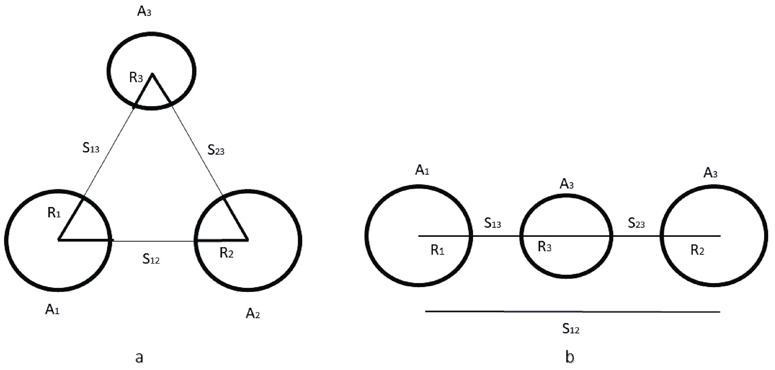
Figure 1. Schematic diagram of fragment geometries for ternary fission: equatorial (a) and collinear (b) arrangement of fragments a moment after separation of fragments in output channel (
$s > 0$ ).In the equatorial configuration, a symmetric separation is often assumed for simplicity. Also, it is considered that the fragments disperse with identical speeds and equal separation distances (
$ s = s_{12} = s_{13} = s_{23} $ ). However, this assumption does not account for differences in fragment velocities caused by repulsive Coulomb forces, particularly affecting the lightest fragment ($ A_3 $ , also referred to as the$ \text{LCP} $ , which moves faster than the heavier ones due to conservation of energy). To address this discrepancy, an initial relationship$ k \times s_{12} = s_{13} = s_{23} $ can be considered, where k varies within the interval$ 0 < k < 1 $ [50]. Notably, studies indicate that trends in relative yields and fragmentation potential barriers remain largely unaffected by the choice of$ k<1 $ . Therefore, the assumption of$ k = 1 $ does not considerably affect the final results.The parameter S further describes the fragment geometry:
$ S = 0 $ represents a touching configuration,$ S < 0 $ denotes overlapping fragments, and$ S > 0 $ indicates separated fragments configurations. In the collinear geometry, with$ A_3 $ positioned between the other two fragments, the distance between the surfaces of fragments 1 and 3, or 2 and 3, is denoted by$ s = s_{13} = s_{23} $ . The center-to-center distance between fragments 1 and 2 is then given as$ s_{12} = 2(R_3 + s). $

(7) The penetration probability P is calculated using the
$ \text{WKB} $ approximation:$ P = \exp\left(-\frac{2}{\hbar} \int_{S_{\text{in}}}^{S_{\text{out}}} \sqrt{2\mu(V - Q)} \, {\rm d} S\right), $

(8) where
$ S_{\text{in}} $ and$ S_{\text{out}} $ are the inner and the outer turning points, respectively, and μ is the reduced mass of three fragments obtained using$ \mu = m \frac{A_1 A_2 A_3}{A_1 A_2 + A_1 A_3 + A_2 A_3}. $

(9) The half-life of ternary fission is evaluated using
$ T_{1/2} = \frac{\ln 2}{\lambda}, \quad \lambda = \nu P, $

(10) where ν is the assault frequency, which is simply obtained by the following relation [50]:
$ \nu = \frac{\omega}{2\pi} = \frac{2E_\nu}{h}. $

(11) The vibrational energy
$ E_\nu $ is then obtained as follows:$ E_\nu = Q \left[0.056 + 0.039\exp\left(\frac{4 - A_{\text{LCP}}}{2.5}\right)\right] \, \text{MeV}. $

(12) Finally, the relative yield
$ Y(A_i, Z_i) $ for each fragmentation with a given geometry is determined by$ Y(A_i, Z_i) = \frac{P(A_i, Z_i)}{\sum P(A_i, Z_i)}. $

(13) The resultant relative yields are used to evaluate the decay constant and relative half-life.
It is also important to check the neutron emission in the ternary fission process, which is considered in this research to compare the obtained results with the no neutron emission case of each selected combination.
-
In this study, the ternary fission of the
$ ^{248}\text{Cf} $ isotope was analyzed, focusing on fragment combinations and their geometries. For collinear geometries, we systematically examined the driving potential (V) for each fragment configuration, where$ A_1 $ ,$ A_2 $ , or$ A_3 $ occupy the middle position in the fragment moving line. Reaction Q-value, penetration probability (${P}$ ), and decay constant were evaluated for each combination constructed at given geometry for one neutron emission and no neutron emission to highlight the influence of fragment placement and neutron emission. Among 128 unique sets of$ Z_1 $ ,$ Z_2 $ , and$ Z_3 $ combinations, 40 sets of them with higher penetration probabilities were selected, as tabulated in Table 1. The relationship between the Q-value and atomic numbers$Z_1$ ,$Z_2$ , and$Z_3$ is depicted in Fig. 2.Combination Q
/MeV${\boldsymbol{V} } _{e}$ 

/MeV${\boldsymbol{V} } _{A3}$ 

/MeV${\boldsymbol{V} } _{A2}$ 

/MeV${\boldsymbol{V} } _{A1}$ 

/MeV${\boldsymbol{P} } _{e}$ 

${\boldsymbol{P} } _{A3}$ 

${\boldsymbol{P} } _{A2}$ 

${\boldsymbol{P} } _{A1}$ 

ν $ \times 10^{21} $ 

$ \lambda_{\text{e}} $ 

$ \lambda_{\text{A3}} $ 

$ \lambda_{\text{A2}} $ 

$ \lambda_{\text{A1}} $ 

$ ^{50} {\rm{Ca}}$ +

$ ^{64} {\rm{Fe}}$ +

$ ^{134} {\rm{Te}}$ 

244.33 75.40 24.48 4.05 1.24 6.74e-51 2.31e-31 1.41e-21 5.13e-16 6.62 4.5e-29 1.5e-09 9.4e+00 3.4e+06 $ ^{48} {\rm{Ca}}$ +

$ ^{68} {\rm{Ni}}$ +

$ ^{132} {\rm{Sn}}$ 

251.47 75.46 21.12 5.02 0.01 1.63e-49 4.11e-29 2.17e-21 8.37e-15 6.81 1.1e-27 2.8e-07 1.5e+01 5.7e+07 $ ^{48} {\rm{Ca}}$ +

$ ^{67} {\rm{Co}}$ +

$ ^{133} {\rm{Sb}}$ 

245.71 77.92 25.23 6.44 3.73 1.59e-51 2.12e-31 1.98e-22 1.04e-16 6.65 1.1e-29 1.4e-09 1.3e+00 6.9e+05 $ ^{54} {\rm{Ti}}$ +

$ ^{60} {\rm{Cr}}$ +

$ ^{134} {\rm{Te}}$ 

242.42 78.73 27.14 2.67 8.44 5.31e-53 6.32e-33 3.82e-21 1.54e-19 6.57 3.5e-31 4.1e-11 2.5e+01 1.0e+03 $ ^{51} {\rm{Sc}}$ +

$ ^{64} {\rm{Fe}}$ +

$ ^{133} {\rm{Sb}}$ 

244.38 80.14 27.01 6.83 7.04 3.91e-53 1.43e-32 8.96e-23 1.55e-18 6.62 2.6e-31 9.4e-11 5.9e-01 1.0e+04 $ ^{53} {\rm{Sc}}$ +

$ ^{61} {\rm{Mn}}$ +

$ ^{134} {\rm{Te}}$ 

240.28 80.28 28.96 7.10 7.35 4.39e-54 5.80e-34 3.37e-23 3.53e-19 6.51 2.9e-32 3.8e-12 2.2e-01 2.3e+03 $ ^{54} {\rm{Ti}}$ +

$ ^{62} {\rm{Fe}}$ +

$ ^{132} {\rm{Sn}}$ 

248.41 80.42 25.16 6.43 7.11 7.66e-53 1.49e-31 2.68e-22 1.61e-18 6.73 5.2e-31 1.0e-09 1.8e+00 1.1e+04 $ ^{48} {\rm{Ca}}$ +

$ ^{76} {\rm{Zn}}$ +

$ ^{124} {\rm{Cd}}$ 

250.47 80.61 24.78 10.09 3.54 6.09e-53 2.75e-31 2.46e-24 1.06e-16 6.78 4.1e-31 1.9e-09 1.7e-02 7.2e+05 $ ^{48} {\rm{Ca}}$ +

$ ^{73} {\rm{Cu}}$ +

$ ^{127} {\rm{In}}$ 

247.33 81.49 26.68 10.60 5.29 1.36e-53 2.78e-32 1.38e-24 1.53e-17 6.70 9.1e-32 1.9e-10 9.3e-03 1.0e+05 $ ^{54} {\rm{Ti}}$ +

$ ^{61} {\rm{Mn}}$ +

$ ^{133} {\rm{Sb}}$ 

243.65 81.50 28.06 6.46 9.63 4.10e-54 2.86e-33 1.13e-22 5.65e-20 6.60 2.7e-32 1.9e-11 7.5e-01 3.7e+02 $ ^{51} {\rm{Sc}}$ +

$ ^{65} {\rm{Co}}$ +

$ ^{132} {\rm{Sn}}$ 

246.22 81.80 26.93 9.52 7.34 1.28e-53 2.11e-32 9.20e-24 1.55e-18 6.67 8.5e-32 1.4e-10 6.1e-02 1.0e+04 $ ^{48} {\rm{Ca}}$ +

$ ^{82} {\rm{Ge}}$ +

$ ^{118} {\rm{Pd}}$ 

252.27 82.63 24.86 12.97 4.09 5.01e-54 2.30e-31 8.51e-26 5.46e-17 6.83 3.4e-32 1.6e-09 5.8e-04 3.7e+05 $ ^{57} {\rm{V}}$ +

$ ^{58} {\rm{Cr}}$ +

$ ^{133} {\rm{Sb}}$ 

242.59 82.89 29.30 6.26 12.40 4.84e-55 5.33e-34 1.39e-22 2.02e-21 6.57 3.2e-33 3.5e-12 9.1e-01 1.3e+01 $ ^{56} {\rm{Cr}}$ +

$ ^{60} {\rm{Cr}}$ +

$ ^{132} {\rm{Sn}}$ 

245.98 83.64 28.03 4.16 15.44 8.65e-55 4.13e-33 1.56e-21 2.54e-22 6.66 5.7e-33 2.7e-11 1.0e+01 1.7e+00 $ ^{51} {\rm{Sc}}$ +

$ ^{68} {\rm{Ni}}$ +

$ ^{129} {\rm{In}}$ 

246.79 83.78 27.80 11.78 8.32 7.26e-55 5.55e-33 5.52e-25 4.20e-19 6.68 4.8e-33 3.7e-11 3.7e-03 2.8e+03 $ ^{50} {\rm{Ca}}$ +

$ ^{84} {\rm{Se}}$ +

$ ^{114} {\rm{Ru}}$ 

253.00 84.50 24.51 17.49 3.40 1.69e-55 1.37e-31 5.19e-28 4.66e-17 6.85 1.2e-33 9.4e-10 3.6e-06 3.2e+05 $ ^{48} {\rm{Ca}}$ +

$ ^{79} {\rm{Ga}}$ +

$ ^{121} {\rm{Ag}}$ 

248.41 84.69 27.87 14.57 6.84 1.97e-55 5.56e-33 1.27e-26 2.36e-18 6.73 1.3e-33 3.7e-11 8.5e-05 1.6e+04 $ ^{55} {\rm{V}}$ +

$ ^{61} {\rm{Mn}}$ +

$ ^{132} {\rm{Sn}}$ 

244.65 84.76 29.23 8.00 13.98 1.60e-55 8.96e-34 2.93e-23 8.90e-22 6.63 1.1e-33 5.9e-12 1.9e-01 5.9e+00 $ ^{80} {\rm{Ge}}$ +

$ ^{82} {\rm{Ge}}$ +

$ ^{86} {\rm{Se}}$ 

272.69 84.78 8.24 5.25 15.00 8.64e-56 2.43e-24 5.49e-23 2.75e-23 7.38 6.4e-34 1.8e-02 4.1e-01 2.0e-01 $ ^{55} {\rm{V}}$ +

$ ^{59} {\rm{V}}$ +

$ ^{134} {\rm{Te}}$ 

236.51 84.86 33.18 5.96 17.26 5.30e-57 2.31e-36 4.95e-23 7.89e-24 6.40 3.4e-35 1.5e-14 3.2e-01 5.1e-02 $ ^{50} {\rm{Ca}}$ +

$ ^{83} {\rm{As}}$ +

$ ^{115} {\rm{Rh}}$ 

250.73 85.21 26.68 17.00 4.71 3.25e-56 9.67e-33 5.00e-28 8.95e-18 6.79 2.2e-34 6.6e-11 3.4e-06 6.1e+04 $ ^{54} {\rm{Ti}}$ +

$ ^{68} {\rm{Ni}}$ +

$ ^{126} {\rm{Cd}}$ 

248.70 85.26 27.68 11.81 9.88 6.12e-56 3.59e-33 3.32e-25 4.10e-20 6.74 4.1e-34 2.4e-11 2.2e-03 2.8e+02 $ ^{78} {\rm{Zn}}$ +

$ ^{84} {\rm{Se}}$ +

$ ^{86} {\rm{Se}}$ 

271.17 85.66 9.39 10.23 11.92 1.93e-56 5.91e-25 3.16e-25 4.37e-22 7.34 1.4e-34 4.3e-03 2.3e-03 3.2e+00 $ ^{76} {\rm{Zn}}$ +

$ ^{82} {\rm{Ge}}$ +

$ ^{90} {\rm{Kr}}$ 

269.92 86.39 13.00 7.35 13.85 6.79e-57 1.31e-26 4.60e-24 7.02e-23 7.31 5.0e-35 9.6e-05 3.4e-02 5.1e-01 $ ^{50} {\rm{Ca}}$ +

$ ^{90} {\rm{Kr}}$ +

$ ^{108} $ Mo

252.54 86.77 25.10 20.88 4.96 6.19e-57 5.38e-32 8.07e-30 7.04e-18 6.84 4.2e-35 3.7e-10 5.5e-08 4.8e+04 $ ^{54} {\rm{Ti}}$ +

$ ^{82} {\rm{Ge}}$ +

$ ^{112} {\rm{Ru}}$ 

254.03 87.12 25.94 14.68 8.88 2.60e-57 1.53e-32 3.52e-27 6.76e-20 6.88 1.8e-35 1.0e-10 2.4e-05 4.6e+02 $ ^{79} {\rm{Ga}}$ +

$ ^{82} {\rm{Ge}}$ +

$ ^{87} {\rm{Br}}$ 

269.09 87.90 13.33 8.57 16.27 7.60e-58 8.26e-27 1.05e-24 4.01e-24 7.29 5.5e-36 6.0e-05 7.7e-03 2.9e-02 $ ^{80} {\rm{Ge}}$ +

$ ^{83} {\rm{As}}$ +

$ ^{85} {\rm{As}}$ 

269.63 88.00 9.50 10.37 18.16 8.23e-58 3.81e-25 1.99e-25 6.81e-25 7.30 6.0e-36 2.8e-03 1.5e-03 5.0e-03 $ ^{72} {\rm{Ni}}$ +

$ ^{86} {\rm{Se}}$ +

$ ^{90} {\rm{Kr}}$ 

266.93 88.17 15.30 12.65 12.57 4.03e-58 8.39e-28 1.35e-26 2.07e-22 7.23 2.9e-36 6.1e-06 9.7e-05 1.5e+00 $ ^{72} {\rm{Ni}}$ +

$ ^{82} {\rm{Ge}}$ +

$ ^{94} {\rm{Sr}}$ 

265.72 88.21 18.15 10.19 13.10 2.71e-58 3.66e-29 1.51e-25 1.04e-22 7.20 2.0e-36 2.6e-07 1.1e-03 7.5e-01 $ ^{78} {\rm{Zn}}$ +

$ ^{83} {\rm{As}}$ +

$ ^{87} {\rm{Br}}$ 

268.28 88.39 13.96 11.17 14.72 3.26e-58 3.76e-27 6.96e-26 1.57e-23 7.27 2.4e-36 2.7e-05 5.1e-04 1.1e-01 $ ^{79} {\rm{Ga}}$ +

$ ^{84} {\rm{Se}}$ +

$ ^{85} {\rm{As}}$ 

268.92 88.39 10.03 10.45 16.61 4.13e-58 1.96e-25 1.44e-25 2.72e-24 7.28 3.0e-36 1.4e-03 1.0e-03 2.0e-02 $ ^{76} {\rm{Zn}}$ +

$ ^{78} {\rm{Zn}}$ +

$ ^{94} {\rm{Sr}}$ 

265.87 88.66 18.34 7.05 16.88 1.43e-58 2.79e-29 3.81e-24 1.82e-24 7.20 1.0e-36 2.0e-07 2.7e-02 1.3e-02 $ ^{50} {\rm{Ca}}$ +

$ ^{94} {\rm{Sr}}$ +

$ ^{104} {\rm{Zr}}$ 

251.39 88.91 25.07 24.91 6.72 2.98e-58 3.79e-32 8.57e-32 9.20e-19 6.81 2.0e-36 2.6e-10 5.8e-10 6.3e+03 $ ^{75} {\rm{Cu}}$ +

$ ^{83} {\rm{As}}$ +

$ ^{90} {\rm{Kr}}$ 

266.34 89.47 16.30 12.62 14.89 5.77e-59 2.35e-28 1.27e-26 1.28e-23 7.21 4.2e-37 1.7e-06 9.2e-05 9.3e-02 $ ^{77} {\rm{Cu}}$ +

$ ^{85} {\rm{Br}}$ +

$ ^{86} {\rm{Se}}$ 

265.18 90.84 14.94 15.35 15.16 6.06e-60 7.19e-28 5.27e-28 5.49e-24 7.18 4.3e-38 5.2e-06 3.8e-06 3.9e-02 $ ^{72} {\rm{Ni}}$ +

$ ^{83} {\rm{As}}$ +

$ ^{93} {\rm{Rb}}$ 

263.75 90.95 19.08 14.57 15.51 5.90e-60 8.74e-30 1.32e-27 6.48e-24 7.14 4.2e-38 6.2e-08 9.4e-06 4.6e-02 $ ^{72} {\rm{Ni}}$ +

$ ^{87} {\rm{Br}}$ +

$ ^{89} {\rm{Br}}$ 

263.63 91.62 17.01 17.80 15.95 2.34e-60 7.22e-29 4.01e-29 3.82e-24 7.14 1.7e-38 5.2e-07 2.9e-07 2.7e-02 $ ^{66} {\rm{Fe}}$ +

$ ^{70} {\rm{Ni}}$ +

$ ^{112} {\rm{Ru}}$ 

252.15 92.45 29.65 13.45 18.48 2.66e-61 4.18e-35 5.19e-27 3.12e-25 6.83 1.8e-39 2.9e-13 3.6e-05 2.1e-03 $ ^{70} {\rm{Ni}}$ +

$ ^{81} {\rm{Ga}}$ +

$ ^{97} {\rm{Y}}$ 

260.20 92.92 23.90 13.17 19.22 2.51e-61 3.51e-32 3.16e-27 1.33e-25 7.05 1.8e-39 2.5e-10 2.2e-05 9.4e-04 Table 1. Calculated quantities of ternary fission for 248Cf isotope in different geometries and for selected combinations without neutron emission.
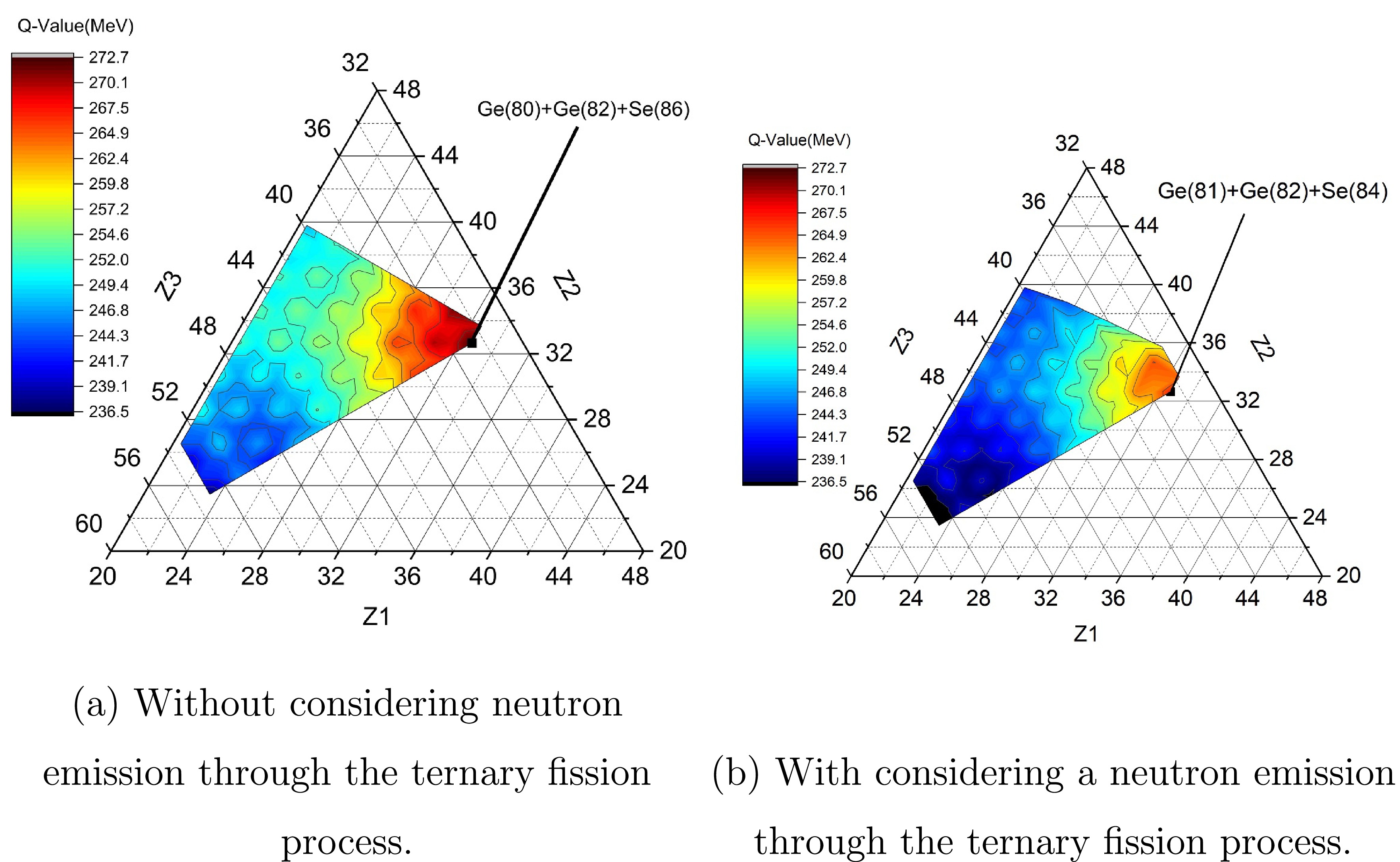
Figure 2. (color online) Q-Value for fragment atomic numbers
$Z_1$ ,$Z_2$ , and$Z_3$ for the ternary fission of 248Cf isotope.In the collinear configurations with
$ A_3 $ positioned in the middle of the two other fragments, the alignment of fragments reduced the Coulomb repulsion, resulting in lower driving potentials and higher penetration probabilities. For example, in the combination$ ^{80}\text{Ge} + ^{82}\text{Ge} + ^{86}\text{Se} $ , with a Q-value of 272.69 MeV,$ A_3 $ =$ ^{82}\text{Ge} $ provided significant stabilization due to magic neutron number$ (N = 50) $ . This combination, highlighted in Fig. 2, which shows the Q-value as a function of atomic numbers$ Z_1 $ ,$ Z_2 $ , and$ Z_3 $ , exhibited the highest Q-value among all configurations. The calculated driving potential$ (V_{cA3} = 8.23 \, \text{MeV}) $ facilitated a penetration probability of$ 2.43 \times 10^{-24} $ . The even-even nature of$ ^{80}\text{Ge} $ and$ ^{86}\text{Se} $ further enhanced the stability of this configuration. This case is also illustrated in Fig. 3(c), which presents the collinear geometry with$ A_3 $ in the middle.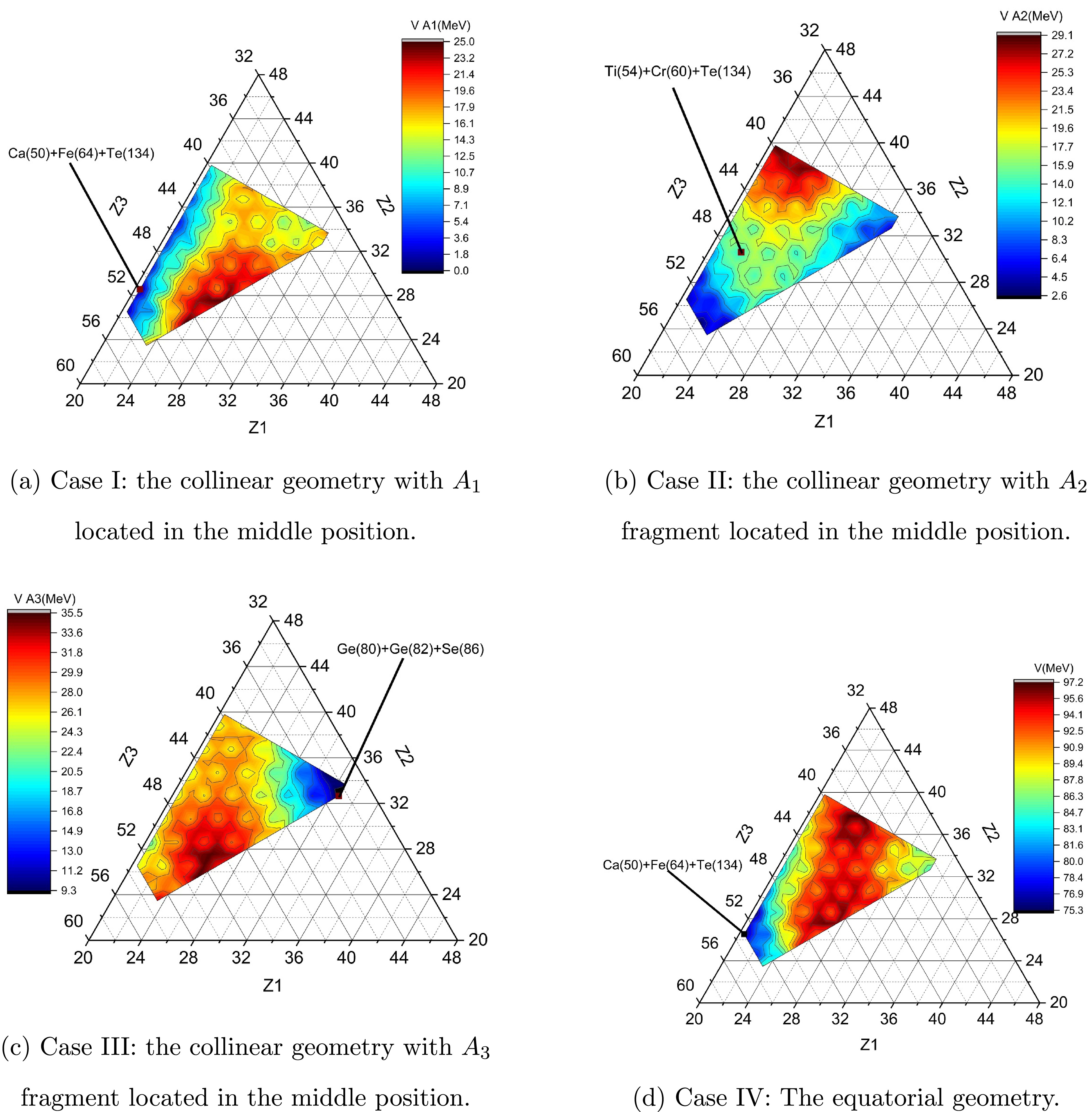
Figure 3. (color online) Driving potential for atomic numbers of the three fragments
$Z_1$ ,$Z_2$ , and$Z_3$ for various cases of ternary fission of 248Cf isotope.Similarly, for
$ ^{76}\text{Zn} + ^{82}\text{Ge} + ^{90}\text{Kr} $ ,$ A_3 $ =$ ^{82}\text{Ge} $ stabilizes the configuration through magic and near-magic properties of its constituent fragments. The driving potential$ (V_{cA3} = 13.00 \, \text{MeV}) $ is among the lowest observed, leading to a penetration probability of$ 1.31 \times 10^{-26} $ for this combination.When the lightest fragment
$ A_1 $ occupies the middle location, the driving potential decreases due to the lower Coulomb interaction between the other two heavier fragments positioned at the ends and lightest fragment occupying the middle. For instance, in the combination$ ^{48}\text{Ca} + ^{68}\text{Ni} + ^{132}\text{Sn} $ , where$ A_1 $ =$ ^{48}\text{Ca} $ is placed in the middle, the driving potential$ (V_{cA1} = 0.01 \, \text{MeV}) $ is relatively low. The resultant Q-value equal to 251.47$ \text{MeV} $ and penetration probability equal to$ 8.37 \times 10^{-15} $ are still favorable due to the double-magic nature of$ A_3 $ =$ ^{132}\text{Sn} $ and even-even near-magic configuration of$ A_2 $ =$ ^{68}\text{Ni} $ . This combination is illustrated in Fig. 3(a), where$ ^{132}\text{Sn} $ is highlighted due to its double-magic structure.In the combination
$ ^{50}\text{Ca} + ^{64}\text{Fe} + ^{134}\text{Te} $ , while$ A_1 $ =$ ^{50}\text{Ca} $ occupies the middle position, despite its stabilizing magic property$ (N = 50) $ , the overall driving potential$ (V_{cA1} = 1.24 \, \text{MeV}) $ remains very low due to the even-even nature of$ A_2 $ =$ ^{64}\text{Fe} $ and the magic nature$ N = 82 $ of$ A_3 $ =$ ^{134}\text{Te} $ . Consequently, the penetration probability$ (P = 5.13 \times 10^{-16}) $ is significantly high.When the intermediate-mass fragment
$ A_2 $ is placed in the middle, the driving potential is generally higher than in the combination when$ A_1 $ is located in the middle but lower than when$ A_3 $ occupies the middle position. For instance, in the$ ^{54}\text{Ti} + ^{60}\text{Cr} + ^{134}\text{Te} $ combination, when$ A_2 $ =$ ^{54}\text{Ti} $ is positioned in the middle, a driving potential of$ (V_{cA2} = 2.66 \, \text{MeV}) $ is achived, which is lower than this combination when magic fragment$ A_3 = ^{134}\text{Te} $ is located in the middle. The penetration probability$ (P = 3.82 \times 10^{-21}) $ remains favorable due to the stabilizing effects of$ A_1 = ^{54}\text{Ti} $ and$ A_3 $ =$ ^{134}\text{Te} $ , both of which are even-even nuclei, and one of them contains magic neutron number$ N = 82 $ . This configuration is highlighted in Fig. 3(b), where the minimum driving potential of combination$ ^{54}\text{Ti} + ^{60}\text{Cr} + ^{134}\text{Te} $ is emphasized.As stated in the previous section, we also studied one-neutron emission in the ternary fission process. To check the effects of one-neutron emission in the ternary fission process of the
$ ^{248} {\rm{Cf}}$ isotope, 10 combinations were selected for better comparison of their results with no neutron emission. The combinations have the same set of atomic numbers (Z), so the elements are the same, but their mass numbers are different. These combinations were chosen because they have the minimum driving potential and highest penetrating probability among all selected fragments combinations, both with and without considering neutron emission. As shown in Table 2, neutron emission reduces the Q-value of the fragments combination. This increase in the potential barrier leads to a lower penetration probability. As an example, for$ Z_1 = 20 $ ,$ Z_2 = 30 $ , and$ Z_3 = 38 $ , the favored combination is$ \mathrm{^{48}_{20}Ca} + \mathrm{^{76}_{30}Zn} + \mathrm{^{123}_{48}Cd} $ when considering neutron emission and$ \mathrm{^{48}_{20}Ca} + \mathrm{^{76}_{30}Zn} + \mathrm{^{124}_{48}Cd} $ without considering neutron emission. Their penetrating probabilities for$ A_1 $ located in the middle are$ 1.62 \times 10^{-20} $ and$ 1.06 \times 10^{-16} $ , respectively. This trend is observed in other geometries and combinations as well.Combination Q
/MeV${\boldsymbol{V} } _{A3}$ 

/MeV${\boldsymbol{V} } _{A2}$ 

/MeV${\boldsymbol{V} } _{A1}$ 

/MeV${\boldsymbol{V} } _{e}$ 

/MeV${\boldsymbol{P} } _{A3}$ 

${\boldsymbol{P} } _{A2}$ 

${\boldsymbol{P} } _{A1}$ 

${\boldsymbol{P} } _{e}$ 

Status $ ^{49} {\rm{Ca}}$ +

$ ^{64} {\rm{Fe}}$ +

$ ^{134} {\rm{Te}}$ 

237.97 31.66 11.15 7.20 82.84 6.35e-35 7.59e-25 1.50e-19 6.07e-55 Considering Neutron Emission $ ^{50} {\rm{Ca}}$ +

$ ^{64} {\rm{Fe}}$ +

$ ^{134} {\rm{Te}}$ 

244.33 24.48 4.05 1.24 75.40 2.31e-31 1.41e-21 5.13e-16 6.74e-51 Without Neutron Emission $ ^{48} {\rm{Ca}}$ +

$ ^{68} {\rm{Ni}}$ +

$ ^{131} {\rm{Sn}}$ 

244.12 29.18 12.83 5.94 83.45 3.16e-33 3.79e-25 1.72e-18 3.30e-54 Considering Neutron Emission $ ^{48} {\rm{Ca}}$ +

$ ^{68} {\rm{Ni}}$ +

$ ^{132} {\rm{Sn}}$ 

251.47 21.12 5.02 0.01 75.46 4.11e-29 2.17e-21 8.37e-15 1.63e-49 Without Neutron Emission $ ^{48} {\rm{Ca}}$ +

$ ^{76} {\rm{Zn}}$ +

$ ^{123} {\rm{Cd}}$ 

243.11 32.88 17.93 9.50 88.64 1.58e-35 3.12e-28 1.62e-20 8.10e-58 Considering Neutron Emission $ ^{48} {\rm{Ca}}$ +

$ ^{76} {\rm{Zn}}$ +

$ ^{124} {\rm{Cd}}$ 

250.47 24.78 10.09 3.54 80.61 2.75e-31 2.46e-24 1.06e-16 6.09e-53 Without Neutron Emission $ ^{50} {\rm{Sc}}$ +

$ ^{64} {\rm{Fe}}$ +

$ ^{133} {\rm{Sb}}$ 

237.60 34.62 14.36 13.42 88.02 2.03e-36 2.83e-26 2.91e-22 1.52e-57 Considering Neutron Emission $ ^{51} {\rm{Sc}}$ +

$ ^{64} {\rm{Fe}}$ +

$ ^{133} {\rm{Sb}}$ 

244.38 27.01 6.83 7.04 80.14 1.43e-32 8.96e-23 1.55e-18 3.91e-53 Without Neutron Emission $ ^{53} {\rm{Ti}}$ +

$ ^{62} {\rm{Fe}}$ +

$ ^{132} {\rm{Sn}}$ 

241.47 32.89 14.10 13.58 88.42 1.94e-35 7.64e-26 2.59e-22 2.54e-57 Considering Neutron Emission $ ^{54} {\rm{Ti}}$ +

$ ^{62} {\rm{Fe}}$ +

$ ^{132} {\rm{Sn}}$ 

248.41 25.16 6.43 7.11 80.42 1.49e-31 2.68e-22 1.61e-18 7.66e-53 Without Neutron Emission $ ^{54} {\rm{Ti}}$ +

$ ^{59} {\rm{Cr}}$ +

$ ^{134} {\rm{Te}}$ 

235.56 34.77 10.79 14.13 86.60 6.69e-37 6.63e-25 4.05e-23 1.48e-57 Considering Neutron Emission $ ^{54} {\rm{Ti}}$ +

$ ^{60} {\rm{Cr}}$ +

$ ^{134} {\rm{Te}}$ 

242.42 27.14 2.67 8.44 78.73 6.32e-33 3.82e-21 1.54e-19 5.31e-53 Without Neutron Emission $ ^{57} {\rm{Cr}}$ +

$ ^{58} {\rm{Cr}}$ +

$ ^{132} {\rm{Sn}}$ 

240.23 34.5005 11.767 12.38 90.36 2.07e-36 6.91e-25 4.42e-25 1.29e-57 Considering Neutron Emission $ ^{56} {\rm{Cr}}$ +

$ ^{60} {\rm{Cr}}$ +

$ ^{132} {\rm{Sn}}$ 

245.98 28.026 4.158 17.59 83.637 4.13e-33 1.57e-21 2.54e-22 8.65e-55 Without Neutron Emission $ ^{70} {\rm{Ni}}$ +

$ ^{81} {\rm{Ga}}$ +

$ ^{96} {\rm{Y}}$ 

254.34 30.70 19.59 23.79 99.58 1.13e-35 1.79e-30 8.57e-29 1.79e-65 Considering Neutron Emission $ ^{70} {\rm{Ni}}$ +

$ ^{81} {\rm{Ga}}$ +

$ ^{97} {\rm{Y}}$ 

260.20 23.90 13.17 19.22 92.92 3.51e-32 3.16e-27 1.33e-25 2.51e-61 Without Neutron Emission $ ^{70} {\rm{Ni}}$ +

$ ^{82} {\rm{Ge}}$ +

$ ^{95} {\rm{Sr}}$ 

258.91 25.35 17.72 19.84 96.08 8.74e-33 3.48e-29 1.20e-26 7.65e-63 Considering Neutron Emission $ ^{72} {\rm{Ni}}$ +

$ ^{82} {\rm{Ge}}$ +

$ ^{94} {\rm{Sr}}$ 

265.72 18.15 10.19 13.10 88.21 3.66e-29 1.51e-25 1.04e-22 2.71e-58 Without Neutron Emission $ ^{78} {\rm{Zn}}$ +

$ ^{84} {\rm{Se}}$ +

$ ^{85} {\rm{Se}}$ 

265.01 16.58 17.00 16.82 92.68 2.16e-28 1.58e-28 2.30e-25 1.52e-60 Considering Neutron Emission $ ^{78} {\rm{Zn}}$ +

$ ^{84} {\rm{Se}}$ +

$ ^{86} {\rm{Se}}$ 

271.17 9.39 10.23 11.92 85.66 5.91e-25 3.16e-25 4.37e-22 1.93e-56 Without Neutron Emission Table 2. Comparison of calculated quantities for the ternary fission of 248Cf isotope considering neutron emission in the fission process for the selected combinations.
As a second example, we consider the
$ \mathrm{Cr-Cr-Sn} $ combinations. The selected configurations are$ \mathrm{^{57}_{24}Cr} + \mathrm{^{58}_{24}Cr} + \mathrm{^{132}_{50}Sn} $ and$ \mathrm{^{56}_{24}Cr} + \mathrm{^{60}_{24}Cr} + \mathrm{^{132}_{50}Sn} $ with and without neutron emission, respectively. The driving potential is$ 34.50 $ $ \text{MeV} $ for$ A_3 $ placed in the middle,$ 11.767 $ $ \text{MeV} $ for$ A_2 $ in the middle, and$ 12.38 $ $ \text{MeV} $ for$ A_1 $ in the middle for the neutron emission case. These values are$ 28.026 $ ,$ 4.158 $ , and$ 17.59 $ $ \text{MeV} $ without neutron emission, respectively. The double-magic$ \mathrm{^{132}_{50}Sn} $ isotope plays a crucial role in these combinations due to its neutron and proton closure shell, making them the most favorable set of combinations.The equatorial geometry, in contrast, shows consistently higher driving potentials and lower penetration probabilities due to the increased Coulomb repulsion among symmetrically placed fragments. For example, in the
$ ^{50}\text{Ca} + ^{64}\text{Fe} + ^{134}\text{Te} $ combination, the driving potential in the equatorial geometry has a significantly higher value$ (V_{c} = 75.39 \, \text{MeV}) $ than those in the collinear geometry, reducing the penetration probability by several orders of magnitude. This behavior is summarized in Fig. 3(d), which highlights the magic combination$ ^{50}\text{Ca} + ^{64}\text{Fe} + ^{134}\text{Te} $ .Overall, in a given combination, the placement of fragments has a notable effect on driving potentials and penetration probabilities. While the collinear geometries are generally more favorable, the fixed fragment positioned in the middle and its stability property influence the configuration likelihood of the ternary fission.
-
In this study, the influence of fragment geometry and nuclear structure on penetration probabilities, driving potentials, and stability in the ternary fission of the
$ ^{248} {\rm{Cf}}$ isotope were investigated. The results underscore the critical role of fragment placement in determining fission characteristics, particularly highlighting differences between the collinear and equatorial fragment geometries.Across all configurations, the positioning of fragments significantly affected the driving potential and penetration probabilities. When the heaviest fragment,
$ A_3 $ , was placed in the middle position (Case III), the configurations exhibited the highest driving potential and lowest penetration probability, resulting in greater stability and half-life. This is reflected in the notably longer half-life of$ 4.577 \times 10^{15} $ s, as shown in Table 3. When considering neutron emission during the ternary fission process, the half-life was even longer, at$ 4.81 \times 10^{19} $ s. Fragmentation channels involving magic or near-magic fragments, such as$ ^{80} {\rm{Ge}}$ +$ ^{82} {\rm{Ge}}$ +$ ^{86} {\rm{Se}}$ and$ ^{78} {\rm{Zn}}$ +$ ^{84} {\rm{Se}}$ +$ ^{86} {\rm{Se}}$ combinations, further support this enhancement of stability, as highlighted in Fig. 4(c).Geometry Half-life /s (Without neutron emission) Half-life /s (Considering a neutron emission) The equatorial $1.04 \times 10^{42}$ 

$4.18 \times 10^{40}$ 

The collinear ( $A_{1}$ placed in the middle)

$8.100 \times 10^{5}$ 

$3.58 \times 10^{9}$ 

The collinear ( $A_{2}$ placed in the middle)

$1.003 \times 10^{12}$ 

$1.43 \times 10^{16}$ 

The collinear ( $A_{3}$ placed in the middle)

$4.577 \times 10^{15}$ 

$4.81 \times 10^{19}$ 

Table 3. Calculated half-lives (in s) for the ternary fission of 248Cf isotope in different geometries with and without neutron emission through fission process.
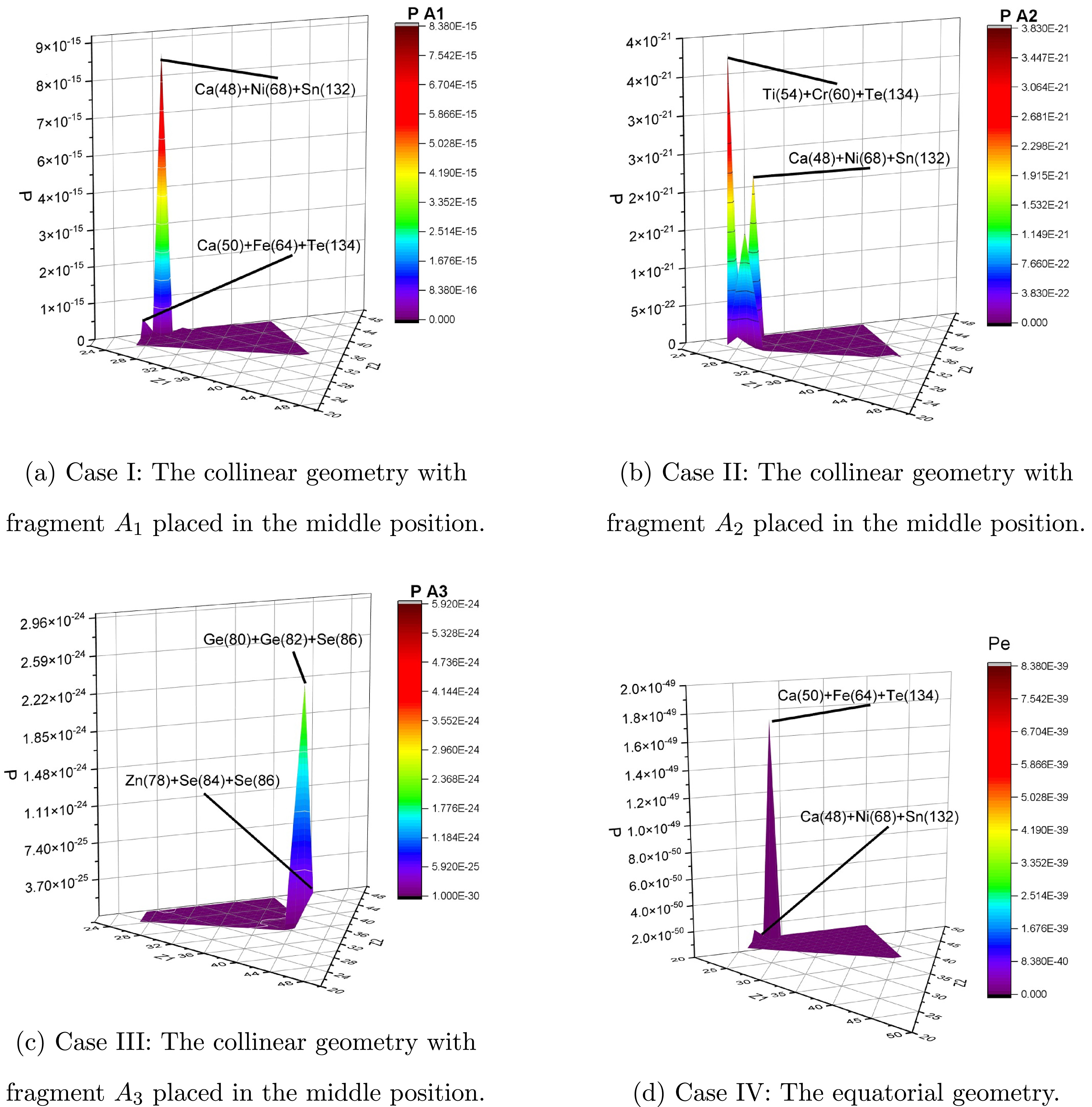
Figure 4. (color online) Penetrating probability via the atomic numbers of three fragments
$Z_1$ ,$Z_2$ , and$Z_3$ in various geometries for the ternary fission of the 248Cf isotope.In contrast, placing the lightest fragment,
$A_1$ , in the middle position (Case I, Fig. 4(a)) resulted in lower driving potentials, making these configurations more favorable. This is evidenced by their relatively short half-life of$8.100 \times 10^{5}$ s. When considering neutron emission, the half-life increased to$ 3.58 \times 10^{9} $ s. Similar trends have been reported in previous studies, such as those by Vijayaraghavan et al. [33, 56] and Karpov et al. [71], where the central placement of the lightest fragment was shown to minimize the driving potential and maximize penetration probability due to the decrease in Coulomb repulsion. These works serve as examples that corroborate our findings. Moreover, combinations such as$^{48}{\rm{Ca}}$ +$^{68}{\rm{Ni}}$ +$^{132}{\rm{Sn}}$ and$^{50}{\rm{Ca}}$ +$^{64}{\rm{Fe}}$ +$^{134}{\rm{Te}}$ presented in this paper further exhibited high stability due to the presence of double-magic fragments like$^{132}{\rm{Sn}}$ .Configurations with
$ A_2 $ located in the middle (Case II, Fig. 4(b)) exhibited intermediate behavior, with driving potentials and penetration probabilities influenced by the structural properties of the fragments. This is evidenced by its calculated half-life of$ 1.00339 \times 10^{12} $ s when considering neutron emission and$ 1.43 \times 10^{16} $ s when not considering neutron emission. Examples include the$ ^{54}\text{Ti} $ +$ ^{60}\text{Cr} $ +$ ^{134}\text{Te} $ and$ ^{48}\text{Ca} $ +$ ^{68}\text{Ni} $ +$ ^{132}\text{Sn} $ combinations, illustrating the stabilizing effects due to magic, near-magic, and even-even structures of fragments.By considering neutron emission, the reduction of Q-value led to an increase in the driving potential across all geometries. Consequently, the penetration probability decreased. Conversely, the geometry exhibited the same effect as when we did not consider neutron emission—the lighter the middle fragment, the higher the penetration probability. Additionally, the structural effects in the favored combinations, such as magic or near-magic shells, play a significant role in determining the most favorable sets of combinations. As shown in all collinear cases by considering neutron emission, the structural effects are critical in influencing the stability and penetrability of the configurations.
The equatorial geometry (Case IV, Fig. 4(d)) displays distinct behavior, with the longest calculated half-life of
$ 1.04 \times 10^{42} $ s, indicating exceptional stability. Combinations such as$ ^{50}\text{Ca} $ +$ ^{64}\text{Fe} $ +$ ^{134}\text{Te} $ and$ ^{48}\text{Ca} $ +$ ^{68}\text{Ni} $ +$ ^{132}\text{Sn} $ benefit from the presence of even-even, magic, and double-magic fragments, which further enhance their stability.Overall, our analysis revealed that the collinear fragments geometry is consistently more favorable than the equatorial fragmentation for true ternary fission, particularly when the middle fragment exhibits magic or near-magic properties. The placement of fragments and their nuclear structure critically influence barrier characteristics, penetration probabilities, and overall fission dynamics. These insights provide a deeper understanding of the mechanisms governing the ternary fission and emphasize the importance of structural configurations in predicting the half-life of ternary fission and its stability.
Study of the true ternary fission of 248Cf isotope in equatorial and collinear geometries
- Received Date: 2025-01-10
- Available Online: 2025-07-15
Abstract: This paper presents a comprehensive investigation of the true ternary fission of the


 DownLoad: