Traversable wormholes in AdS and entanglement

Similar to a black hole, a wormhole is a fascinating solution to Einstein's equations that has attracted significant interest in the theoretical physics community. Notably, it plays a crucial role in recent breakthroughs concerning the black hole information paradox [1, 2]. Generally, there are two types of wormholes: non-traversable and traversable. A well-known example of a nontraversable wormhole is the Einstein-Rosen bridge [3], which connects two asymptotic regions of eternal black holes. According to the ''ER=EPR'' conjecture [4], it is dual to entangled Einstein–Podolsky–Rosen (EPR) pairs, indicating a profound connection between wormholes and quantum entanglement. Traversable wormholes were first studied by Ellis [5] and Bronnikov [6] and then by Morris and Thorne [7]. However, these traversable wormholes generally violate the averaged null energy condition (ANEC), raising questions about their existence. It is important to note that the violation of ANEC can be accommodated through quantum fluctuations, such as the Casimir effect, which is considered acceptable. Nevertheless, the traversable wormhole described by Morris and Thorne permits time travel to the past, which contradicts the law of causality [8]. The first traversable wormhole consistent with causality was proposed by Gao, Jafferis, and Wall using a double trace deformation [9]. In this model, it takes longer to travel through the wormhole throat than it does via the typical path outside. Thus, this traversable wormhole adheres to the principles of causality and may be realized in the physical world. A significant advancement in this area is given by the humanly traversable wormholes proposed by Maldacena, Milekhin, and Popov, which use Casimir-like energy from fermions or the Randall-Sundrum brane-world scenario [10, 11]. Following this, wormhole solutions to Einstein's gravity coupled with Maxwell fields and two Dirac fermions were discovered [12] and refined in subsequent studies [13, 14]. Remarkably, this traversable wormhole is composed entirely of non-exotic matter. See also [15−18] for recent developments on wormholes.

This study extends the findings of [12, 13] from flat space to AdS space. We explored the CFT duals of traversable wormholes within the framework of the AdS/CFT correspondence [19]. We numerically solved the AdS wormholes with spherical and planar topologies according to Einstein-Dirac-Maxwell theories. We confirmed that these solutions violate the NEC. Therefore, they are genuine wormhole solutions. Additionally, we examined the holographic entanglement entropy (HEE) [20] of strips and disks on the two AdS boundaries of wormholes. As the size of the strip or disk grows, the Ryu-Takayanagi (RT) surface [20] for entanglement entropy undergoes a phase transition, transitioning from a disconnected state to a connected one. Interestingly, for the disk, the connected extremal surface only appears when the disk radius surpasses a critical value. We validate this unusual phenomenon using a toy model, confirming its occurrence in the case of the planar wormhole as well.

Let us outline the motivations for investigating the HEE in the wormhole background. First, HEE plays a crucial role in AdS/CFT. It reveals a deep connection between geometry and quantum entanglement [20]. From the first law of entanglement entropy, one can derive the linear Einstein equations in the framework of AdS/CFT [21, 22]. Furthermore, recent breakthroughs in the black hole information problem benefit from the development of HEE, particularly the concept of entanglement islands [1, 2]. Second, ''ER=EPR'' shows that the nontraversable wormhole is closely related to the entanglement entropy [4]. Thus, it is interesting to explore whether there are any connections between the traversable wormhole considered in this study and entanglement entropy. Third, the fermions on both sides of the flat wormhole are entangled [12]. Thus, the entanglement exploration of both sides of the AdS wormhole conducted in this study is of interest.

This paper is organized as follows. In Section II, we briefly review the Einstein-Dirac-Maxwell (EDM) model. In Section III, we numerically solve the EDM model to obtain traversable AdS wormholes with spherical and planar topologies, respectively. Section IV examines the HEE of strips in the AdS wormhole and discusses the phase transition. Section V generalizes the discussion to the HEE of disks. Finally, we conclude with a discussion in Section VI.

This section briefly reviews the Einstein-Dirac-Maxwell model, which contains one vector field, $ A_{\mu} $, and two spinor fields, $ \Psi_1 $ and $ \Psi_2 $. The action reads [12]

where we set Newton's constant as $ G_N=1 $, $ R $ is the Ricci scalar, $ l $ is the AdS radius, $ \mathcal{F}_{\mu\nu}=\partial_{\mu}A_{\nu}-\partial_{\nu}A_{\mu} $ is the field strength of the vector, and

Here, $ \gamma_{\mu}\equiv e_{\mu a}\hat{\gamma}^{a} $; $ \hat{\gamma}^{a} $ and $ \gamma_{\mu} $ are the gamma matrices in curved and flat spaces, respectively; $ e_{\mu a} $ are tetrad fields; $ m $ is the spinor mass, and

where $ \omega_{\mu ab} $ denotes the spin connections. The gamma matrices in flat space read [13]

where $ \sigma_i $ denotes the Pauli matrices:

From the action expressed in Eq. (1), we derive the equations of motion (EOMs):

where the stress-energy tensor is

with the Maxwell and Dirac-field stress-energy tensors defined as follows:

We solve the EOMs (Eqs. (6a)−(6c)) in the next section to obtain the traversable wormhole in AdS.

By solving the Einstein-Dirac-Maxwell model (Eq. (1)), we obtain the traversable wormhole solutions with spherical and planar topologies in an asymptotically AdS spacetime, as explained below.

For the wormhole with spherical topology, we assume the following ansatz of metric:

where ${\rm d}\Omega^2$ denotes the line element of unit sphere and $ r\ge r_0 $, with $ r_0 $ being the radius of wormhole throat. For numerical convenience, we parameterize $ r $ as [13]

Then, the metric becomes

As $ x $ goes from $ -1\to 0 \to 1 $, the radial coordinate $ r(x) $ goes from $ \infty \to r_0\to \infty $, which moves from one AdS boundary through the wormhole throat to the other AdS boundary. To have an asymptotically AdS spacetime, we impose the following boundary conditions:

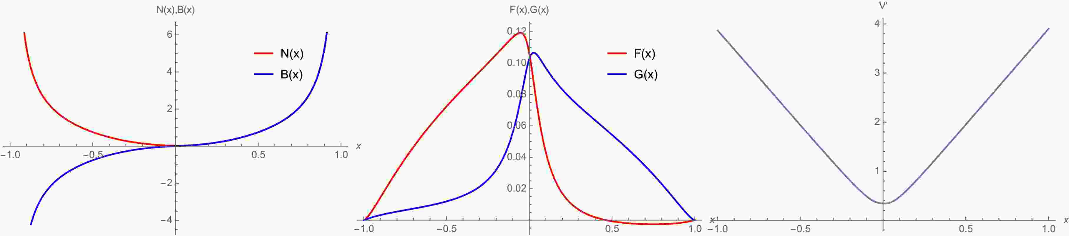
where a numerical cutoff of $ x=\pm (1-\epsilon) $ must be applied. We assume $ \epsilon=10^{-4} $ in this section. Note that we have $\mathop \lim_{x\rightarrow \pm1}N(x)^2=\lim_{x\rightarrow \pm1}B(x)^2\to \infty$ for AdS wormholes (see Fig. 1), while $ \lim_{x\rightarrow \pm1}N(x)^2=\lim_{x\rightarrow \pm1}B(x)\to 1 $ for flat wormholes [12−14]. This is the main difference between our wormhole solutions and those presented in [12−14] for flat space.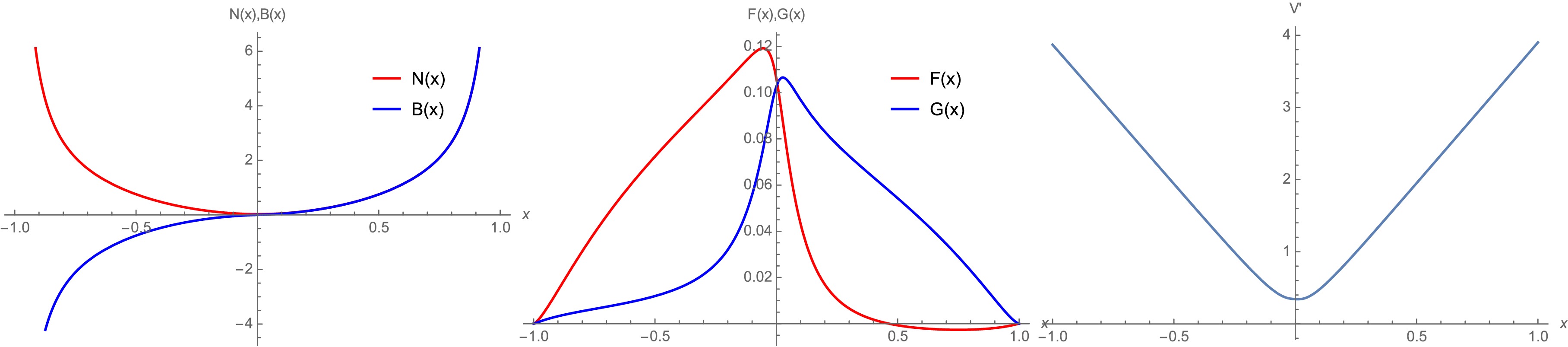

Figure 1.  (color online) Wormhole with spherical topology. The theory parameters and initial values are given by Eqs. (18) and (19).

From the metric expressed by Eq. (10), we read off the tetrad fields:

We employ the following ansatz for the vector,

whereas for the spinors,

where

with $ F(x),G(x) $ being real functions. Substituting the above ansatzs into the EOMs (Eqs. (6a)−(6c)), we obtain a set of ordinary differential equations for $N(x),\;B(x), V(x),\;F(x)$, and $ G(x) $ (see Appendix A). These are first-order equations for $ F(x) $, $ G(x) $, $ N(x) $, and $ B(x) $ and second-order equations for $ V(x) $.

We apply the shooting method to solve the wormhole solutions. To do so, we expand $ A=(F,G,N,V,B) $ around the throat $ x=0 $,

which means that $ B(x)=b_0+b_1 x+O(x^2) $, with similar expressions for other functions $ (F,G,N,V) $. Solving EOMs perturbatively, we obtain the following constraints:

For any given set of initial values in Eq. (14), we can numerically solve the EOMs (see Appendix A) to obtain a solution. In general, this solution does not obey the asymptotical boundary conditions (Eqs. (11a) and (11b)) at $ |x|\to 1 $. We adjusted the initial values in Eq. (14) to satisfy the boundary conditions (Eqs. (11a) and (11b)). This is the so-called shooting method. Without loss of generality, we set the theory parameters as

and found the following initial values:

The corresponding functions for the wormhole are represented in Fig. 1. As shown in Fig. 2, the wormhole solution obeys the boundary conditions (Eqs. (11a) and (11b)) on the asymptotically AdS boundary $ |x|\to 1 $. For instance, numerically, we have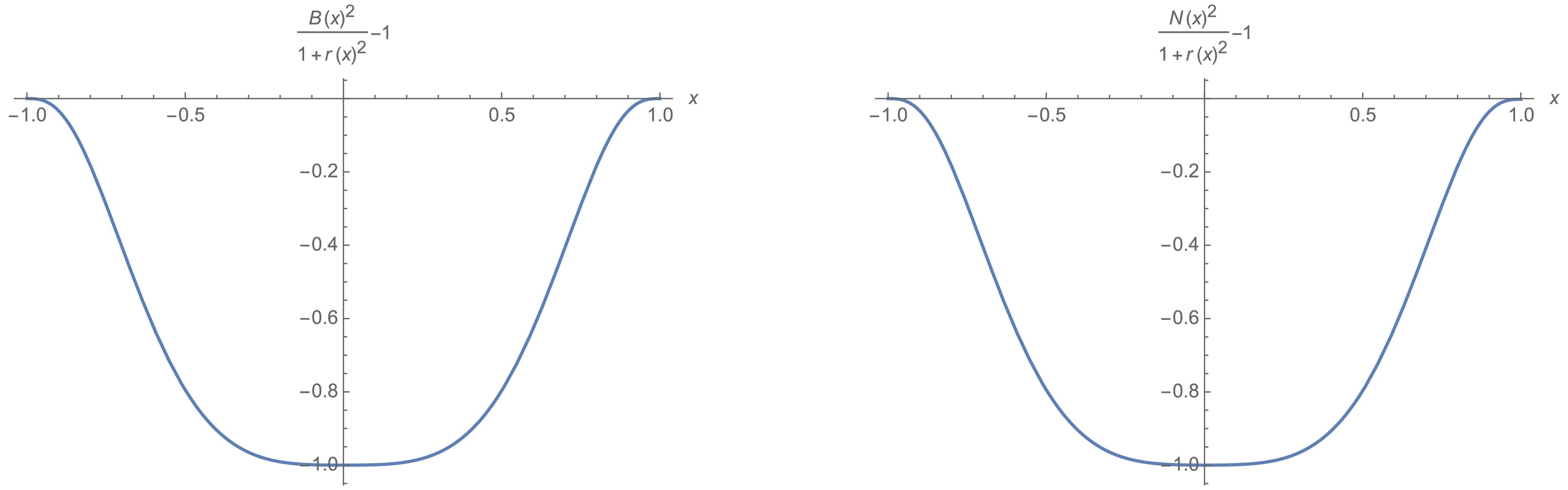

Figure 2.  (color online) Asymptotically-AdS conditions expressed by Eqs. (11a) and (11b) satisfied.

on the AdS boundary $ |x|=1-10^{-4} $. Note that the last term in Eq. (21) does not vanish perfectly. According to [12], it implies that there is a slight redshift on the right AdS boundary.

To examine the fermion distributions, we can calculate the charge density given by

which is represented in Fig. 3. This plot indicates that the charge is distributed throughout the entire space, reaching a maximum near the throat ($ x=0 $) and gradually approaching zero at the AdS boundary ($ |x|=1 $).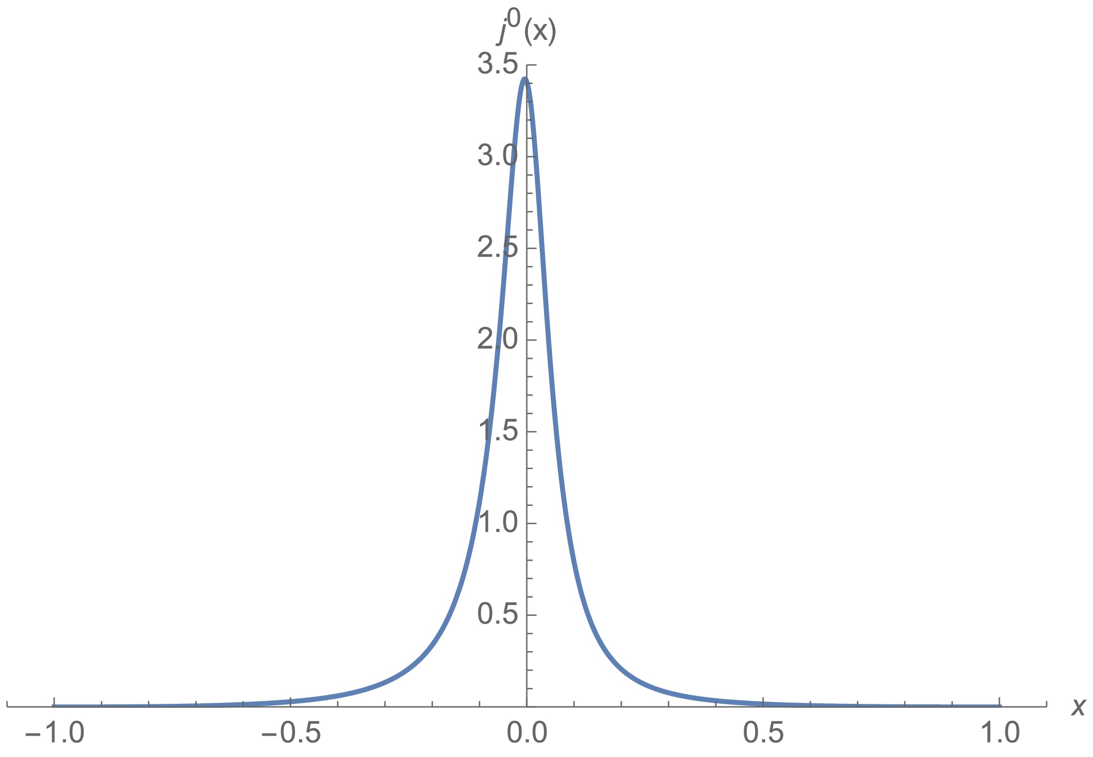

Figure 3.  (color online) Charge density of spherical wormhole. The charge is distributed throughout the space (consistent with Pauli exclusion principle), reaching a maximum near the throat ($ x=0 $) and gradually approaching zero at the AdS boundary ($ |x|=1 $).

It is well-known that a traversable wormhole violates the null energy condition (NEC). For the null vector

we verified that the NEC is violated for our wormhole solution, i.e., $ T_{\mu\nu}K^{\mu}K^{\nu}<0 $ (see Fig. 4). Thus, we obtained a traversable wormhole in the asymptotically AdS spacetime. Figure 4 shows that the NEC is most severely violated near the throat of the wormhole, $ x\to 0 $, while it is essentially not violated near the AdS boundary, $ x\to \pm 1 $. More precisely, we numerically observed that the NEC is violated in the bulk region, $ -0.67<x<1 $.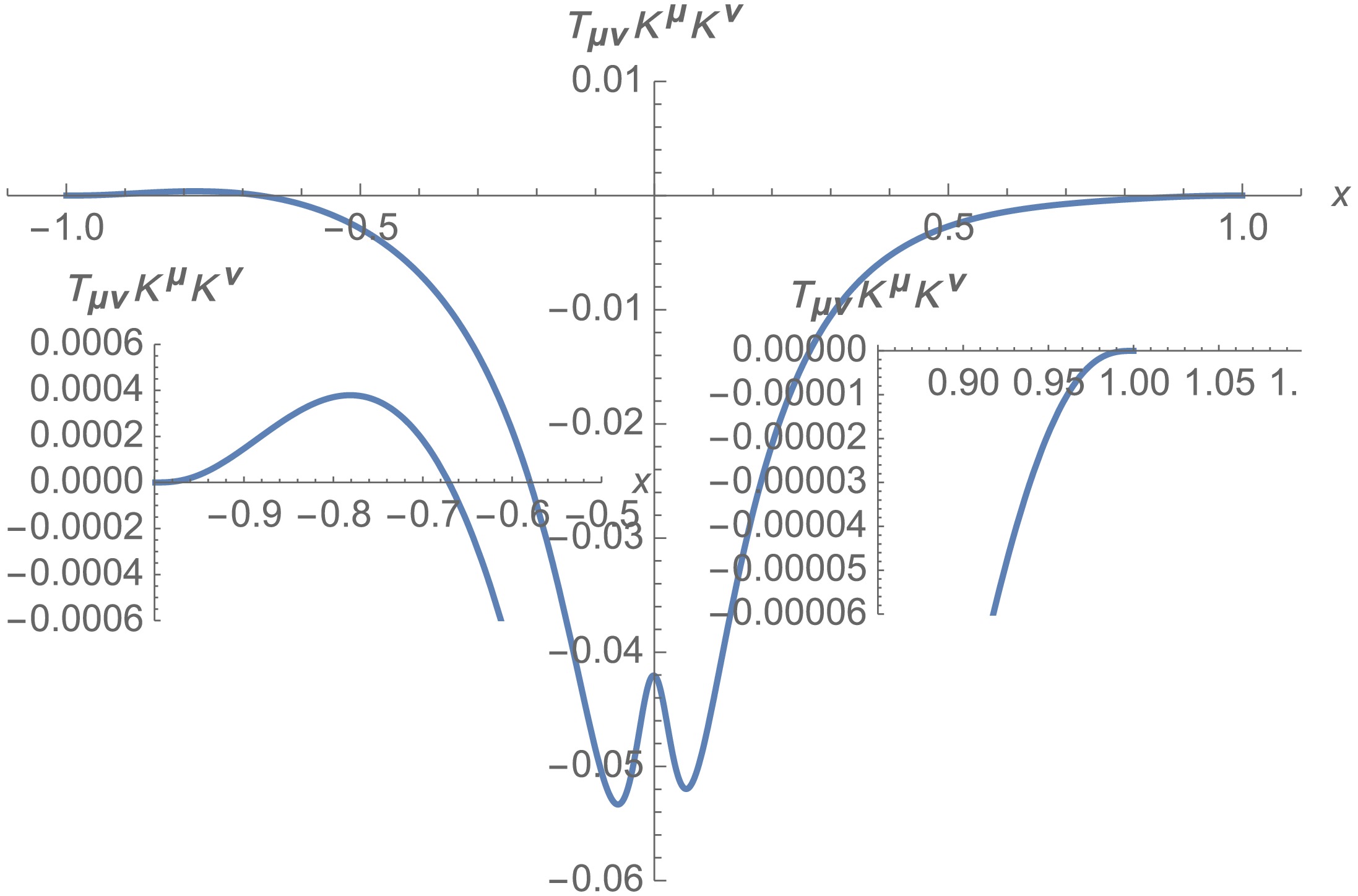

Figure 4.  (color online) Violation of the NEC for the wormhole with spherical topology, i.e., $ T_{\mu\nu}K^{\mu}K^{\nu}<0 $.

Let us proceed to study the wormhole with planar topology. Given that the calculations are similar to those for spherical topology, we only highlight key points below. We adopted the following ansatz for the metric:

where we set the AdS radius $ l=1 $ for simplicity. Eq. (24) must be an asymptotically-AdS metric:

From Eq. (24), we obtain the tetrads:

The ansatz for vector and spinors are given by Eq. (13a) and

Substituting Eqs. (13a), (13d), (27a), and (27b) into the EOMs given by Eqs. (6a)−(6c), we obtain a set of ordinary differential equations for $ N(x),B(x),V(x),F(x) $, and $ G(x) $ (see Appendix B). Solving these EOMs perturbatively around the throat $ x=0 $, we obtain

We set the parameters and initial values using the shooting method as follows:

A typical solution of the planar wormhole and charge density is shown in Fig. 5. We verified the violation of the NEC shown in Fig. 6, i.e., $ T_{\mu\nu}K^{\mu}K^{\nu}<0 $. We numerically found that the NEC is violated in the bulk region, $ -0.76<x<1 $. We conclude that the shorter the distance to the wormhole throat, the more severe the NEC violation.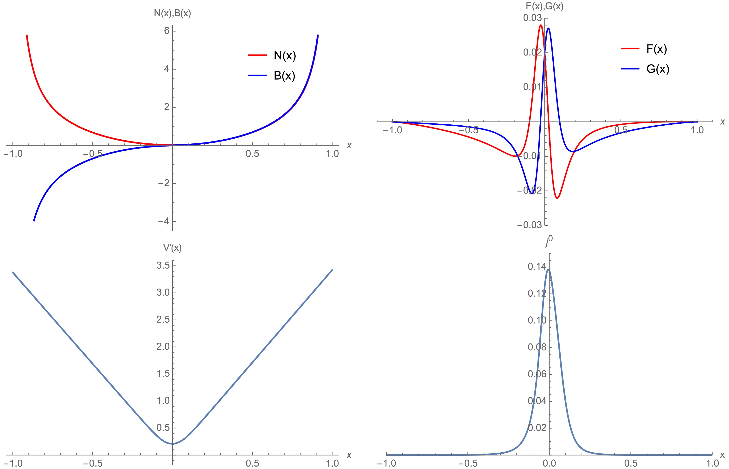

Figure 5.  (color online) Planar wormhole and charge density with parameters set according to Eq. (31).

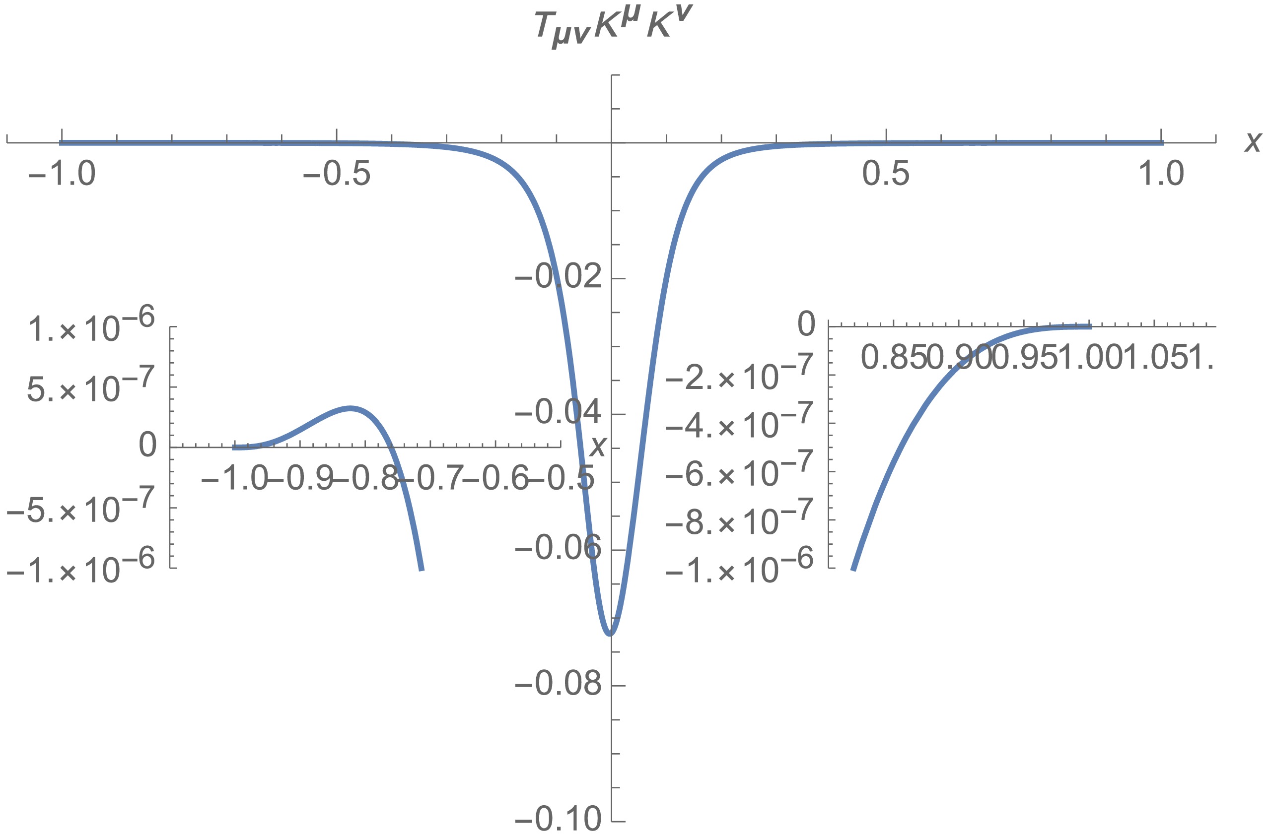
Figure 6.  (color online) Violation of the NEC for the wormhole with planar topology, i.e., $ T_{\mu\nu}K^{\mu}K^{\nu}<0 $.

As shown in Fig. 7, the wormhole solution properly obeys the boundary conditions on the asymptotically AdS boundary $ |x|\to 1 $. For instance, we numerically have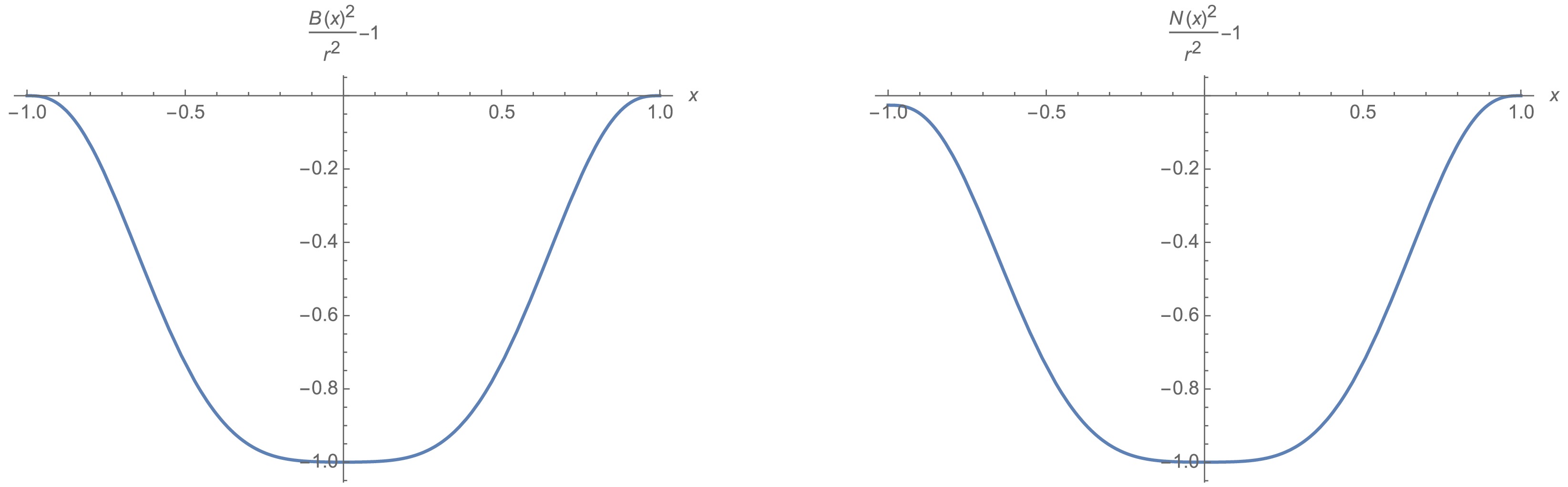

Figure 7.  (color online) Asymptotically-AdS conditions (Eqs. (25a) and (25b)) are satisfied up to a redshift.

where we have redefined time as $ t\rightarrow 0.99 t $ to make $ (N^2/r^2)|_+\to 1 $ on the right AdS boundary. Then, we have $ (N^2/r^2)|_-\approx 0.97 $ on the left AdS boundary, which can be explained as a redshift [12].

In this section, we investigate the HEE [20] of two strips on the two AdS boundaries of the traversable wormhole. For simplicity, we focus on the planar topology. As shown in Fig. 8, there are two phases for the RT surfaces: connected and disconnected.

Figure 8.  (color online) Phase transition of RT surface. As the strip width (red line segment) increases, the RT surface (blue curve) transforms from a disconnected phase (left) to a connected phase (right).

Recall that the HEE can be calculated using the area of the minimal surface (RT surface) in bulk [20] as follows:

where $ A $ denotes the subsystem on the AdS boundary, and $ \gamma_A $ is the minimal surface in bulk whose boundary coincides with that of $ A $, i.e., $ \partial \gamma_A=\partial A $. For the strip $ -L/2\le y_1\le L/2 $, the embedding function of RT surface in bulk is assumed to be

Then, we derive the induced metric of the RT surface

with area

where we set $\int {\rm d}y_2=1$. Given that$ \mathcal{L} $ includes no $ y(x) $, we can define a conserved quantity:

Let us first discuss the disconnected phase (red curve inFig. 9), which dominates for small strip widths. As shown in Figs. 8 and 9, there is a turning point $ x_{\text{min}} $ for the disconnected phase. At this point, we have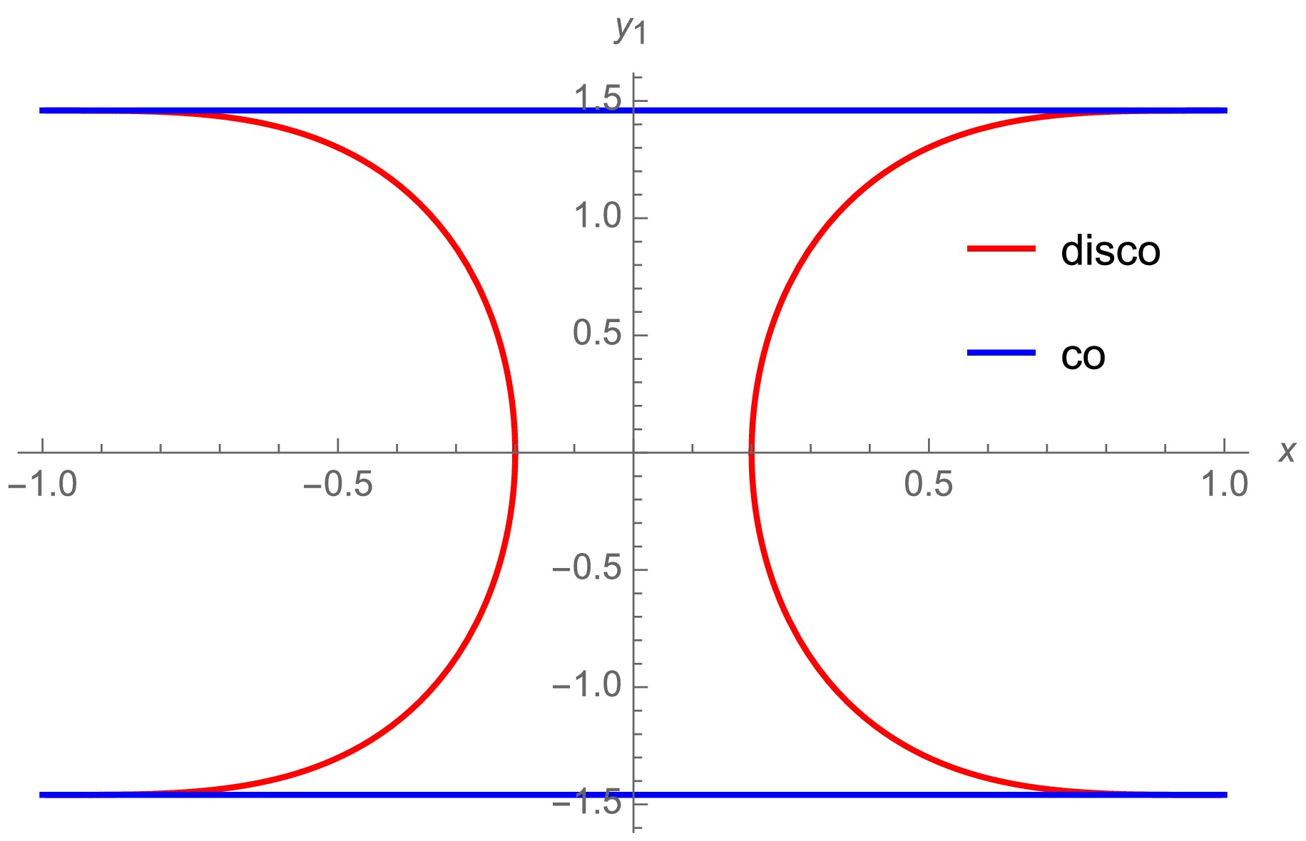

Figure 9.  (color online) Two types of extremal surfaces with strip width $ L=1.48 $. The red and blue curves correspond to the disconnected and connected phases, respectively.

Substituting Eq. (39) into Eq. (38), we obtain

On the right hand side of the wormhole ($ x>0 $), we can use Eqs. (38) and (40) to solve $ y'_1(x) $ and obtain the strip width:

We set the same strip width $ L $on the left hand side of the wormhole ($ x<0 $). Note that $ |x_{\min}| $ is slightly different on the two sides of the wormhole given that $ |B(x)| $ is not exactly symmetric.

Substituting $ y'(x) $ into Eq. (37), we obtain the area of extremal surface, $ \mathcal{A}_{\text{disco}}=\mathcal{A}_{\text{disco},x>0}+\mathcal{A}_{\text{disco},x<0} $, with

where $ |x_{\min}| $is not exactly the same on the two sides of the wormhole.

Let us proceed to discuss the connected phase (blue curve of Fig. 9), which dominates for large strip widths. According to Eq. (38), we observe that the solution for the connected phase is $ y_1'(x)=0 $. Then, the area of the extremal surface becomes

which is constant for fixed wormhole geometry.

By definition, the RT surface is given by the extremal surface with minimal area. As $ x_{\min} $ decreases, both the strip width $ L $ described by Eq. (41) and the area of extremal surface $ \mathcal{A}_{\text{disco}} $ described by Eqs. (42) and (43) increase. Thus, for sufficiently large $ L $, $ \mathcal{A}_{\text{disco}} $ could be larger than $ \mathcal{A}_{\text{co}} $. Then, there is a phase transition and the connected phase dominates. The $ \delta \mathcal{A}-L $ relation is represented in Fig. 10, where $ \delta \mathcal{A}=\mathcal{A}_{\text{disco}}-\mathcal{A}_{\text{co}} $. This figure shows that the disconnected phase dominates for $ \delta \mathcal{A}<0 $ and small values of $ L $, while the connected phase dominates for $ \delta \mathcal{A}>0 $ and large values of $ L $. A phase transition of the RT surface occurs near the strip width, that is, $ L\approx 1.61 $.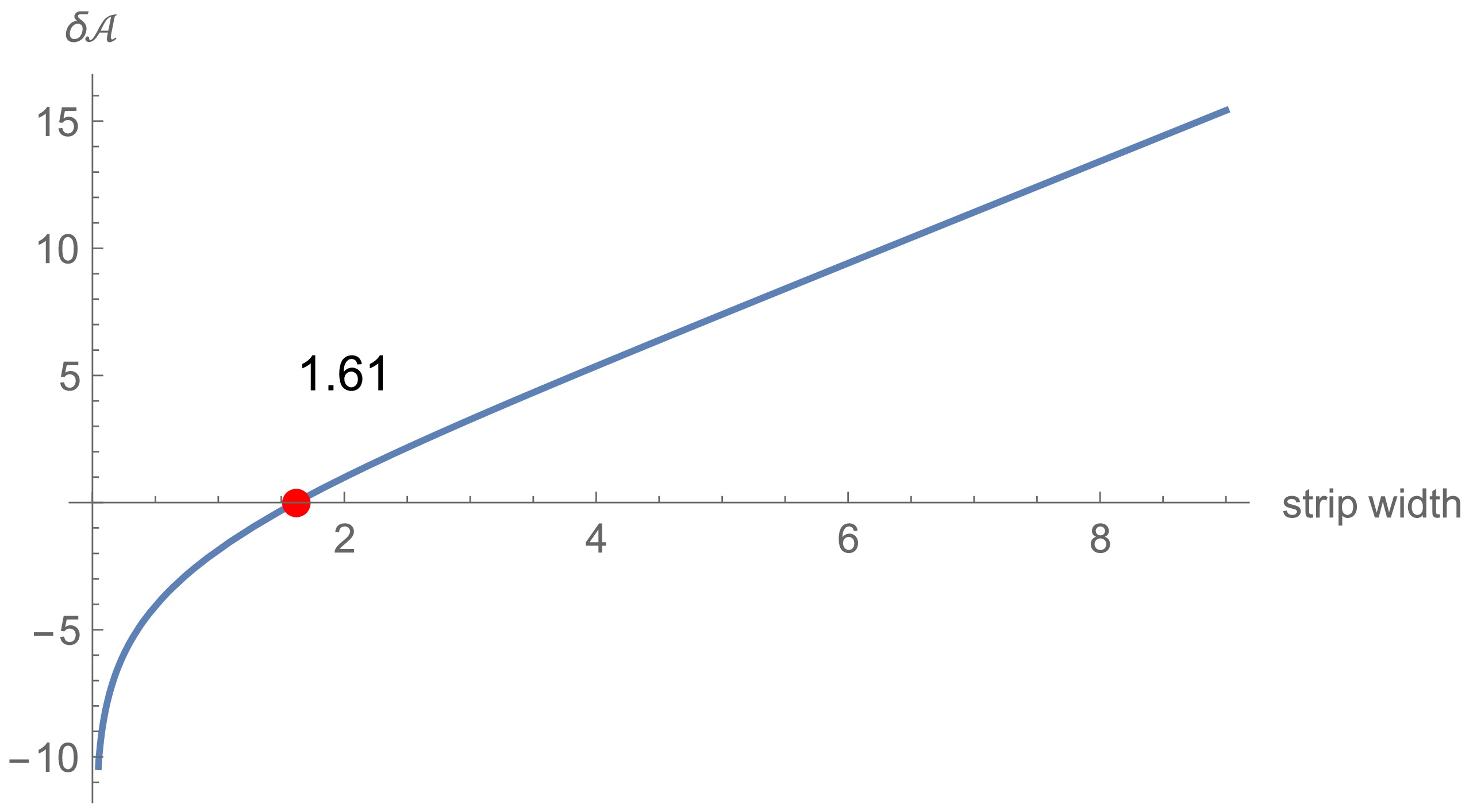

Figure 10.  (color online) Area difference ($ \delta \mathcal{A}=\mathcal{A}_{\text{disco}}-\mathcal{A}_{\text{co}} $) increasing with strip width $ L $. The disconnected and connected phases dominate for $ L<1.61 $ and $ L>1.61 $, respectively.

To conclude this section, let us comment on the possible relationship between the NEC and phase transition of holographic entanglement entropy. Recall that the NEC is most severely violated near the wormhole's throat. Similarly, the HEE undergoes a phase transition when the RT surface extends deeply into the bulk region near the wormhole throat. Thus, it is natural to ask whether the violation of the NEC causes the phase transition of holographic entanglement entropy. This is qualitatively correct. For instance, the turning point of the disconnected extremal surface at the phase-transition point is $ \left|x_{\text{min}}\right|\approx 0.37 $, localized in the region violating the NEC. However, we found no exact relation between the NEC and phase transition of HEE. It lies beyond the scope of this study. This is an open question to be addressed in future studies.

This section examines the HEE of disks on the two AdS boundaries of the planar wormhole. A key feature is that the connected extremal surface disappears when the disk radius is sufficiently small. This is similar to the case of an eternal black hole [23], where the Hartman-Maldacena (HM) surface of a disk vanishes after a sufficiently long time. In contrast, for a strip, there is always a connected extremal surface for a wormhole and an HM surface for an eternal black hole. We first illustrate this unusual phenomenon using an analytical toy model and then extend the results to our numerical wormhole.

Let us start with a toy model with the metric

which violates the NEC

and approaches $ \text{Poincar}\acute{\text{e}} $-AdS for $ \tilde{r}\rightarrow \infty $. This is a wormhole in an asymptotically AdS space. Note that it is not a solution to the Einstein-Dirac-Maxwell model (Eq. (1)). We consider the unusual situation of HEE for a disk with $ \rho\le L $. As in Section 2, we define

and assume the embedding function of the RT surface in bulk:

Then, the induced metric on the RT surface reads

From Eq. (49), we derive the area functional of the RT surface as

where the integral is performed on one side of the wormhole and a factor of $ 2 $ is added to account for the whole space. This area functional yields the following Euler-Lagrange equation:

Similar to the strip case, there are disconnected and connected extremal surfaces for the disk, where the corresponding boundary conditions read

Here,$ x_{\text{min}} $is the turning point of disconnected extremal surfaces; Fig. 11 shows an example. Without loss of generality, we set $ a=r_0=1 $. The connected phase occurs only if the disk radius is larger than a critical value, i.e., $ L\ge 1.28 $. The critical value is represented by a green point in Fig. 12, which shows one disk radius generally corresponding to two or three different extremal surfaces. We set the one with minimal area as the RT surface.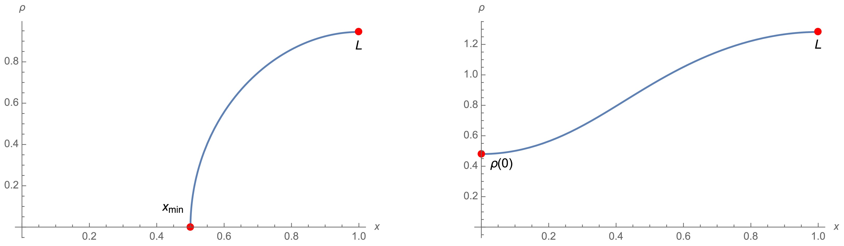

Figure 11.  (color online) Disconnected (left) and connected (right) extremal surfaces of disks for $ x > 0 $. Here, $ x_{\text{min}} $ is the turning point of the disconnected extremal surface and $ L=\rho(1) $ is the disk radius.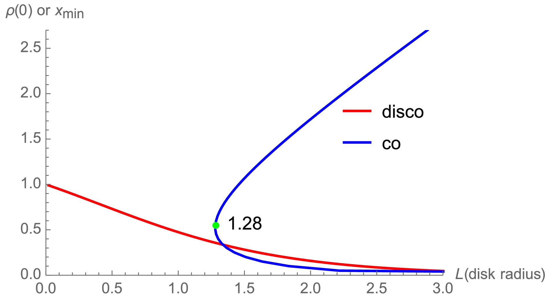

Figure 12.  (color online) Disk radius of minimal value (green point) for the connected phase. Generally, one disk radius corresponds to one disconnected surface and two connected surfaces.

The area difference $ \delta \mathcal{A}=\mathcal{A}_{\text{disco}}-\mathcal{A}_{\text{co}} $ is represented in Fig. 13; note that $ \delta \mathcal{A} $ increases with the disk radius $ L $. The disconnected and connected phases dominate for $ L<1.40 $ and $ L>1.40 $, respectively. Note that the critical point, $ L_c\approx 1.28 $, for the existence of the connected phase is smaller than the phase-transition point, $ L_p\approx 1.40 $. It aligns with the expectation that, for a sufficiently large disk size, the connected phase invariably dominates. In such a scenario, the extremal surface would traverse through the wormhole throat.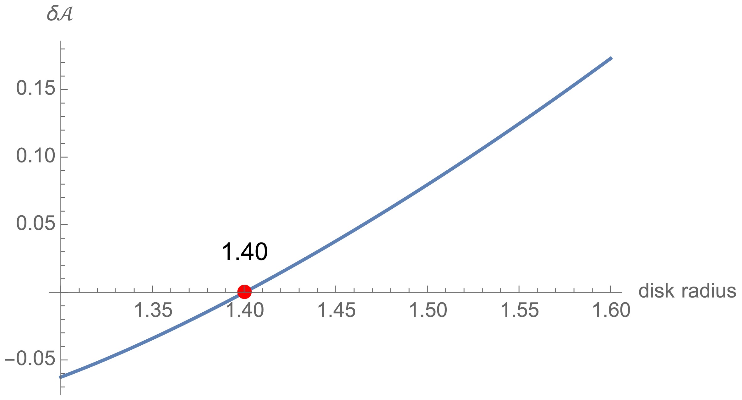

Figure 13.  (color online) Existence of phase transition (red point); the area difference $ \delta \mathcal{A}=\mathcal{A}_{\text{disco}}-\mathcal{A}_{\text{co}} $ increases with the disk radius $ L $. The disconnected and connected phases dominate for $ L<1.40 $ and $ L>1.40 $, respectively.

Next, we study the HEE of disks for the planar wormhole obtained in Sec. III.B. Because the discussions are similar to those of toy model, we list only key results below. Similar to the toy model, the connected extremal surface exists only if the disk radius is larger than one critical value, $ L\ge L_c $. As shown in Fig. 14, we have $ L_c\approx 4.68 $. Besides, as shown in Fig. 15, one disk radius corresponds to several extremal surfaces when $ L>L_c $. Unlike the toy model with $ L_c<L_p $, the area of the connected extremal surface, if it exists, is always smaller than that of disconnected extremal surface. In Fig. 14, we subtract a universal UV divergence for all areas, i.e., $\dfrac{L}{ \epsilon}$($ \epsilon=10^{-4} $). Thus, the critical radius $ L_c $ is also the phase-transition point $ L_p $ of disconnected and connected phases.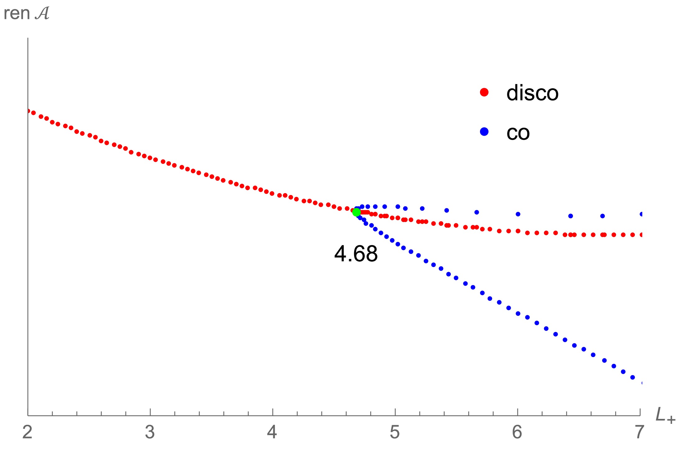

Figure 14.  (color online) Relation between the renormalized area $ ( \mathcal{A}-\frac{L}{\epsilon}) $ and right disk radius $ L_+ $. For $ L_+< L_c\approx 4.68 $, only the disconnected phase exists, and we set $ L_-=L_+ $. For $ L_+>L_c\approx 4.68 $, $ L_- $ can be determined by $ L_+ $ in the connected phase, which is slightly different from $ L_+ $ owing to the slight asymmetry of the two sides of the wormhole. Fig. 16 shows the differences between $ L_+ $ and $ L_- $.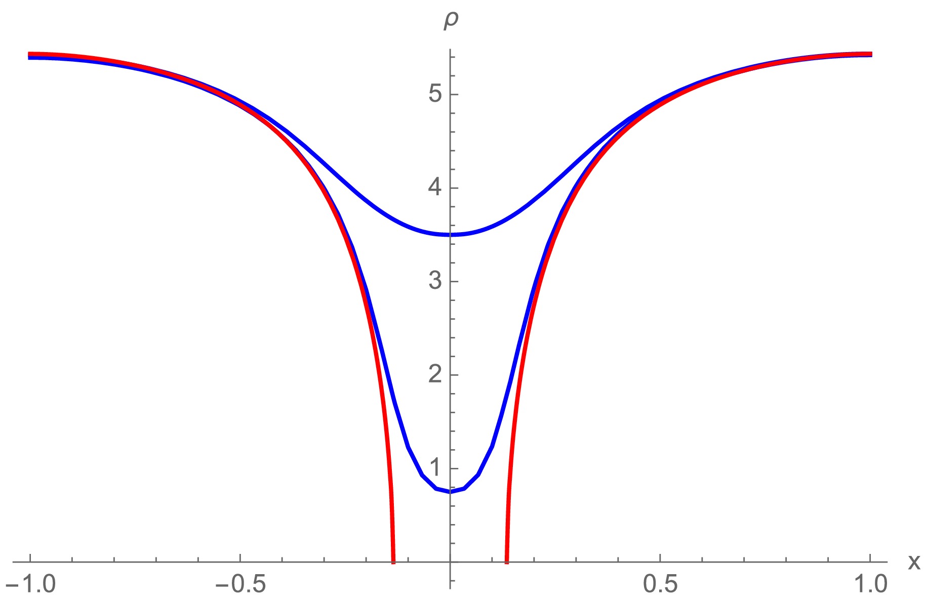

Figure 15.  (color online) Extremal surfaces with disk radius $ L_+\simeq L_-\approx 5.43 > L_c $. Note that the disk radius corresponds to several extremal surfaces for $ L>L_c $. We set the one with minimal area as the RT surface.

Note that, according to the asymmetric wormhole solution, the BC given by Eq. (54) results in slightly different disk radii on either side of the wormhole in the connected phase; see Fig. 16 for example, where the differences between $ L_+ $ and $ L_- $ are small. As shown in Fig. 14, when $ L_+ < L_c \approx 4.68 $, only the disconnected phase exists, enabling the condition $ L_+ = L_- $ to be set freely. However, for $ L_+ > L_c \approx 4.68 $, the connected phase dominates, and $ L_- $ is determined by $ L_+ $, which generally differs from $ L_+ $. Fortunately, this difference is negligible, as demonstrated in Fig. 16. Similar to the toy model discussed in Section V.A, the connected extremal surface appears only when the disk radius exceeds a critical value, $ L > L_c $. Unlike the toy model, the critical disk radius represents the phase-transition point between the disconnected and connected phases, that is, $ L_c = L_p $.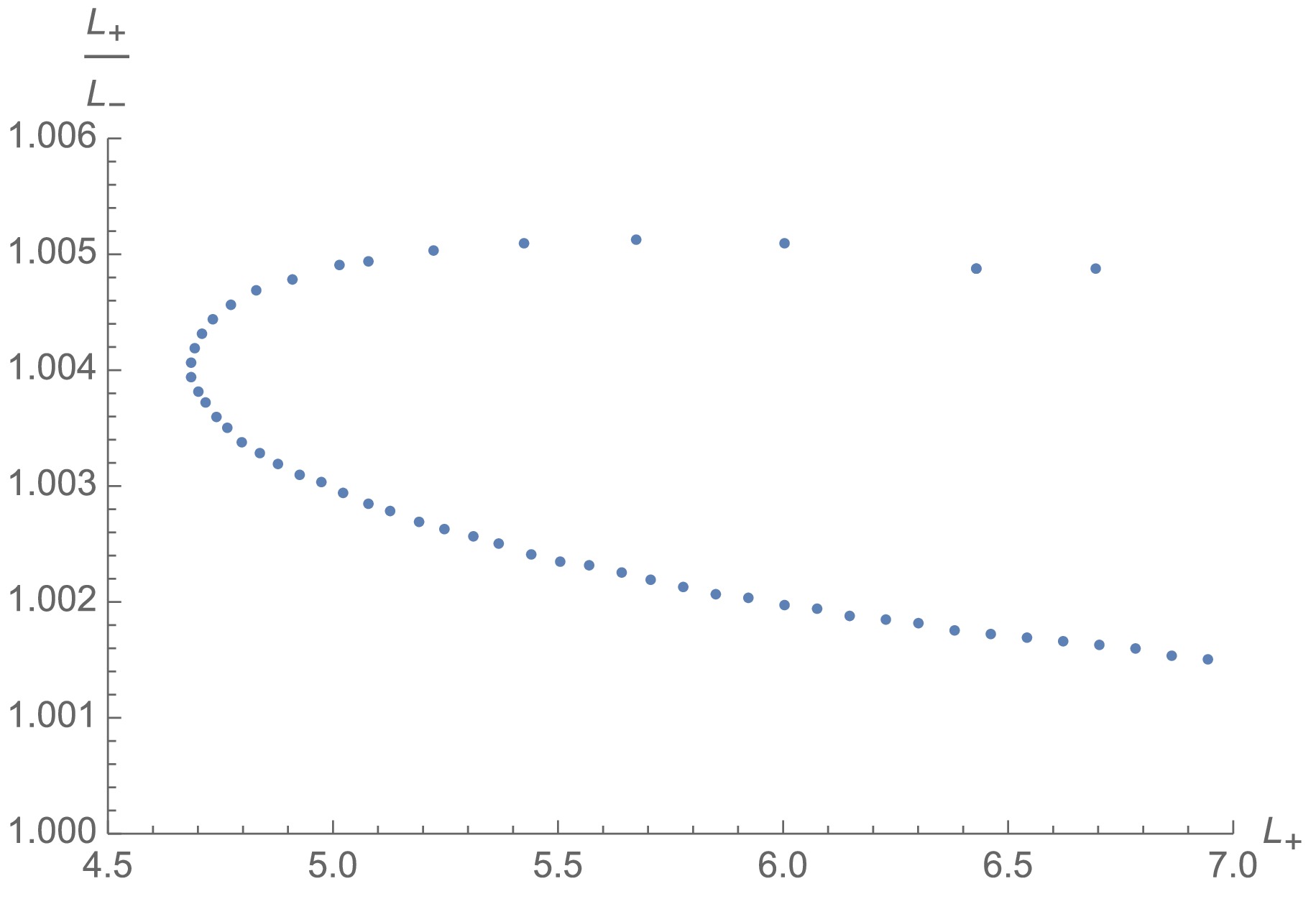

Figure 16.  (color online) Differences in disk radii for the connected phase. It shows that the differences between $ L_- $ and $ L_+ $are extremely small.

Traversable wormholes have recently been obtained in the Einstein-Dirac-Maxwell model without exotic matter. In this study, we extended the discussion to AdS spacetime and derived traversable wormholes with spherical and planar topologies. Additionally, we investigated the holographic entanglement entropy of strips and disks for traversable AdS wormholes. As the size of the strip or disk increases, the Ryu-Takayanagi (RT) surface for entanglement entropy undergoes a phase transition, shifting from a disconnected phase to a connected phase. Interestingly, for the disk, the connected extremal surface exists only when the disk radius exceeds a critical value. We validated this novel phenomenon using a toy model, confirming its occurrence in the case of the planar wormhole as well. Furthermore, we express interest in exploring the hyperbolic wormhole and examining the quantum entanglement of dual conformal field theories (CFTs) in future research.

We thank Y. Q. Wang and S. W. Wei for their valuable comments and discussions.

This appendix lists the EOMs of the Einstein-Dirac-Maxwell model for the AdS wormhole with a spherical topology.

This appendix lists the EOMs of the Einstein-Dirac-Maxwell model for the planar AdS wormhole. Here, we set $ l=1 $.