Model-independent constraints on the Hubble constant using lensed quasars and the latest supernova

Incorporating the cosmological principle and accommodating the notion of inflation to elucidate the early universe's rapid expansion, the standard cosmological model, also known as the ΛCDM model, has stood as the prevailing framework to comprehend the large-scale structure, composition, and evolution of the universe. Over the past several decades, the ΛCDM model has demonstrated extraordinary success in reproducing observational phenomena across diverse cosmic epochs. Its predictions have shown remarkable agreement with key cosmological probes, including the cosmic microwave background (CMB) radiation, baryon acoustic oscillations (BAOs), and Type Ia supernovae (SNe Ia), among others. Despite its successes, the standard cosmological model has faced significant challenges. Notable among these are the large scale alignment of quasar polarization vectors [1], reported spatial variations in the fine-structure constant [2, 3], alignments observed in the low multipoles of the CMB angular power spectrum [4−6], and the persistent Hubble tension [7, 8].

Thereinto, the Hubble constant $ H_0 $, a fundamental parameter representing the current rate of expansion of the Universe, provides insights into the universe's size, age, and evolution. Thus, it is important to accurately measure the Hubble constant. Within the framework of the ΛCDM model, Planck Collaboration utilized measurements of the CMB radiation, employing the temperature and polarization anisotropies to infer the Universe parameters [9], in which the Hubble constant is constrained as $ H_0 = 67.4\pm0.5 $ km s⁻¹ Mpc⁻¹. The result is embraced by the obtained value from measurements of the combination of BAO [10−12]. While Riess et al. [13] determined the Hubble constant of $ H_0 = 74.03\pm1.42 $ km s⁻¹ Mpc⁻¹ with the Cepheid distance ladder, which is inconsistent with the value inferred from Planck CMB by more than 4.4σ. This discrepancy between the Hubble constant values inferred from the local distance ladders and from early universe observations, namely ''the $ H_0 $ tension problem'', seems to herald the existence of new physics beyond the standard cosmological model if the possibility of systematic errors in observations is ruled out. This discrepancy has encouraged researchers to determine $ H_0 $ with other independent cosmological probes [14−18].

Strong gravitational lensing (SGL) system with time delay is one of the most promising cosmological probes to resolve the tension because of its inverse relationship with $ H_0 $. Strong gravitational lensing is a phenomenon predicted by Einstein's general theory of relativity, where the gravitational field of a massive object, such as a galaxy or a galaxy cluster, bends the path of light from a background source, typically the active galactic nuclei (AGN). When the alignment between the foreground object and the AGN is nearly perfect, the light from the AGN is bent and magnified, creating distorted and often multiple images of the AGN. Since the light from each image of the AGN follows a different path as it travels through the gravitational potential of the lens, time delay is introduced to describe the time difference between the lights of two images arriving on Earth. The time delay can be accurately measured from the light curves of any two images by monitoring the variability in the brightness of the AGN over time.

From the analysis of time delay, precise determination of the lensing potential derived from high-resolution imaging techniques, and considering the effects of the line-of-sight environment, the ''time-delay distance'' $ D_{\Delta t} $ can be determined. This distance is a ratio relating to three angular diameter distances and has a scale of $ H_0 $; hence, it can always be employed to infer $ H_0 $. The lensing program H0LiCOW ($ H_0 $ Lenses in COSMOGRAIL’s Wellspring) aims to precisely determine$ H_0 $by combining data from gravitational lens systems with state-of-the-art modeling techniques [19]. It should be noticed that the dimensionless distance between the observer, lens, and source should be determined before inferring $ H_0 $ with the time-delay distance. In a spatially flat ΛCDM model, the H0LiCOW collaboration found$ H_0 = 72.0^{+2.3}_{-2.6} $ km s⁻¹ Mpc⁻¹ at a precition of 3% with four lens systems [20]. Recently, the H0LiCOW collaboration updated their constraint to $ H_0 = 73.3^{+1.7}_{-1.8} $ km s⁻¹ Mpc⁻¹ at 2.4% precision [21] using a lens dataset consisting of six multiply-imaged quasar systems [20, 22−27]. Furthermore, the TDCOSMO (Time-Delay COSMOgraphy) collaboration has investigated the systematic uncertainties in the inference of $ H_0 $ using a sample of six lens systems from H0LiCOW supplemented by the SGL system DES J040-5354, which has a precisely measured time-delay distance [28−30]. By leveraging this expanded sample, TDCOSMO determined $ H_0 $ with an improved precision of 2.2% within a flat ΛCDM framework, finding no evidence of bias or errors surpassing the current statistical uncertainties [31, 32]. However, these results are model-dependent and vary with the cosmological models [21]. To model-independently determine $ H_0 $, Collett et al. [33] employed a fourth-order polynomial to fit the Pantheon SNe Ia data to obtain the dimensionless distance and obtained the constraint $ H_0 = 74.2^{+3.0}_{-2.9} $ km s⁻¹ Mpc⁻¹ at a precision of 4% within four strong lensing systems. On the other hand, Liao et al. [34, 35] employed another model-independent method, the Gaussian process (GP) method, to reconstruct an unanchored luminosity distance from the Pantheon data. In a flat universe, they obtained $ H_0 = 72.2\pm2.1 $ km s⁻¹ Mpc⁻¹ with four lens systems and $ H_0 = 72.8^{+1.6}_{-1.7} $ km s⁻¹ Mpc⁻¹ with six lens systems. As we can see, besides the quantity of lens samples, the methods used to determine the distance, that is, assuming a certain cosmological model, a polynomial function and the GP method, affect the constraint of $ H_0 $.

Deep learning has emerged as a transformative tool in cosmology, leveraging its ability to process extensive datasets and uncover intricate patterns within them. Among its techniques, artificial neural networks (ANNs) function as latent models trained on observational data to characterize underlying properties with high precision. Recent advancements have demonstrated the efficacy of deep learning in a range of cosmological applications, including data reconstruction [36−39], yielding notable progress. In this work, we will apply deep learning to explore the Hubble tension. Given that different reconstruction techniques yield varying constraints on cosmological parameters [38, 39], we will employ several well-established data reconstruction techniques, including deep learning, Gaussian Process regression, polynomial fitting, and Padé approximant, to reconstruct the unanchored luminosity distance using the latest Pantheon+ compilation of 1701 SNe Ia light curves [40]. By combining these reconstructions with SGL data from the TDCOSMO sample, we aim to assess the impact of reconstruction approaches on $ H_0 $ constraints.

This paper is structured as follows: In Section II, we describe the datasets utilized in this study, including SGL systems and SNe Ia, along with the methods employed to reconstruct the unanchored luminosity distance from SNe Ia. Section III details the methodology for determining the Hubble constant $ H_0 $, and presents the corresponding results. Finally, discussions and conclusions are given in Section IV.

Strong gravitational lensing (SGL) is one of the most important phenomenon in the Universe and a powerful tool for measuring the distribution of matter at different scales, obtaining information about the large scale structure of the Universe, determining fundamental cosmological parameters and so on. In partucular, time-delay is sensitive to the Hubble constant $ H_0 $, as first proposed by Refsdal [41]. For a single lens plane, the arrival time of light from an image at θ on Earth is delayed compared to the time it would take if the light traveled in a straight path without deflectors. The time delay between two images is the difference in their individual time delays, expressed as

where c is the speed of light and $ \Delta \phi $ is the Fermat potential difference between the two images with respect to the parameter of lens mass profile $ {\boldsymbol{\xi}}_{\mathrm{lens}} $. $ D_{\Delta t} $ is the time-delay distance, which is related to three angular diameter distances

where $ z_d $ is the redshift of lens. $ D_d $, $ D_s $ and $ D_{ds} $ are the angular diameter distances between the lens and observer, the source and observer, the lens and source, respectively. In a spatially flat universe, $ D_{ds} $ can be simply written as [35, 42, 43]

where $ z_s $ is the redshift of a source. Assuming a certain cosmological model, the angular diameter distance can be obtained and further used to determine$ H_0 $, combining the time-delay distance observation released by the H0LiCOW project [21]. Additionally, the angular diameter distance $ D_d $can also be determined by the light profile $ {\boldsymbol{\xi}}_{\mathrm{light}} $, the projected stellar velocity dispersion $ \sigma^P $, and the anisotropy distribution of the stellar orbits parameterized by $ \beta_{\mathrm{ani}} $ [20],

where J is the function capturing all the model components computed from angles measured in the sky and the stellar orbital anisotropy distribution.

The H0LiCOW collaboration is dedicated to accurately measuring the Hubble constant $ H_0 $ using the SGL of multiply-imaged quasars. The project utilizes a combination of observational data, including high-resolution imaging and spectroscopy, along with sophisticated modeling techniques to extract the precise measurements of $ H_0 $. Recently, their latest work has employed their latest sample of six H0LiCOW systems to investigate $ H_0 $ in different cosmological models and obtained $ H_0 = 73.3^{+1.7}_{-1.8} $ km s⁻¹ Mpc⁻¹ at a precision of 2.4% in the standard flat ΛCDM model. The TDCOSMO collaboration reanalyzed a new sample of seven SGL systems, six of which are derived from the H0LiCOW dataset, referred to as the TDCOSMO sample. This analysis has led to a high-precision determination of$ H_0 $ with an uncertainty of 2.2% within the framework of a flat ΛCDM cosmology [31, 32]. This TDCOSMO has five lenses (RXJ1131−1231, PG 1115+080, B1608+656, SDSS 1206+4332 and DES J0408-5354) with both$ D_{\Delta t} $ and $ D_d $ measurements, and two lenses (HE 0435−1223 and WFI2033−4723) with $ D_{\Delta t} $ measurements only. The posterior distributions of distances are made available in two formats: Markov Chain Monte Carlo (MCMC) chains or fits based on skewed log-normal functions. These resources can be accessed on the H0LiCOW website ¹ and Refs. [28, 29]. We present their redshifts and relevant distances in Table 1.

Lens	$ z_l $	$ z_s $	$ D_{\Delta_t} $ (Mpc)	$ D_d $ (Mpc)	Reference
RXJ1131$ - $1231	0.295	0.654	$ 2096_{-83}^{+98} $	$ 804_{-112}^{+141} $	[23, 26]
PG 1115+080	0.311	1.722	$ 1470_{-127}^{+137} $	$ 697_{-144}^{+186} $	[26]
HE 0435-1223	0.4546	1.693	$ 2707_{-183}^{+168} $	$ ... $	[24, 26]
DES J0408$ - $5354	0.597	2.375	$ 3382_{-115}^{+146} $	$ 1711_{-280}^{+376} $	[28, 29]
B1608+656	0.630	1.394	$ 5156_{-236}^{+296} $	$ 1228_{-151}^{+177} $	[22, 25]
WFI2033-4723	0.6575	1.662	$ 4784_{-399}^{+248} $	$ ... $	[27]
SDSS 1206+4332	0.745	1.789	$ 5769_{-471}^{+589} $	$ 1805_{-398}^{+555} $	[20]

Table 1.  Redshifts and distances of the seven SGL systems ordered by lens redshifts.

To determine $ H_0 $ using Eq. (2), three angular diameter distances for each SGL system must be derived. Following the approach of Liao et al. [34, 35], we reconstruct the expansion history $ H(z)/H_0 $ from SNe Ia without assuming a specific functional form. This reconstruction allows us to calculate the unanchored luminosity distances in a spatially flat universe as

The corresponding angular diameter distances are then obtained using the relation

In this work, we reconstruct the distances from the latest Pantheon+ compilation [44], which comprises 1701 light curves from 1550 unique SNe Ia spanning a redshift range of $ 0.001<z<2.3 $. Multiple model-independent methods are employed to explore the impact of these approaches on the determination of $ H_0 $.

Deep learning (DL) has proven to be a robust approach for addressing complex problems and processing large datasets, with demonstrated success in reconstructing data through the training of artificial neural networks (ANNs) [36−39]. In this study, we design a deep neural network (DNN) architecture comprising an input layer that accepts redshift vectors as features, an output layer that predicts the unanchored luminosity distance, and three hidden layers that mediate the transformation of information. The hidden layers consist of 200 neurons in the first and third layers and 400 neurons in the second layer. A nonlinear activation function, the Rectified Linear Unit (ReLU), is employed to enhance the performance of the neural network. The ReLU function is defined as follows:

The architecture of our DNN is depicted in Fig. 1, and the mathematical formulation for each layer is outlined below:

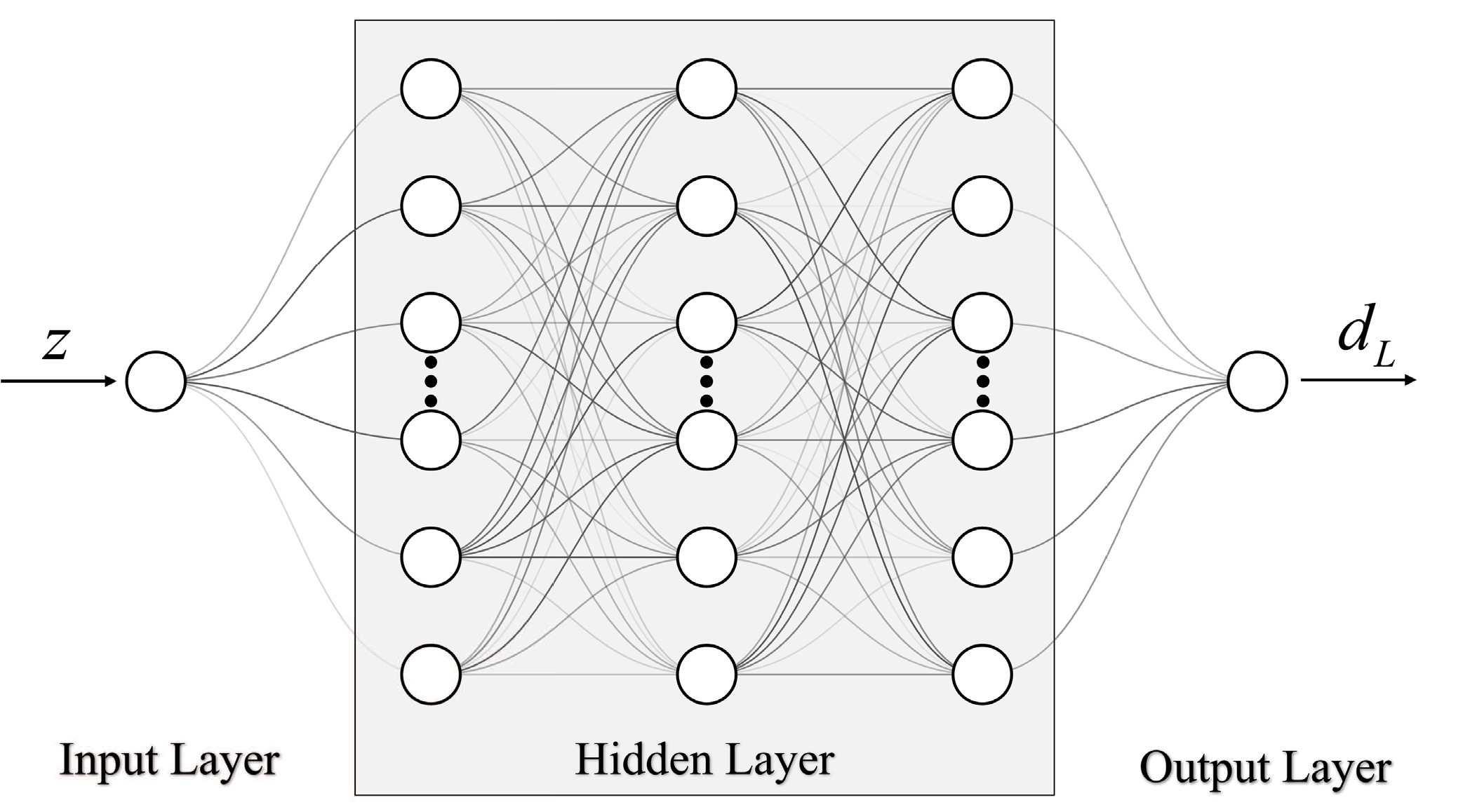
Figure 1.  The architecture of the DNN featuring three hidden layers. The input consists of the redshift values, while the output corresponds to the associated unanchored luminosity distances. The number of neurons in each layer is represented by the number of circles.

1) Input layer:

where z is the redshift vector.

2) Hidden layers :

where $ {\boldsymbol{W}}_i $ and $ {\boldsymbol{b}}_i $ represent the weight matrix and bias vector of the i-th hidden layer, with dimensions $ m\times n $ and $ m\times 1 $, respectively. Here, m and n correspond to the number of neurons in the i-th layer and its preceding layer.

3) Output layer:

where W is a $ 1\times 200 $ weight matrix, and b is a bias vector corresponding to the output layer.

The DNN is optimized by minimizing a loss function, specifically the mean squared error (MSE), which quantifies the discrepancy between predicted and observed distances. The Adam optimizer is employed to efficiently identify the loss function's minimum. To estimate prediction uncertainties, we incorporate the dropout technique, a regularization method. Dropout layers with a rate of 0.1 are placed after the first and third hidden layers. Previous studies [36, 37] have demonstrated that networks employing dropout can approximate Bayesian models, offering a simpler alternative to traditional Bayesian networks while retaining comparable predictive capabilities [45]. It is worth noting that, while previous works have proposed various network architectures for reconstructing data from diverse observations, such as the RNN+BNN network [36, 37] and ReFANN network [46], our DNN differs from these approaches. Compared to the RNN+BNN network, our DNN is better suited to handle the particular characteristics of the Pantheon+ dataset, where the redshifts of some SNe Ia in the low redshift range are closely spaced. Moreover, our DNN requires significantly fewer neurons than the ReFANN network, enabling the faster training of the optimal model.

Liao et al. [35] employed Gaussian process (GP) regression to reconstruct the unanchored luminosity distance from the Pantheon dataset, obtaining a constraint on the Hubble constant of $ H_0 = 72.8^{+1.6}_{-1.7} $ km s⁻¹ Mpc⁻¹ for a flat universe. In this work, we adopt GP regression as the second method to reconstruct the unanchored luminosity distance. GP regression is a non-parametric technique for reconstructing a function $ y = f(x) $ from the observations $ (x_i,y_i) $. A GP is formally defined as a stochastic process in which the function values follow a multivariate Gaussian distribution:

where $ {\boldsymbol{x}} = \{x_i\} $, $ {\boldsymbol{y}} = \{y_i\} $, μ is the mean of the Gaussian distribution, C is the covariance matrix of the data, and $ {{\bf{K}}}({\boldsymbol{x}},{\boldsymbol{x}}) $ is the kernel matrix encoding assumptions about the reconstructed function, with elements $[{{\bf{K}}}({\boldsymbol{x}},{\boldsymbol{x}})]_{ij} = k(x_i,x_j)$. Following Liao et al. [34], we use a squared-exponential covariance function:

where the hyperparameters $ \sigma_f $ (signal variance) and l (length scale) are optimized by maximizing the marginalized likelihood. Additionally, to explore the impact of the kernel function on the inference of $ H_0 $, we also implement the commonly used Matern covariance function:

where ν is a parameter controlling the smoothness of the resulting function, fixed at 1.5 in this work, Γ is the Gamma function, $ d_E $ is the Euclidean distance, and $ B_{\nu} $ is a modified Bessel function.

Collett et al. [33] adopted a fourth-order polynomial to fit the Pantheon dataset, constraining $ H_0 $at a precision of 4% in a flat universe by simultaneously fitting the coefficients of the polynomial and combining four strong lensing systems (B1608+656, RXJ1131-1231, HE 0435-1223, and SDSS 1206+4332). In this work, the polynomial fitting (polyfit) is the third reconstruction method. To ensure consistency with the GP and DNN methods, we first reconstruct the data using polyfit and then utilize the reconstructed data to constrain $ H_0 $. Although polynomial fitting is effective in local regions, it may encounter issues such as the Runge phenomenon, particularly at the data boundaries. The Padé approximant (PA), which utilizes rational functions (ratios of polynomials), provides a more robust solution for handling complex behaviors. Moreover, the PA method typically offer superior extrapolation capabilities, especially when the data demonstrates asymptotic or other non-polynomial trends. Therefore, we also employ the PA method to reconstruct the unanchored luminosity distance. A Padé approximant is a type of rational function used to approximate a given function and is represented as the ratio of two polynomials, typically in the form:

where m and n denote the degrees of the polynomials in the numerator and denominator, respectively.

We employ the above aforementioned methods to reconstruct the unanchored luminosity distance from the Pantheon+ dataset. Specifically, the DNN is trained using TensorFlow ², and GP regression is implemented using the publicly available Python package scikit-learn [47]. A fourth-order polynomial is utilized in the polyfit method, and the Padé approximant is of order (2, 1). The resulting reconstructions are shown in Fig. 2. The reconstructed unanchored luminosity distances exhibit variations in both the predicted values and their associated uncertainties, reflecting the inherent characteristics and limitations of each reconstruction method.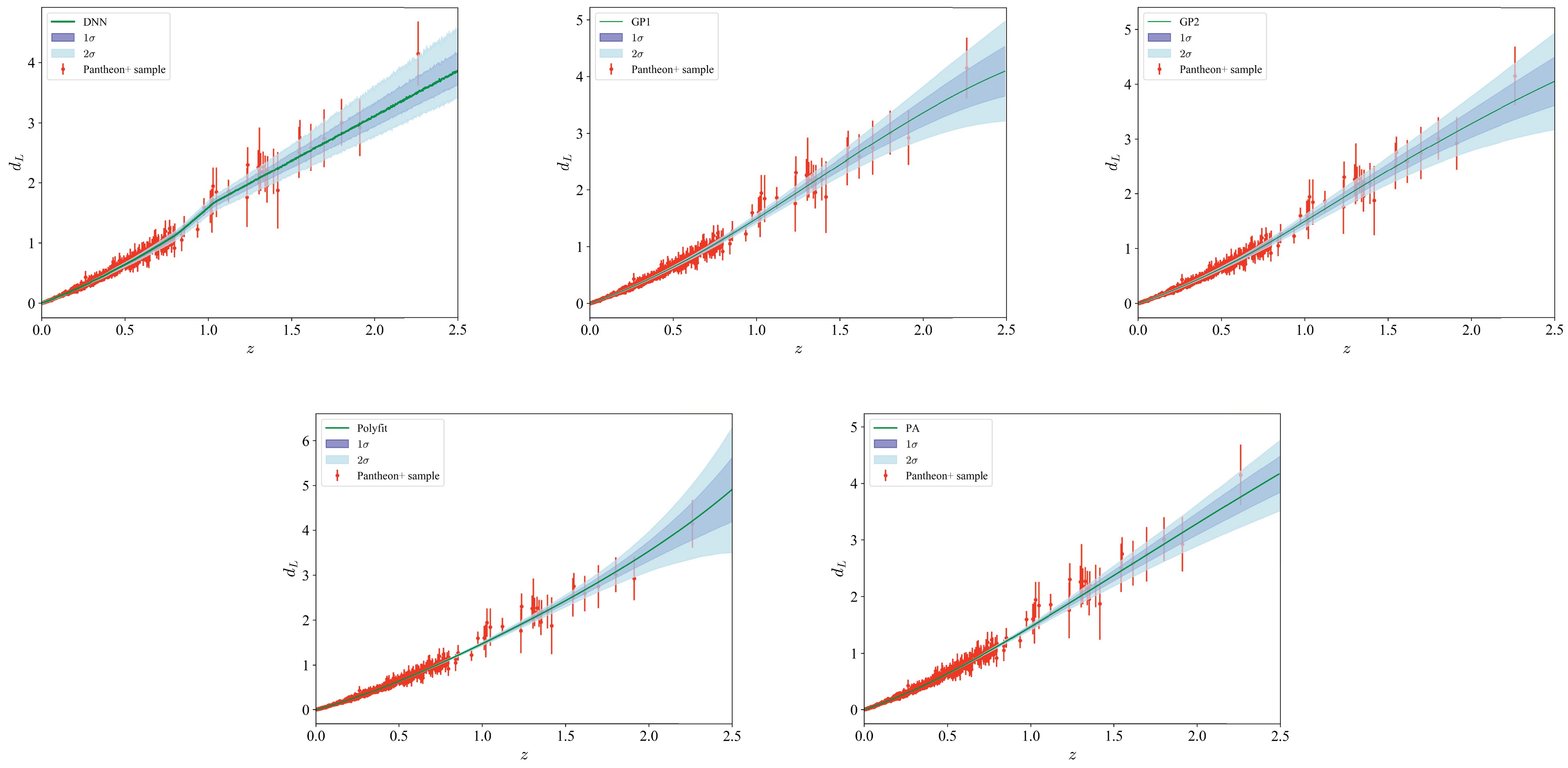

Figure 2.  (color online) Reconstructed unanchored luminosity distances $ d_L $ using the model-independent methods: deep neural networks (DNN), Gaussian process (GP)-GP1 with squared-exponential function and GP2 with Matern function, polynomial fitting (polyfit), and Padé approximant (PA).

The DNN method produces a smooth reconstruction that closely aligns with the Pantheon+ data points across the redshift range. Its uncertainties are relatively narrow at lower redshifts, where the data density is high but increase gradually at higher redshifts owing to sparser data coverage. Notably, the DNN reconstruction exhibits an elevated trend near a redshift of 1, likely driven by observations in that range. This behavior demonstrates the DNN's capacity to learn patterns directly from the observational data.

The GP methods also provides a strong fit to the data, particularly at low and intermediate redshifts. However, their uncertainties are slightly broader than those of the DNN method in the high redshift range, where data sparsity becomes more pronounced. These broader uncertainty bands reflect the non-parametric nature of GP regression, which allows for flexible interpolation but is sensitive to noise and sparsity in the dataset. The reliance of GP on the covariance structure becomes evident in regions with sparse data, where the lack of constraints leads to increased uncertainty. Additionally, a comparison of the reconstructions from the GP method with the squared-exponential kernel (GP1) and the Matern kernel (GP2) reveals that the inferred data remains largely unchanged despite the variation in the kernel function.

In contrast, the polyfit method yields a smoother reconstruction but shows notable deviations from the above two methods at higher redshifts. Its narrower uncertainty in low redshift and broader uncertainty in high redshift bands indicate limitations in capturing the detailed features of the dataset. The reliance on a predefined functional form restricts the adaptability of this method, making it susceptible to underfitting or overfitting, particularly in regions where the data distribution is sparse or complex. In comparison, the PA method demonstrates superior adaptability to the overall data characteristics, producing results that are more consistent with those obtained from DNN and GP methods. Notably, the PA approach offers superior extrapolation capabilities, addressing the limitations of the polyfit method, particularly at higher redshifts.

For a given SGL system, the time-delay distance, expressed in terms of $ H_0 $, can be written as:

where $ H_0D_d/c $ and $ H_0D_s/c $ are derived using Eq. (6) from the reconstructed unanchored luminosity distance at the lens redshift $ z_l $ and source redshift $ z_s $, respectively. The term $ H_0D_{ds}/c $ is subsequently computed using Eq. (3). By combining the observed time-delay distances $ D_{\Delta t} $ and, where available, angular diameter distances $ D_d $ from the H0LiCOW project, the Hubble constant $ H_0 $ can be determined. The procedure is as follows:

1) Calculate the joint likelihood of seven SGL systems with respect to $ H_0 $ using Eq. (17) (and Eq. (6)), by multiplying the likelihoods derived from the $ D_{\Delta t} $ observations (and $ D_d $, if available for specific systems) based on a given reconstructed curve.

2) Perform a Markov Chain Monte Carlo (MCMC) analysis to maximize the joint likelihood and compute the posterior probability density function (PDF) of the parameter space using the Python package $ \textsf{emcee}$ ³ [48].

3) Repeat the above steps for 1000 different reconstructed curves, generating 1000 chains of $ H_0 $.

4) Combine the chains to obtain the final posterior distribution of $ H_0 $.

The constraints on the Hubble constant $ H_0 $ derived from the seven SGL systems, as well as individual system results, are summarized in Table 2, with the corresponding posterior PDFs shown in Fig. 3. For all SGL systems, using the DNN reconstruction, the best-fit value for $ H_0 $ is $ H_0 = 72.3^{+3.8}_{-3.6} $ km s⁻¹ Mpc⁻¹, which is in good agreement with the local distance ladder measurement ($ H_0 = 74.03\pm1.42 $ km s⁻¹ Mpc⁻¹) but exhibits mild tension with the CMB constraints from Planck ($ H_0 = 67.4\pm0.5 $ km s⁻¹ Mpc⁻¹) owing to the slightly high uncertainty. When using the GP1 and GP2 reconstructions, $ H_0 $ is constrained to $ H_0 = 72.4^{+1.6}_{-1.7} $ km s⁻¹ Mpc⁻¹ and $ H_0 = 73.1^{+1.5}_{-1.6} $ km s⁻¹ Mpc⁻¹, achieving precisions of 2.3% and 2.2%, respectively. These values are also slightly higher than the CMB measurement, consistent with the DNN results, and provide relatively tighter constraints on $ H_0 $. The polyfit reconstruction yields $ H_0 = 70.7^{+3.0}_{-3.1} $ km s⁻¹ Mpc⁻¹, which is lower than the values obtained from the DNN and GP methods. In contrast, the PA reconstruction produces $ H_0 = 74.0^{+2.7}_{-2.7} $ km s⁻¹ Mpc⁻¹, which is marginally higher than the estimates from the other methods. For clarity, the best-fit $ H_0 $ values with corresponding 1σ uncertainties are illustrated in Fig. 4 with different colors denoting results obtained from different reconstructed datasets. For comparison, the $ H_0 $ constraints from the Planck Collaboration [9] and Riess et al. [13] are shown along with their 1σ and 2σ confidence intervals. In summary, the results obtained from these reconstruction methods are consistent within 1σ level and collectively indicate a preference for a higher $ H_0 $ value compared to the CMB constraints.

Methods	RXJ1131	PG1115	HE0435	DES J0408	B1608	WFI2033	SDSS 1206	All
DNN	$ 77.8^{+6.1}_{-5.7} $	$ 83.7^{+8.9}_{-7.9} $	$ 74.1^{+7.0}_{-6.5} $	$ 78.3^{+7.2}_{-7.2} $	$ 69.6^{+7.1}_{-6.5} $	$ 73.6^{+9.0}_{-8.2} $	$ 71.5^{+10.2}_{-8.5} $	$ 72.3^{+3.8}_{-3.6} $
GP1	$ 77.4^{+3.6}_{-3.6} $	$ 80.2^{+7.9}_{-7.0} $	$ 70.5^{+4.7}_{-4.5} $	$ 75.5^{+4.5}_{-4.3} $	$ 69.1^{+2.8}_{-3.1} $	$ 70.5^{+3.9}_{-4.9} $	$ 67.8^{+5.4}_{-4.9} $	$ 72.4^{+1.6}_{-1.7} $
GP2	$ 78.1^{+3.7}_{-3.8} $	$ 81.2^{+8.0}_{-7.1} $	$ 71.4^{+4.8}_{-4.5} $	$ 76.3^{+4.2}_{-4.1} $	$ 69.3^{+2.8}_{-3.1} $	$ 71.5^{+3.8}_{-4.9} $	$ 68.9^{+5.5}_{-4.9} $	$ 73.1^{+1.5}_{-1.6} $
Polyfit	$ 77.0^{+3.4}_{-3.4} $	$ 79.5^{+7.9}_{-7.0} $	$ 69.9^{+5.0}_{-4.7} $	$ 68.9^{+6.3}_{-4.9} $	$ 69.4^{+3.3}_{-3.4} $	$ 69.3^{+4.6}_{-5.2} $	$ 65.8^{+5.9}_{-5.3} $	$ 70.7^{+3.0}_{-3.1} $
PA	$77.1^{+3.4}_{-3.4} $	$80.9^{+8.1}_{-7.2} $	$71.9^{+5.3}_{-4.9} $	$75.2^{+5.0}_{-4.7} $	$71.1^{+3.8}_{-3.7} $	$72.5^{+5.1}_{-5.5} $	$69.1^{+6.0}_{-5.4} $	$74.0^{+2.7}_{-2.7} $

Table 2.  Best-fit parameters for $ H_0 $derived from all SGL systems combined and from individual systems using different reconstruction methods.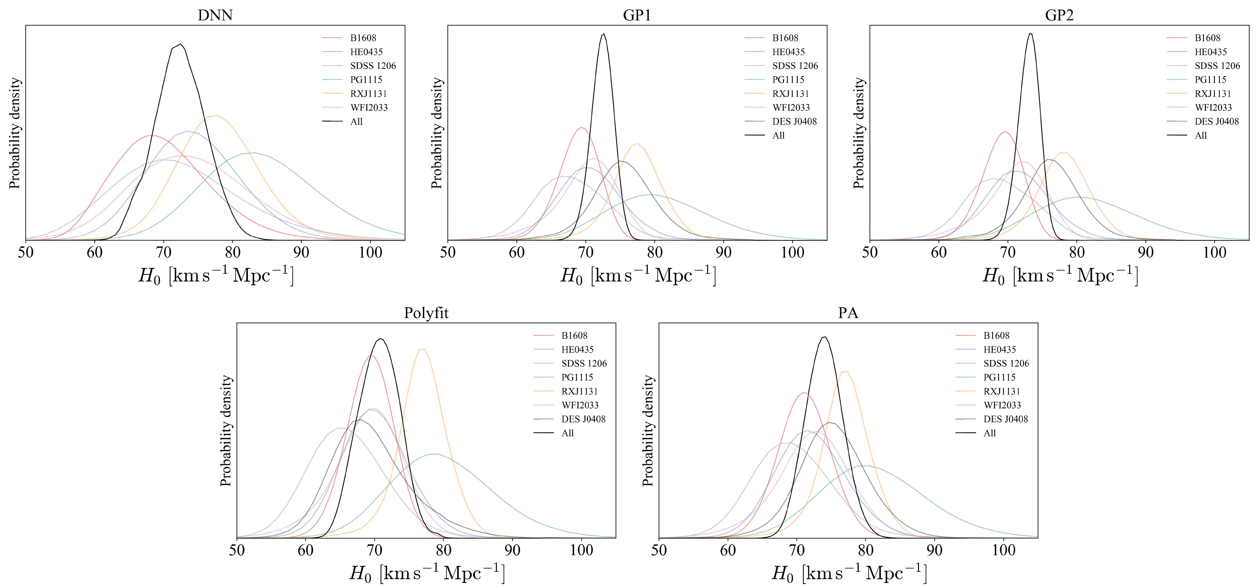

Figure 3.  (color online) Posterior PDFs of $ H_0 $ for the reconstructions constrained using all SGL systems and individual systems.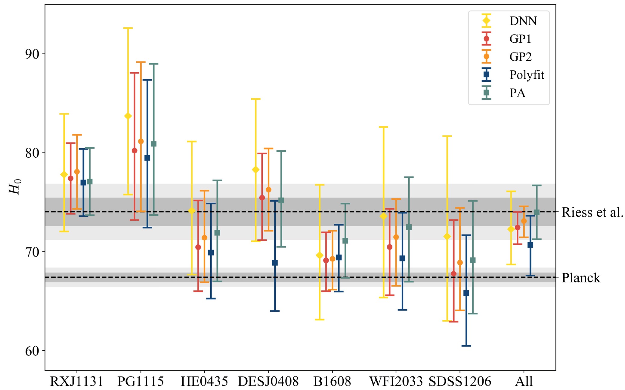

Figure 4.  (color online) Constraints on $ H_0 $ from individual systems using the different reconstruction methods compared with results from Planck Collaboration [9] and Riess et al. [13] including their respective 1σ and 2σ confidence intervals.

The values of $ H_0 $ derived from individual systems exhibit variability across both reconstruction methods and systems, underscoring the sensitivity of the results to the choice of methodology and the specific characteristics of the data. As illustrated in Fig. 4, the results based on the DNN reconstruction generally favor higher $ H_0 $ values, often aligning more closely with those of Riess et al.. The GP method yields narrower error bars, while the polyfit method produces slightly lower central values with intermediate uncertainties, consistent with trends observed in the combined system analysis. Although the result from the PG1115+080 system is marginally higher, the overall findings suggest a potential decrease in$ H_0 $with increasing lens redshift$ z_l $. However, this observation requires further investigation to robustly establish the influence of SGL characteristics on the determination of $ H_0 $.

The Hubble constant $ H_0 $ is a pivotal cosmological parameter representing the current expansion rate of the universe. Persistent discrepancies in its determination — specifically between values inferred from the CMB observations by the Planck Collaboration and those derived from the Cepheid distance ladder — pose a significant challenge to the standard ΛCDM model. This inconsistency, commonly referred to as the ''$ H_0 $ tension'', underscores the necessity for independent and precise measurements of $ H_0 $. Strong gravitational lensing (SGL) with time-delay measurements offers a promising avenue for addressing this issue, given its direct dependence on $ H_0 $. The H0LiCOW project has advanced this approach, recently providing the constraint $ H_0 = 73.3^{+1.7}_{-1.8} $ km s⁻¹ Mpc⁻¹ using six lensing systems. Within a new sample of seven SGL systems, six of which are drawn from the H0LiCOW dataset, the TDCOSMO collaboration determined the$ H_0 $ with an improved precision of 2.2% in a flat ΛCDM cosmology. However, these results are sensitive to the underlying cosmological model. Model-independent techniques, such as Gaussian process (GP) regression and polynomial fitting (polyfit), have also been employed to reconstruct distance-redshift relations and infer $ H_0 $, yielding consistent yet slightly varying results. Meanwhile, DL methods, leveraging DNNs trained on observational data, have emerged as powerful tools for curve reconstruction.

In this study, we applied model-independent methods — namely, DNN, GP, polyfit and Padé approximant (PA) — to reconstruct unanchored luminosity distances from the Pantheon+supernova dataset. These reconstructions were then combined with time-delay distance measurements from the TDCOSMO sample to constrain $ H_0 $, enabling an assessment of how reconstruction techniques influence the results. For all seven SGL systems, $ H_0 $ was constrained to $ H_0 = 72.3^{+3.8}_{-3.6} $ km s⁻¹ Mpc⁻¹, $ H_0 = 72.4^{+1.6}_{-1.7} $ km s⁻¹ Mpc⁻¹, $ H_0 = 73.1^{+1.5}_{-1.6} $ km s⁻¹Mpc⁻¹, $ H_0 = 70.7^{+3.0}_{-3.1} $ km s⁻¹ Mpc⁻¹ and $ H_0 = 74.0^{+2.7}_{-2.7} $ km s⁻¹ Mpc⁻¹ using the DNN, GP1 (squared-exponential function), GP2 (Matern function) polyfit, and PA methods, respectively. These results are consistent at the 1σ level and favor a higher value of $ H_0 $ compared to the Planck Collaboration's findings. Notably, the uncertainty in the DNN-derived $ H_0 $ is approximately twice as large as that obtained using the GP method, a phenomenon consistent with the findings of Qi et al. [39], reflecting the inherent differences in these methodologies. On a system-by-system basis, a potential trend emerges, suggesting that $ H_0 $ decreases with increasing lens redshift $ z_l $. This trend, previously noted by Liao et al. [35], warrants additional scrutiny to conclusively ascertain the impact of SGL characteristics on the determination of $ H_0 $.

Among these methods, DNN, GP, and PA exhibit greater flexibility than the polyfit approach. The DNN method excels at capturing local features of the observational data, whereas the GP method emphasizes global characteristics. Although the performance of the PA method surpasses that of polyfit, it still relies on a parameterized polynomial form, similar to the polyfit method. In uncertainty estimation, the GP method generally yields smaller uncertainties within the range of the observational data, while the DNN provides more reliable predictions beyond this range [37, 38]. This advantage positions the DNN method as a valuable tool for probing $ H_0 $ at higher redshifts. For instance, Li et al. [49] demonstrated this potential by combining mock SNe Ia samples with strongly lensed quasars, achieving a maximum redshift of 3.229, exceeding the redshift range of the Pantheon+ sample. Looking ahead, the Large Synoptic Survey Telescope (LSST) is anticipated to discover over 8000 lensed quasars, with approximately 3000 expected to have precisely measured time delays. These systems, reaching redshifts as high as 5 [50], present an unprecedented opportunity to address the Hubble tension. DNN-based reconstructions will likely play a pivotal role in combining observed SGL and SNe Ia data to refine our understanding of $ H_0 $ and the underlying cosmological model.