Data taking strategy for ${\boldsymbol\psi \bf (3770)} $ and ${\boldsymbol\Upsilon{ \bf (4}{\boldsymbol S})} $ branching fraction measurements at e⁺e⁻ colliders

The $ \psi(3770) $ state above the $ D\bar{D} $ threshold and the $ \Upsilon(4S) $ state above the $ B\bar{B} $ threshold are two typical broad resonances. Their dominant decay modes are open-flavor meson pair final states and hadronic or radiative transitions to low lying quarkonia. Their decays into light hadronic ($ {\text{non}-}{D}\bar{D} $, $ {\text{non}-}B\bar{B} $) final states are suppressed according to the OZI rule [1−3]. Most of these studies were performed using $ e^+e^- $ collision experiments, and the total cross sections of the resonance production and continuum process were of the same order of magnitude. In this case, the interference between the continuum and resonance amplitudes might be large and cannot be ignored. The mishandling of the interference effect will lead to a systematic bias with a much larger size compared with the statistical uncertainty and comparable to or even larger than all the other sources of systematic uncertainties [4]. The optimal solution to this problem is to take data with a strategy of accumulating data at the resonance peak and energy points off the peak (called continuum data).

The BESIII and Belle II are $ e^+e^- $ collision experiments that operate in the charmonium and bottomonium energy regions. At the BESIII experiment, $ 20\; {\rm{fb}}^{-1} $ data were accumulated by 2024 at the center-of-mass energy of $ \sqrt{s} = 3.773\; {\rm{GeV}} $, which is the peak position of the $ \psi(3770) $ state [5]. This data sample is at least six times larger than the one collected by BESIII up to 2019 and dozens of times larger than those in the CLEOc and BESII measurements [6]. The Belle II experiment plans to capture about $ 50\; {\rm{ab}}^{-1} $ data at the peak position of the $ \Upsilon(4S) $ ($ \sqrt{s} = 10.58\; {\rm{GeV}} $) state [7], which are $ 10^2 $ ($ 10^3 $) of times larger than the data samples of the Belle and BaBar (CLEO) experiments [6]. With the currently available BESIII and expected Belle II data samples, the precision of the branching fraction of $ \psi(3770)\to{\text{non}-}{D}\bar{D} $ and $ \Upsilon(4S)\to{\text{non}-}B\bar{B} $ decays can be improved significantly. Therefore, determining an optimal data taking strategy is essential.

This work focuses on the relative uncertainties of the branching fractions of $ \psi(3770)\to{\text{non}-}{D}\bar{D} $ and $ \Upsilon(4S)\to {\text{non}-}B\bar{B} $ decays. We take the optimization of $ \psi(3770)/ \Upsilon(4S) \to \eta^{\prime}\phi $ measurement as an example. Monte Carlo (MC) simulation and Fisher information methods were employed to simulate various data taking cases with two parameters: the branching fraction of $ {\text{non}-}{D}\bar{D} $ or $ {\text{non}-} B\bar{B} $ decays denoted as $ {\cal{B}} $, and the relative angle between resonance and continuum amplitudes denoted as ϕ. The optimal data taking scheme obtained from both methods is consistent. Herein, to achieve the measurements of branching fractions of $ \psi(3770)\to{\text{non}-}{D}\bar{D} $ and $ \Upsilon(4S)\to {\text{non}-}B\bar{B} $ decays, we aim to determine the following:

● What are the optimal $ \sqrt{s} $ values for data taking around the resonances?

● How many energy points around an optimal $ \sqrt{s} $ are necessary for the scan?

● What are the required data sizes to achieve a specific precision in the branching fraction measurements?

Within a specified period of data taking time or equivalently for a given integrated luminosity, we attempt to determine the scheme that can provide the best precision for branching fraction measurements of $\psi(3770)\to {\text{non}-}{D}\bar{D}$ or $ \Upsilon(4S)\to{\text{non}-}B\bar{B} $ decays. The sampling technique is utilized to simulate various data taking strategies, among which the optimal one will be selected. For specific simulations, the likelihood function is constructed as

where $ x_i $ and $ x_{i}^{\rm{exp}} $ are the numbers of observed and expected events, respectively, of $ \psi(3770)\to{\text{non}-}{D}\bar{D} $ or $ \Upsilon(4S)\to{\text{non}-}B\bar{B} $ decays, the subscript i labels the i-th scan energy point, and $ N_{\rm pt} $ is the number of energy points. For a certain exclusive final state f, the $ x_{i}^{\rm{exp}} $ in a data sample taken at the i-th energy point with an integrated luminosity of $ {\cal{L}}_i $ is given by

where ϵ is the selection efficiency of signal reconstruction, and $ \sigma_{\rm{exp}} $, with $ {\cal{B}} $ and ϕ as two parameters, is the expected cross section at $ \sqrt{s} $. The maximum value of $ {\cal{B}} $, derived from a conservative estimate of the summed branching ratios for the resonance decaying to light hadronic final states as reported by the Particle Data Group (PDG) [6], is $ 1 \times 10^{-3} $ for $ \psi(3770)\to{\text{non}-}{D}\bar{D} $ decays and $ 1 \times 10^{-6} $ for $ \Upsilon(4S)\to{\text{non}-}B\bar{B} $ decays. The cross section $ \sigma_{\rm{exp}} $ can be expressed as

where $ a_c^{f}(\sqrt{s}) $ is the continuum amplitude of $ e^+e^- \to f $, and $ a_{R}^{f}(\sqrt{s}) $ is the resonance amplitude of $ e^+e^- \to\; R \to f $. They are parametrized as

where $ PS(\sqrt{s}) $ is the phase space factor at $ \sqrt{s} $. In the continuum amplitude, the constants a and n describe the magnitude and slope of the continuum process, respectively. In the Breit-Wigner function for the resonance amplitude, M, Γ, and $ \Gamma_{ e^+e^-} $ are the mass, total width, and partial width to $ e^+e^- $ final state of the resonance R, respectively. For the $ \eta^\prime \phi $ final state, the phase space factor is $PS(\sqrt{s}) = \; q^3(\sqrt{s})/s$, where $ q(\sqrt{s}) $ is the momentum of $ \eta^\prime $ or ϕ. The following study focused on the optimization of statistical uncertainty. The values of the key parameters for the numerical calculations presented in the following sections are summarized in Table 1. In the fitting procedure, $ {\cal{B}} $ and ϕ are defined as two free parameters to fit $ \sigma_{\rm{exp}}(\sqrt{s}) $. The maximization of the likelihood function $ LF $ presented in Eq. (1) yields the optimal estimate for $ {\cal{B}} $.

Parameter	$ \psi(3770)\to{\text{non}-} D \bar{D} $	$ \Upsilon(4S)\to{\text{non}-}B\bar{B} $
$ M $/(${ {\rm{GeV} } }/c^2$)	3.7736 [6]	10.58 [6]
$ \Gamma_{ e^+e^-} $/$ {\rm{keV}} $	0.26 [6]	0.28 [6]
$ \Gamma $/$ {\rm{MeV}} $	27.2 [6]	20.5 [6]
$ \star {\cal{B}} $	free	free
$ \star\phi $	free	free
ϵ	10% [8−12]	15% [8−12]
a	1.82 [8−12]	$ 3.2\times10^{-2.5} $ [8−12]
n	5.82 [8−12]	3.00 [8−12]

Table 1.  Values of key parameters for the numerical calculation. The quantities with $\star $ are set as free parameters, and the others are fixed for the corresponding study.

In the following analysis, we assume that the value of $ {\cal{B}} $ is known. Under this assumption, we aim to address the questions posed at the end of Sec. I. However, upon further reflection on the first two questions, we notice that they are interconnected. Specifically, the optimal number of energy points depends on the distribution of points, and vice versa. To resolve this dilemma, we begin with a simple distribution to determine the optimal number of energy points, enabling us to finalize the total number of energy points required.

We take $N_{\rm pt} = 100$ energy points and $N_{\rm br} = 300$ branching fractions as a tentative beginning. The values of energies and branching fractions are calculated via

where the first energy point is $ E_{\rm{c.m.}}^0 = 3.74\; {\rm{GeV}} $ with a branching fraction of $ {\cal{B}}_0 = 1\times 10^{-6} $, and the last energy point is $ E_{\rm{c.m.}}^f = 3.80\; {\rm{GeV}} $ with a branching fraction of $ {\cal{B}}_f = 1\times 10^{-3} $ for $ \psi(3770) $ decays. Correspondingly, for $ \Upsilon(4S) $ decays, $ E_{\rm{c.m.}}^0 = 10.56\; {\rm{GeV}} $, $ {\cal{B}}_0 = 1\times 10^{-9} $, $ E_{\rm{c.m.}}^f = 10.60 \; {\rm{GeV}} $, and $ {\cal{B}}_f = 1\times 10^{-6} $. The energy interval and branching fraction interval are calculated with $ \delta E_{\rm{c.m.}} = ( E_{\rm{c.m.}}^f - E_{\rm{c.m.}}^0)/ N_{\rm{pt}} $ and $ \delta {\cal{B}} = ( {\cal{B}}_f - {\cal{B}}_0)/ N_{\rm{br}} $.

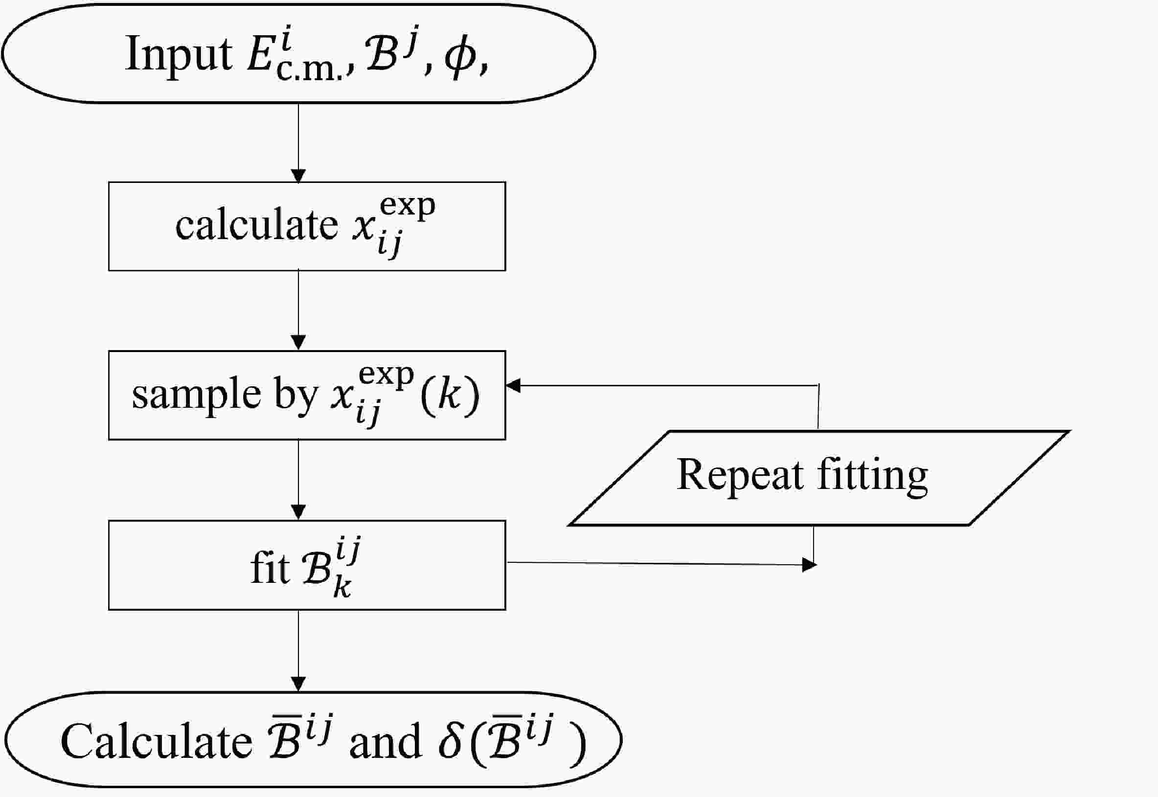
To reduce the statistical fluctuation, we repeat sampling $ N_{\rm{samp}} = 200 $ times for each scheme of an $ E_{\rm{c.m.}}^i $ and $ {\cal{B}} $ combination, which satisfy a Gaussian distribution with a mean of $ x_{i}^{\rm{exp}} $ and deviation of $ \sqrt{ x_{i}^{\rm{exp}}} $. The general flowchart of sampling and fitting is presented in Fig. 1. We obtain the mean value of $ {\cal{B}}^{ij}_k $ and its error $ \delta( {\cal{B}}^{ij}_k) $ from fitting to the k-th sample. The average value of $ {\cal{B}} $ and the corresponding uncertainty from fitting to the 200 samples are calculated via [13]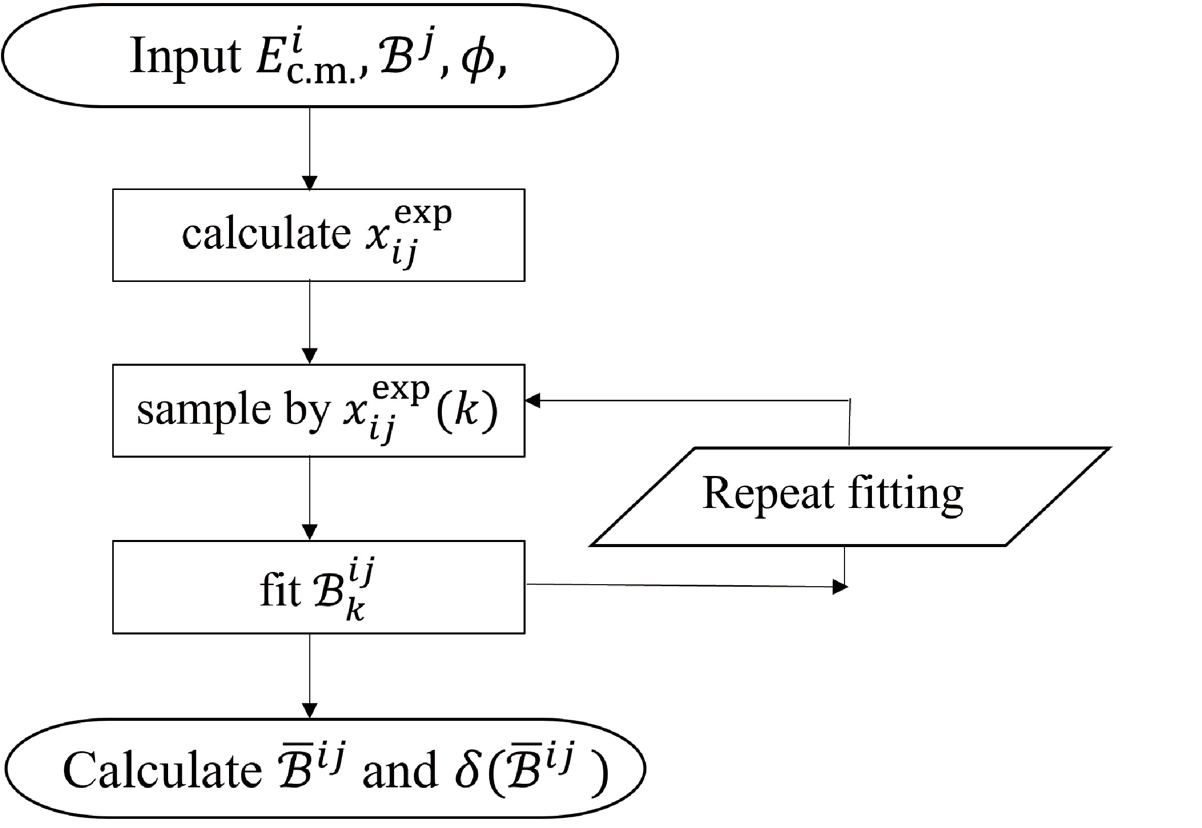

Figure 1.  Flowchart of the sampling, where $ ij $ ($i = 1,2,\cdots, N_{\rm{pt}}$; $j = 1,2,\cdots, N_{\rm{br}}$) denotes a specific scheme of an $ E_{\rm{c.m.}}^i $ and $ {\cal{B}} $ combination, and $ k $ ($k = 1,2,\cdots, N_{\rm{samp}}$) represents the $ k $-th sampling time.

The average relative uncertainty is calculated via

Here, note that $ ij $ denotes a specific scheme of an $ E_{\rm{c.m.}}^i $ and $ {\cal{B}} $ combination. Additionally, k represents the k-th sampling time. $ \bar{B}^{ij} $ and $ \delta(\bar{B}^{ij}) $ represent the average value and error of the branching fraction from the fit, respectively. Without the special declaration, the meaning of the average defined by Eqs. (8) and (9) is maintained in the following analysis.

According to the available data at the BESIII experiment and future data acquisition strategies of the Belle II experiment, the integrated luminosities of the data we use are $ 20\; {\rm{fb}}^{-1} $ at $ \sqrt{s} = 3.773\; {\rm{GeV}} $ and $ 50\; {\rm{ab}}^{-1} $ at $ \sqrt{s} = 10.58\; {\rm{GeV}} $, respectively. $ {\cal{B}} $ and ϕ as free parameters in the fits, and we obtain the results for each $ 30^{\circ} $ variations in the phase angle, as presented in Fig. 2 for $ \psi(3770) $ decays and Fig. 3 for $ \Upsilon(4S) $ decays. The colors represent the $ E( {\cal{B}}) $ for each energy point and branching fraction combination at the corresponding phase angle ϕ.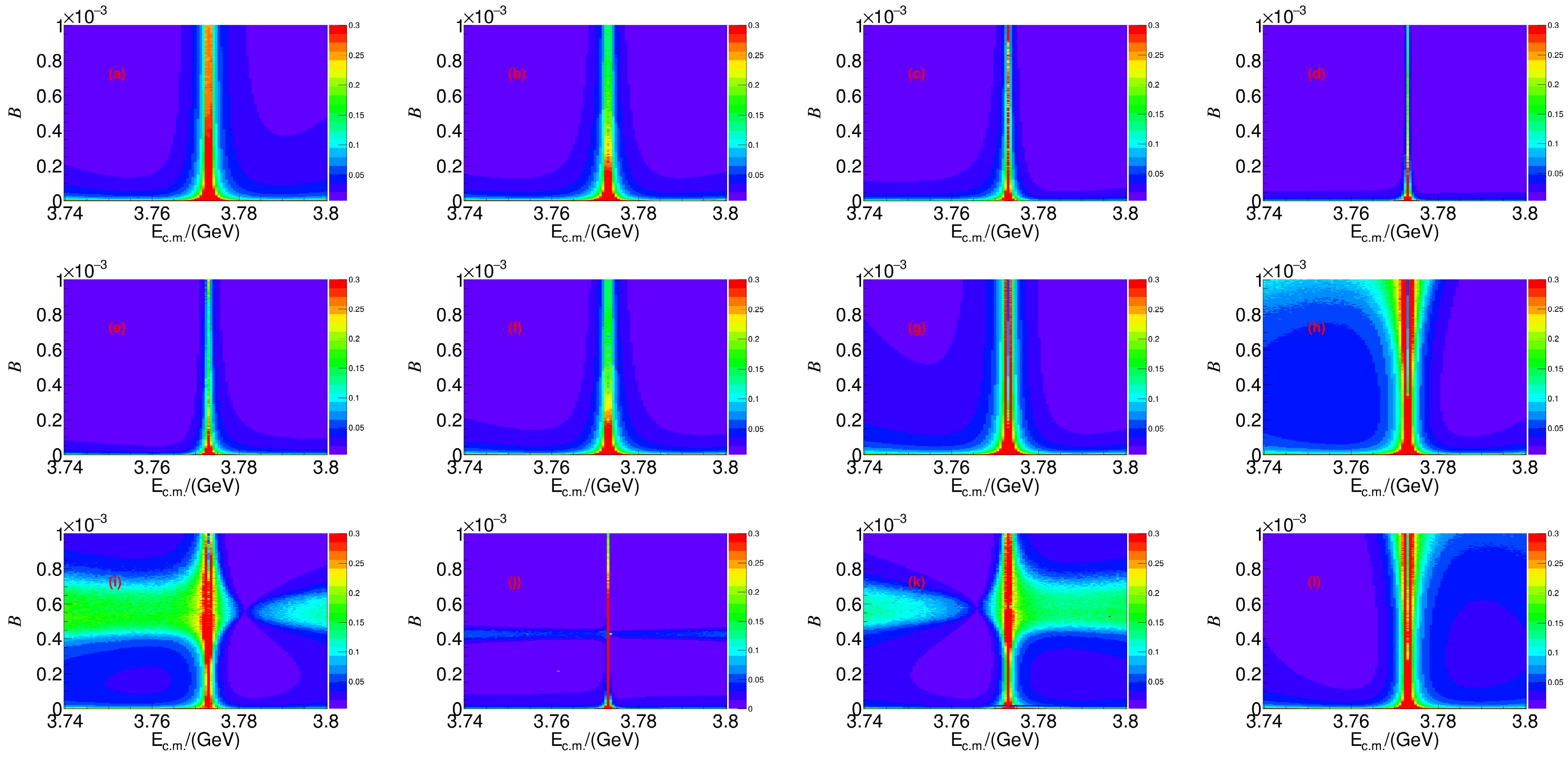

Figure 2.  (color online) Distributions of $ E( {\cal{B}}) $ with $ E_{\rm{c.m.}}^i $ and the branching fraction for $ \psi(3770)\to{\text{non}-}D\bar{D} $ decays with different phase angles ϕ: (a) $ 0^\circ $, (b) $ 30^\circ $, (c) $ 60^\circ $, (d) $ 90^\circ $, (e) $ 120^\circ $, (f) $ 150^\circ $, (g) $ 180^\circ $, (h) $ 210^\circ $, (i) $ 240^\circ $, (j) $ 270^\circ $, (k) $ 300^\circ $, and (l) $ 330^\circ $.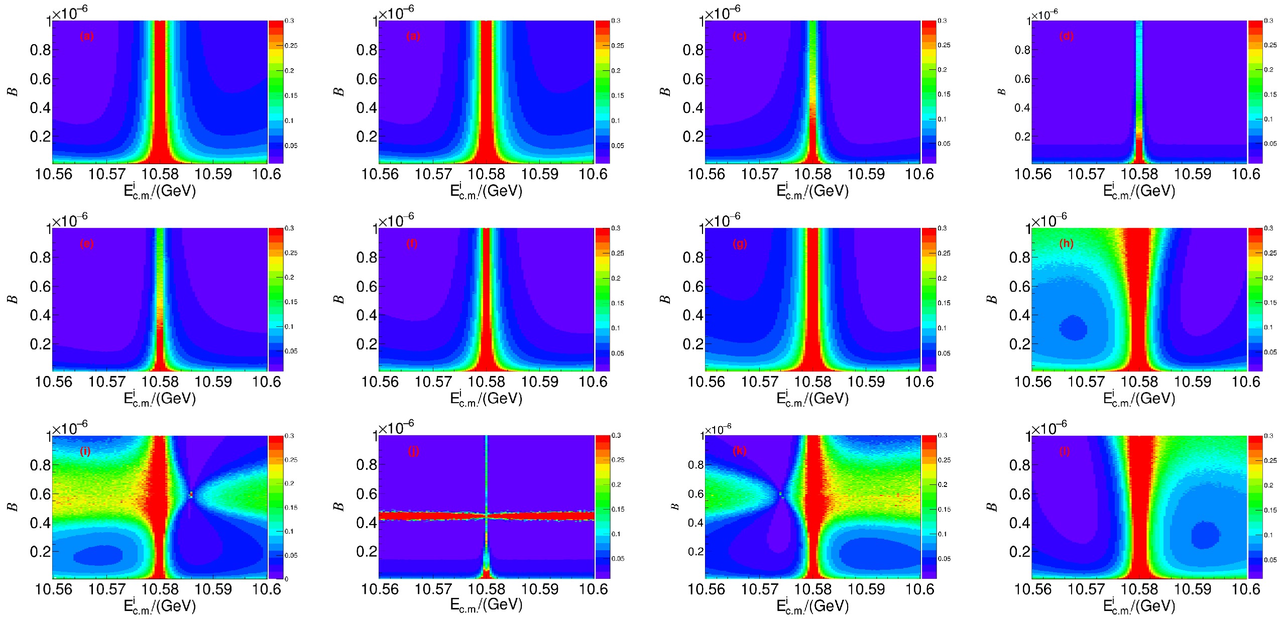

Figure 3.  (color online) Distributions of $ E( {\cal{B}}) $ with $ E_{\rm{c.m.}}^i $ and the branching fraction for $ \Upsilon(4S)\to{\text{non}-}B\bar{B} $ decays with different phase angles ϕ: (a) $ 0^\circ $, (b) $ 30^\circ $, (c) $ 60^\circ $, (d) $ 90^\circ $, (e) $ 120^\circ $, (f) $ 150^\circ $, (g) $ 180^\circ $, (h) $ 210^\circ $, (i) $ 240^\circ $, (j) $ 270^\circ $, (k) $ 300^\circ $, and (l) $ 330^\circ $.

In mathematical statistics, Fisher information quantifies the amount of information that a random variable X carries about a known parameter θ [14]. In the context of our study, Fisher information is employed to estimate the parameter $ \theta = ( {\cal{B}}, \phi) $ based on the observed event numbers $ \boldsymbol{x} = (x_1, x_2) $ as described in Sec. II.A.

According to Eq. (1), the score function is constructed as

and the Fisher information matrix is defined as the covariance matrix of the score function. Concretely,

where $ E_\theta $ represents the expected value of the outer product of the score function $s(\theta,\boldsymbol{x}) s(\theta,\boldsymbol{x})^{\rm{T}}$ given the parameter θ. When considering $ {\cal{B}} $ and ϕ as two free parameters, the Fisher information matrix of $ \theta = ( {\cal{B}}, \phi) $ is a $ 2 \times 2 $ matrix, and its elements are

where indices 1 and 2 indicate $ {\cal{B}} $ and ϕ, respectively. Inverting the $ 2 \times 2 $ matrix yields the asymptotic covariance matrix:

Hence, the variance of the branching fraction can be determined as

where $ x_{1}^{\rm{exp}} $ and $ x_2^{\rm{exp}} $ are the expected events at energy points $ E_{\rm{c.m.}}^{i} $ and the resonance, respectively. $ DB_i $ and $ D\phi_i $ denote $ \partial x_i^{\rm{exp}}/\partial {\cal{B}} $ and $ \partial x_i^{\rm{exp}}/\partial \phi $, respectively. As in Sec. II, we present $ E( {\cal{B}}) $ using Fisher information. The same phase ϕ distributions are shown in Figs. 4 and 5. The results are consistent with the methodology employed in the MC simulation.

Figure 4.  (color online) Distributions of $ E( {\cal{B}}) $ with $ E_{\rm{c.m.}}^i $ and the branching fraction obtained by Fisher information for $ \psi(3770)\to{\text{non}-} D\bar{D} $ decays with different phase angles ϕ: (a) $ 0^\circ $, (b) $ 30^\circ $, (c) $ 60^\circ $, (d) $ 90^\circ $, (e) $ 120^\circ $, (f) $ 150^\circ $, (g) $ 180^\circ $, (h) $ 210^\circ $, (i) $ 240^\circ $, (j) $ 270^\circ $, (k) $ 300^\circ $, and (l) $ 330^\circ $.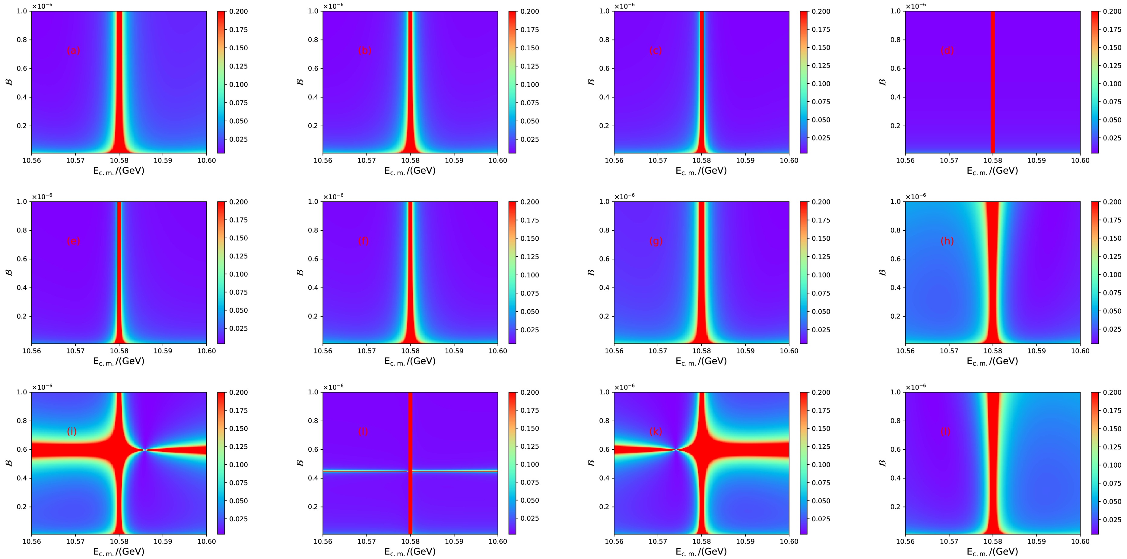

Figure 5.  (color online) Distributions of $ E( {\cal{B}}) $ with $ E_{\rm{c.m.}}^i $ and the branching fraction obtained by Fisher information for $ \Upsilon(4S)\to{\text{non}-}B\bar{B} $ decays with different phase angles ϕ: (a) $ 0^\circ $, (b) $ 30^\circ $, (c) $ 60^\circ $, (d) $ 90^\circ $, (e) $ 120^\circ $, (f) $ 150^\circ $, (g) $ 180^\circ $, (h) $ 210^\circ $, (i) $ 240^\circ $, (j) $ 270^\circ $, (k) $ 300^\circ $, and (l) $ 330^\circ $.

Drawing from previous studies, a critical question emerges: Where should the optimal energy point be? In addressing this inquiry, Ref. [15] indicates that the relative phase ϕ is approximately $ 270^{\circ} $. Accordingly, Figs. 6 and 7 present the fitting results for ϕ ranging from $ 240^\circ $ to $ 300^\circ $ in $ 10^{\circ} $ increments. The red line in each plot represents the optimal energy point corresponding to the best precision of $ E( {\cal{B}}) $ as determined using the branching fraction. For the phase angles ranging from $ 240^{\circ} $ to $ 300^{\circ} $, the optimal energy points are projected onto the $ E_{\rm{c.m.}}^i $ axis, as shown in Fig. 8. This figure shows that the optimal energy points for $ \psi(3770)\to{\text{non}-}{D}\bar{D} $ decays are $ 3.769 \; {\rm{GeV}} $ and $ 3.781\; {\rm{GeV}} $, whereas those for $ \Upsilon(4S)\to{\text{non}-}B\bar{B} $ decays are $ 10.574\; {\rm{GeV}} $ and $ 10.585\; {\rm{GeV}} $. We should note that the optimal energies will differ if the phase ϕ is in different ranges.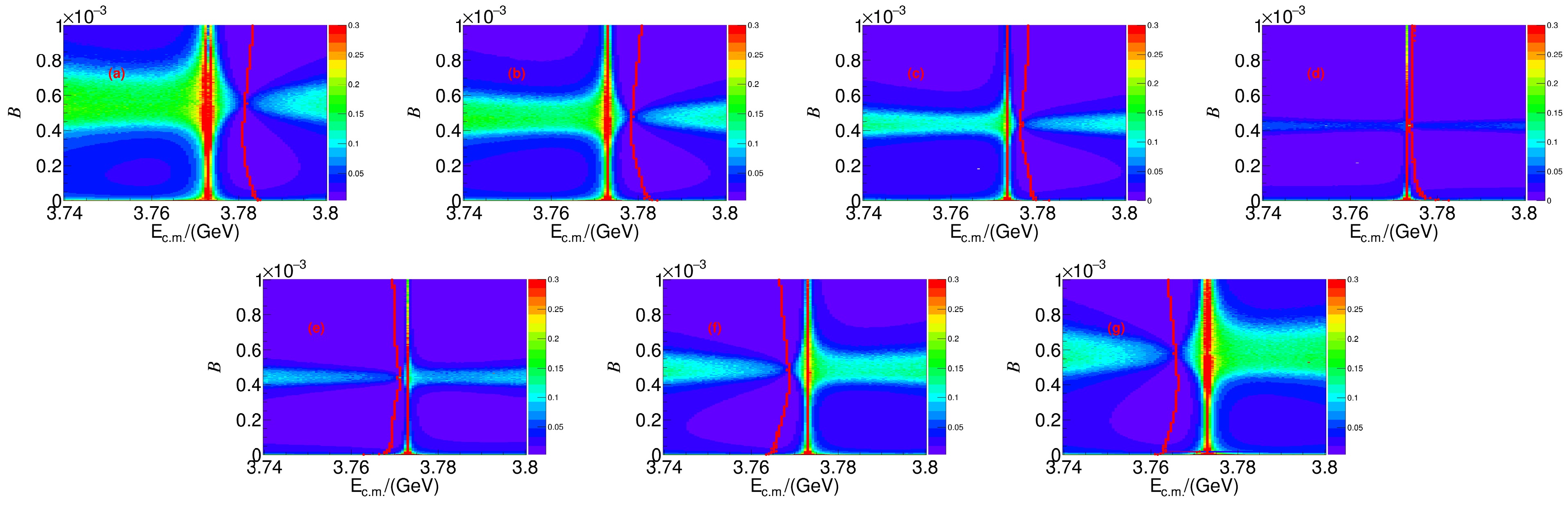

Figure 6.  (color online) Distributions of $ E( {\cal{B}}) $ with $ E_{\rm{c.m.}}^i $ and the branching fraction for $ \psi(3770)\to{\text{non}-} D\bar{D} $ decays from specific phase angles ϕ: (a) $ 240^\circ $, (b) $ 250^\circ $, (c) $ 260^\circ $, (d) $ 270^\circ $, (e) $ 280^\circ $, (f) $ 290^\circ $, and (g) $ 300^\circ $. The red lines show the best precision of $ E( {\cal{B}}) $ versus the branching ratio $ {\cal{B}} $.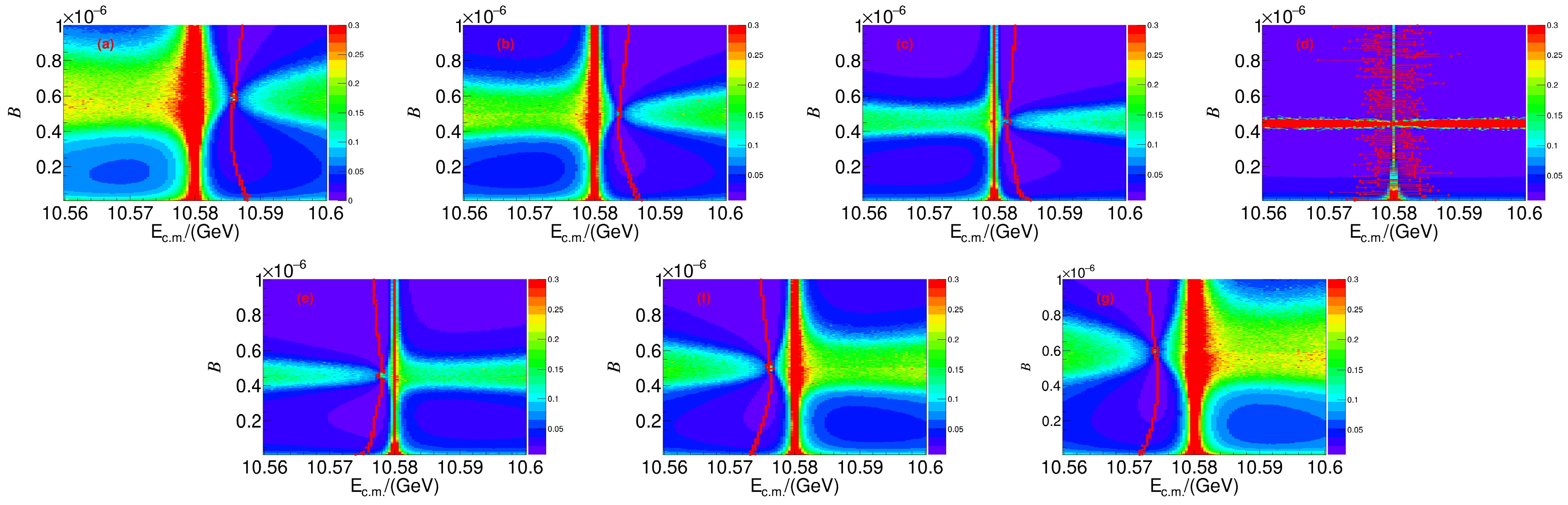

Figure 7.  (color online) Distributions of $ E( {\cal{B}}) $ with $ E_{\rm{c.m.}}^i $ and the branching fraction for $ \Upsilon(4S)\to{\text{non}-}B\bar{B} $ decays from specific phase angles ϕ: (a) $ 240^\circ $, (b) $ 250^\circ $, (c) $ 260^\circ $, (d) $ 270^\circ $, (e) $ 280^\circ $, (f) $ 290^\circ $, and (g) $ 300^\circ $. The red lines show the best precision of $ E( {\cal{B}}) $ versus the branching ratio $ {\cal{B}} $.

Figure 8.  (color online) Distribution of optimal energy points projected onto the $ E_{\rm{c.m.}}^{i} $ axis from specific phase angle ϕ ranging from $ 240^\circ $ to $ 300^\circ $ for (a) $ \psi(3770) $ decays and (b) $ \Upsilon(4S) $ decays.

The last question is the relationship between the integrated luminosity and the precision of branching fraction measurements. For the fitting procedure involving branching fractions that span several orders of magnitude, we assume an equal allocation of integrated luminosity between the low-energy ($ L_{\rm{low}} $) and high-energy ($ L_{\rm{high}} $) data acquisition points. The results of the integrated luminosity optimization for $ \psi(3770) $ are shown in Fig. 9, where seven curves represent different relative phases ($ \phi = 240^{\circ}, \; 250^{\circ}, \; 260^{\circ}, \; 270^{\circ}, \; 280^{\circ}, \; 290^{\circ}, \; 300^{\circ} $). Similarly, Fig. 10 illustrates a corresponding integrated luminosity optimization scheme for $ \Upsilon(4S) $. Table 2 summarizes the integrated luminosity requirements for an effective data acquisition strategy aimed at achieving a projected 10% precision of $ E( {\cal{B}}) $ at both energy points. The research results indicate that, when considering the maximum value of $ {\cal{B}} $ based on conservative estimates, a minimum integrated luminosity of $ 500\; {\rm{pb}}^{-1} $ is required for $ \psi(3770) $ decays, whereas $ 200\; {\rm{fb}}^{-1} $ is necessary for $ \Upsilon(4S) $ decays.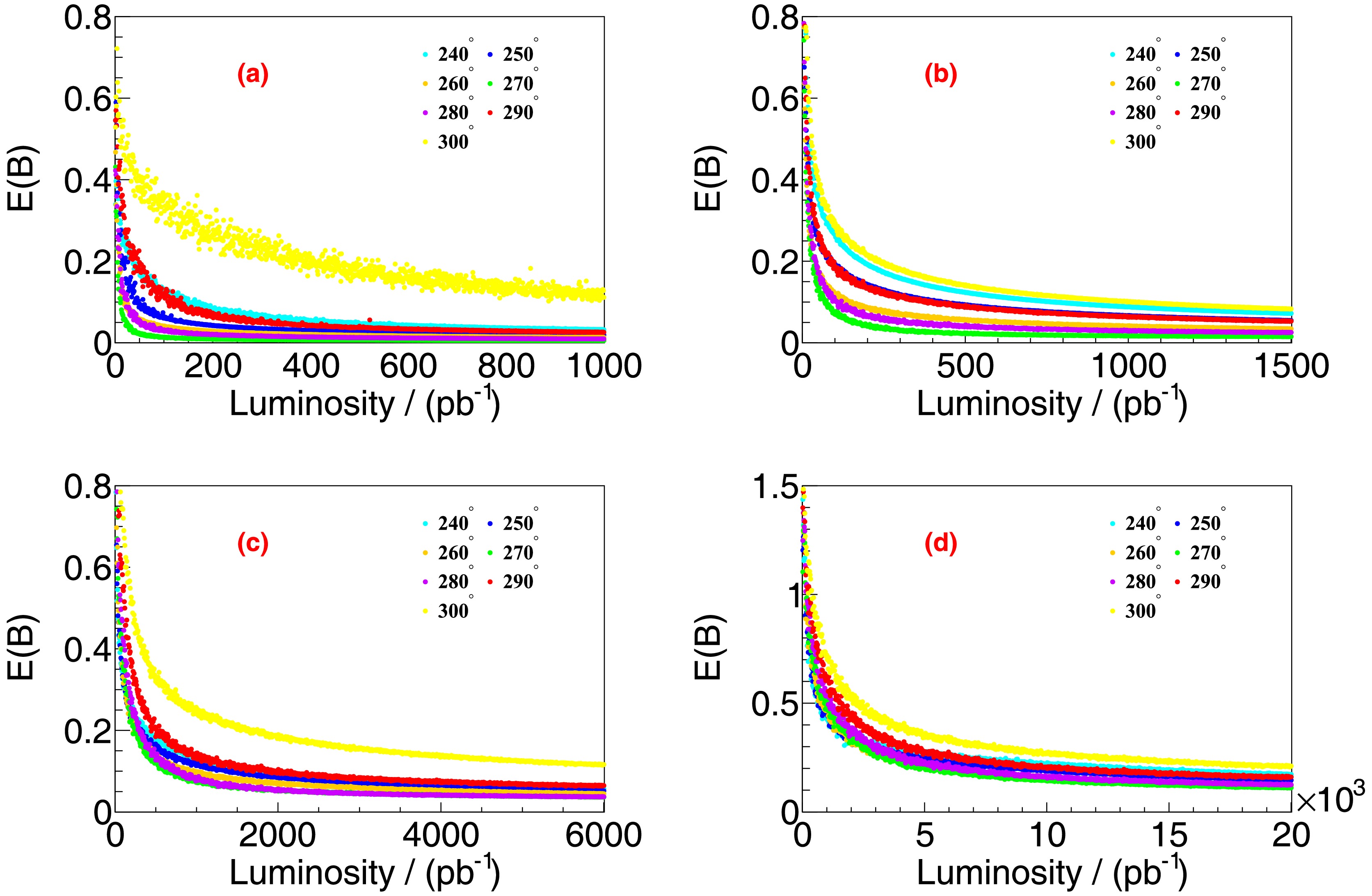

Figure 9.  (color online) Distributions of $ E( {\cal{B}}) $ with the integrated luminosity of data sample for $ \psi(3770)\to{\text{non}-} D\bar{D} $ decays with branching fractions of (a) $ 1 \times 10^{-3} $, (b) $ 1\times10^{-4} $, (c) $ 1\times 10^{-5} $, and (d) $ 1\times10^{-6} $.

Figure 10.  (color online) Distributions of $ E( {\cal{B}}) $ with the integrated luminosity of data sample for $ \Upsilon(4S)\to{\text{non}-}B\bar{B} $ decays with branching fractions of (a) $ 1 \times 10^{-6} $, (b) $ 1 \times 10^{-7} $, and (c) $ 1\times 10^{-8} $.

$ {\cal{B}} $	$ \psi(3770)\to{\text{non}-} D\bar{D} $	$ {\cal{B}} $	$ \Upsilon(4S)\to{\text{non}-}B\bar{B} $
$ 1\times10^{-3} $	$ 500 \;{\rm{pb}}^{-1} $	$ 1\times10^{-6} $	$ 200 \;{\rm{fb}}^{-1} $
$ 1\times10^{-4} $	$ 800 \;{\rm{pb}}^{-1} $	$ 1\times10^{-7} $	$ 800 \;{\rm{fb}}^{-1} $
$ 1\times10^{-5} $	$ 3 \;{\rm{fb}}^{-1} $	$ 1\times10^{-8} $	$ 5 \;{\rm{ab}}^{-1} $
$ 1\times10^{-6} $	$ 14 \;{\rm{fb}}^{-1} $

Table 2.  Relationship between integrated luminosity and $ {\cal{B}} $ with $ E( {\cal{B}}) $ fixed to 10%.

Based on the findings presented in Sec. V.A, we initially assumed an integrated luminosity ratio of $ L_{\rm{low}} : L_{\rm{high}} = 1:1 $ without considering the effects of different integrated luminosities at different energy points. To achieve optimal precision in the branching fraction measurements, we vary the parameter ${X}_{i}\equiv {L}_{\rm{low}}/( {L}_{\rm{low}} + {L}_{\rm{high}})$ to determine the corresponding $ E( {\cal{B}}) $. The optimized $X_i$ values for both energy points related to $ \psi(3770) $ are shown in Fig. 11. Figure 12 illustrates a similar integrated luminosity optimization scheme for $ \Upsilon(4S) $. We assign equal weights to different phase angles corresponding to the same branching ratio, thereby achieving optimal results for that branching ratio. This is illustrated in Fig. 13, where the minimum value of $ E( {\cal{B}}) $ occurs at $X_i = 0$ for $ \psi(3770)\to{\text{non}-}{D}\bar{D} $ decays and $X_i= 0.5$ for $ \Upsilon(4S)\to {\text{non}-} B\bar{B} $ decays, which correspond to integrated luminosity ratios of $ L_{\rm{low}} : L_{\rm{high}} = 0:1 $ and $ 1:1 $, respectively.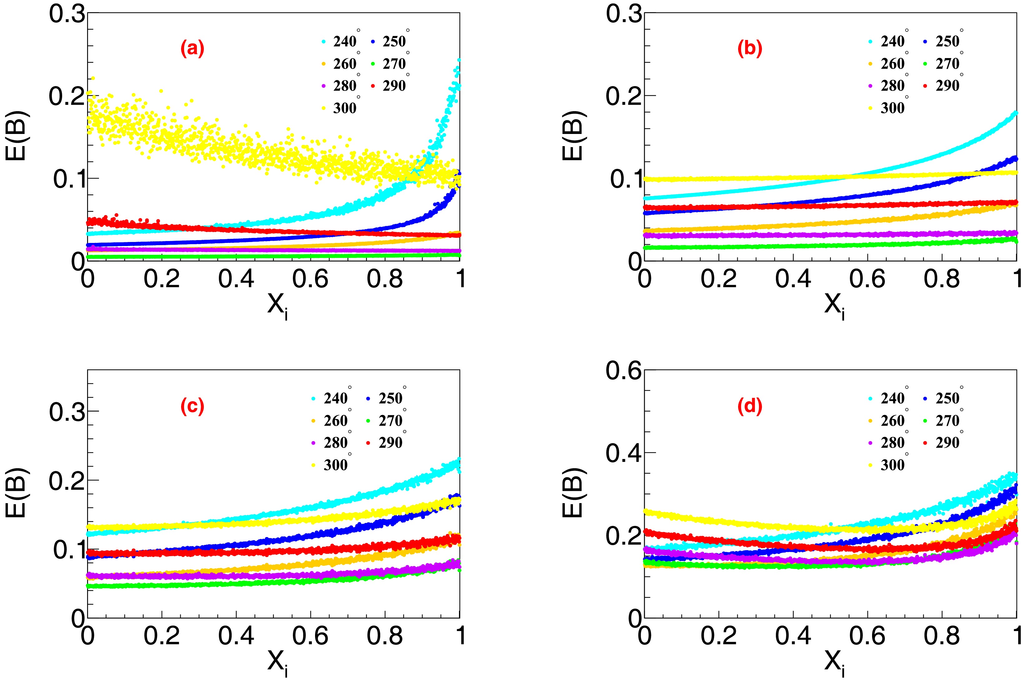

Figure 11.  (color online) Distributions of $ E( {\cal{B}}) $ with the integrated luminosity allocation ratio $ X_i $ for $ \psi(3770)\to{\text{non}-} D\bar{D} $ decays with branching fractions of (a) $ 1\times10^{-3} $, (b) $ 1\times10^{-4} $, (c) $ 1\times 10^{-5} $, and (d) $ 1\times10^{-6} $. The total luminosities and $ {\cal{B}} $s are fixed according to Table 2.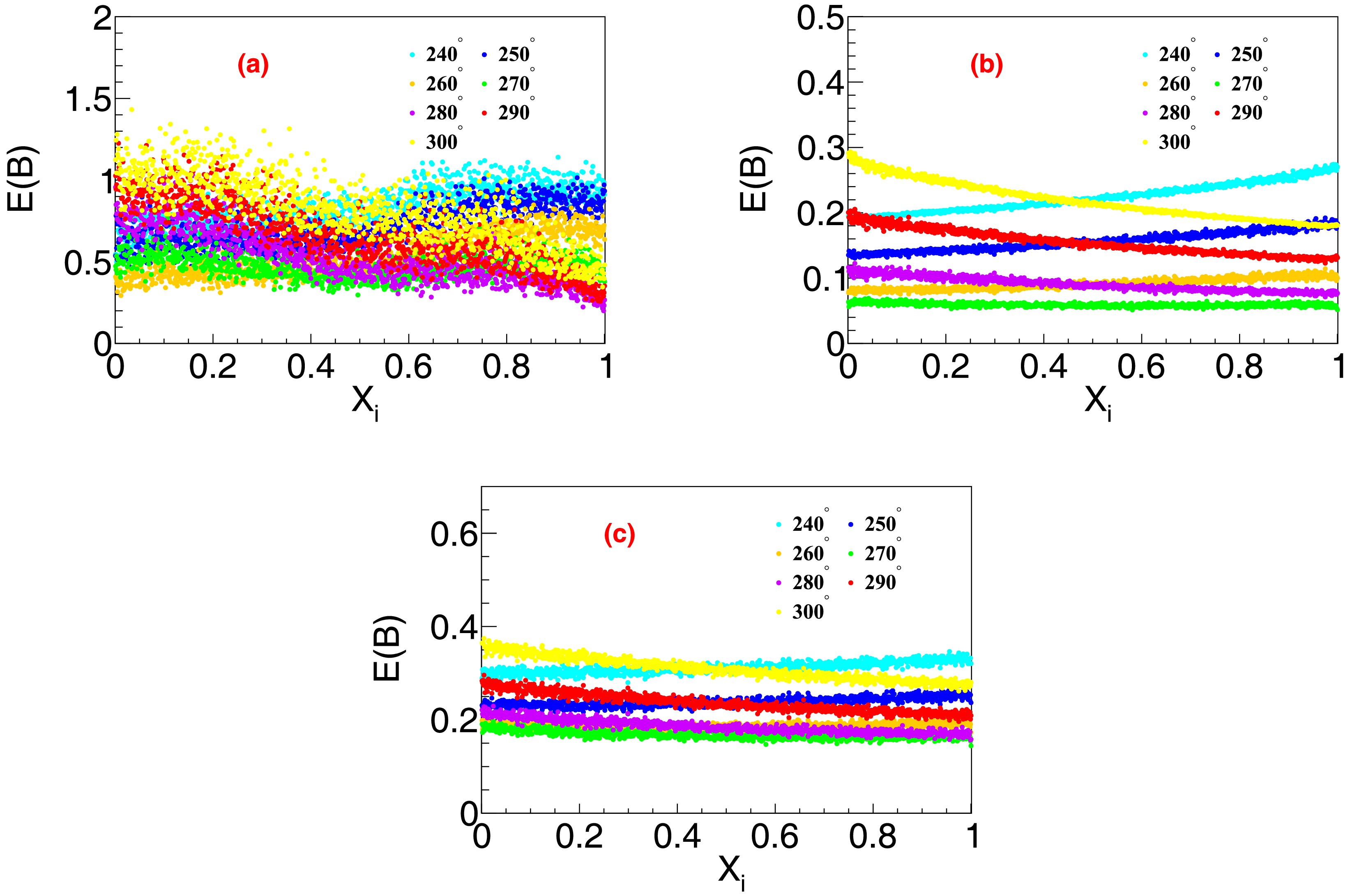

Figure 12.  (color online) Distributions of $ E( {\cal{B}}) $ with the integrated luminosity allocation ratio $ X_i $ for $ \Upsilon(4S)\to{\text{non}-}B\bar{B} $ decays with branching fractions of (a) $ 1\times10^{-6} $, (b) $ 1\times10^{-7} $, and (c) $ 1\times 10^{-8} $. The total integrated luminosities and $ {\cal{B}} $s are fixed according to Table 2.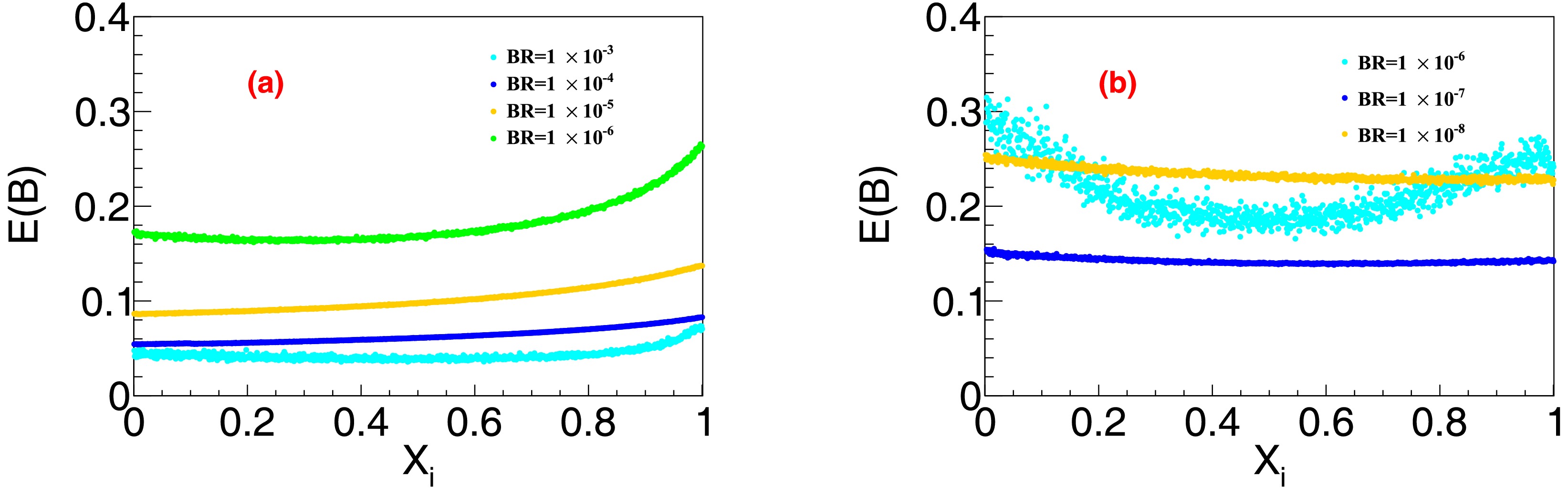

Figure 13.  (color online) Distributions of $ E( {\cal{B}}) $ with the integrated luminosity allocation ratio $ X_i $, obtained by assigning equal weights to different phase angles at the same branching ratio, for (a) $ \psi(3770)\to{\text{non}-} D\bar{D} $ decays and (b) $ \Upsilon(4S)\to{\text{non}-}B\bar{B} $ decays.

The minor deviations, either higher or lower than the continuum cross sections observed in Refs. [10, 16−19], may have indicated nonzero $ \psi(3770) $ decays into light hadron final states, and more data are required to confirm the observations. In the BESIII experiment, the peak luminosity is approximately $ 1 \times 10^{33}\; {\rm{cm}}^{-2} {\rm{s}}^{-1} $ at $ \sqrt{s} = $ 3.773 GeV. A data acquisition period of 12 days is expected to be sufficient to achieve a projected precision of 10% in the measurements of the $ \psi(3770)\to{\text{non}-}{D}\bar{D} $ branching fraction.

In June 2022, SuperKEKB, the asymmetric energy accelerator that provides $ e^+e^- $ collisions inside the Belle II detector, achieved a new luminosity record of $ 4.7 \times 10^{34}\; {\rm{cm}}^{-2} {\rm{s}}^{-1} $ and recorded $ 15\; {\rm{fb}}^{-1} $ data per week. SuperKEKB aims to achieve a luminosity higher than $ 1 \times 10^{35}\; {\rm{cm}}^{-2} {\rm{s}}^{-1} $ in the near future. This accomplishment enables measurements with a branching fraction uncertainty of 10% to be completed within two months. If this larger data sample is collected slightly above the $ \Upsilon(4S) $ peak, it will allow for the direct measurement of the $ B^{+} $ to $ B^{0} $ production ratio at a new energy point, and thereby enhance the constraints on the energy dependence of this ratio. Additionally, the study will explore potential molecular states near the $ B^{\ast} \bar{B}^{\ast} $ or $ B \bar{B}^{\ast} $ threshold, search for inelastic channels such as $ \pi^+\pi^-\Upsilon (1S,2S) $ and $ \eta h_b(1P) $, and investigate the violation of the isospin symmetry, among other topics.

We employed MC simulation methodology and Fisher information to investigate various data taking strategies for precisely measuring the branching fractions of $ \psi(3770)\to{\text{non}-}{D}\bar{D} $ and $ \Upsilon(4S)\to {\text{non}-}B\bar{B} $ decays. Assuming an expected phase angle ϕ close to $ 270^{\circ} $ and utilizing the cross section parameters specified in Table 1, this analysis has enabled us to identify an optimal measurement scheme. In response to the questions outlined in Sec. I, we present the following answers:

● The optimal energies for data taking are located at $ 3.769\; {\rm{GeV}} $ and $ 3.781\; {\rm{GeV}} $ for $ \psi(3770)\to{\text{non}-}{D}\bar{D} $ decays and $ 10.574\; {\rm{GeV}} $ and $ 10.585\; {\rm{GeV}} $ for $ \Upsilon(4S)\to{\text{non}-}B\bar{B} $ decays.

● Two optimal energy points are sufficient to achieve a small uncertainty in the measurements of the branching fractions.

● To achieve an expected precision of 10% when considering the maximum value of $ {\cal{B}} $ based on conservative estimates, minimum integrated luminosities of $ 500\; {\rm{pb}}^{-1} $ and $ 200\; {\rm{fb}}^{-1} $ with recommended allocation of $ L_{\rm{low}} : L_{\rm{high}} = 0:1 $ and $ 1:1 $ are required for $ \psi(3770)\to {\text{non}-}{D}\bar{D} $ and $ \Upsilon(4S)\to{\text{non}-}B\bar{B} $ decays, respectively.

We emphasize that the above conclusions are for an expected phase angle ϕ close to $ 270^\circ $. The outcomes may vary significantly if the phase angle deviates significantly from this range. Nonetheless, the MC simulation and Fisher information techniques discussed in this article can be applied similarly across all scenarios. This approach enables us to determine optimal energies and integrated luminosity allocations in various contexts.