Neutrino observables in gauged ${\boldsymbol U({\bf 1})_{\boldsymbol L_{\boldsymbol\alpha}- {\boldsymbol L}_{\boldsymbol\beta}} }$ models with two Higgs doublet and one singlet scalars

The nature of neutrinos, such as non-zero masses and mixings, is one of the largest mysteries in particle physics. We must extend the standard model (SM) to generate neutrino masses, and an attractive appproach is the type-I seesaw mechanism, which introduces right-handed neutrinos [1−6], as a simple possibility. The new physics sector would have a more rich structure containing new particle contents in addition to right-handed neutrinos and/or new (gauge) symmetries. Thus, the compatibility among neutrino mass/mixing and new physics, particularly a flavor dependent symmetry, is important to explore.

An introduction of new $ U(1) $ gauge symmetry provides simple extensions of the SM. Among many possibilities, local $ U(1)_{L_\alpha - L_\beta} $ symmetries are interesting as they are anomaly free and the SM leptons have a flavor dependent charge $ L_\alpha - L_\beta (\alpha,\beta = \{e,\mu, \tau\}) $. Introducing such a symmetry restricts the structure of Yukawa interactions and the Majorana mass of right-handed neutrinos that are related to the neutrino mass structure. Compatibility among the $ U(1)_{L_\alpha - L_\beta} $ symmetry and neutrino masses/mixings has been explored for the type-I seesaw scenario [7, 8], where one scalar field, $ S U(2)_L $ singlet or doublet with non-zero $ U(1)_{L_\alpha - L_\beta} $ charge, is introduced to develop a vacuum expectation values (VEVs) contributing to neutrino mass via Yukawa interaction as minimal choices ¹. In this case, we have clear relations among neutrino observables and models are restricted by the current neutrino data [18]. Thus, only the $ U(1)_{L_\mu - L_\tau} $ case with one singlet scalar having a charge $ \pm 1 $ can accommodate neutrino data when we consider constraints on sum of neutrino mass $ \sum m_\nu \lesssim 0.12 $ eV from CMB data by Planck [19] under the standard ΛCDM cosmological model. Remarkably, a more stringent constraint is obtained as $\, \sum m_\nu < 0.07 $ eV (95%) if we include recent baryon acoustic oscillation (BAO) analysis by Dark Energy Spectroscopic Instrument (DESI) data [20]; even stronger bounds are estimated in Refs. [21, 22]. $ U(1)_{L_\alpha - L_\beta} $ models are excluded when we add only one new scalar field and impose the constraint on the sum; it is marginal even if we consider $ \sum m_\nu > 0.059 $ eV prior leading bit looser constraint $ \sum m_\nu < 0.113 $. This analysis indicates that we must extend minimal $ U(1)_{L_\alpha - L_\beta} $ models or modify the standard ΛCDM model. Thus, a next minimal case including both $ S U(2)_L $ singlet and doublet scalar fields ² is worth considering, and we investigate if we can still obtain some predictions in the neutrino sector satisfying the constraints on neutrino mass simultaneously.

In this paper, we discuss models with a local $ U(1)_{L_\alpha - L_\beta} $ symmetry that introduce right-handed neutrinos and $ S U(2)_L $ doublet and singlet scalars with non-zero charges under the new gauge symmetry. The models are characterized by the gauge symmetry and possible choices of charges for a doublet scalar field. We then explore neutrino masses and mixings in each model and search for parameters that can accommodate neutrino data. For allowed parameter sets, we show some predictions such as the sum of neutrino mass and CP violating phases.

The remainder of this paper is organized as follows. In Sec. II, we introduce models and formulate a scalar sector, neutral gauge bosons, charged lepton mass, and a neutrino mass matrix. In Sec. III, we show numerical analysis of neutrino masses, providing some predictions. Finally, we provide the conclusion and discussion in Sec. IV.

In this section, we introduce models and formulate the neutrino mass matrix. The models are constructed under a framework of two Higgs doublet plus one singlet scalar under $ U(1)_{L_\alpha - L_\beta} $ gauge symmetry. We also introduce three right-handed neutrinos charged under $ U(1)_{L_\alpha- L_\beta} $ to achieve a type-I seesaw mechanism. In this scenario, one Higgs doublet $ H_1 $ has a charge of $ Q_H = \pm 1 $ and the singlet scalar has a charge of 1 under $ U(1)_{L_\alpha - L_\beta} $. We summarize the charge assignments in Table 1. Note that $ Q_H = \pm 1 $ is also required to make the operator $ \varphi H_1^\dagger H_2 $(or $ \varphi^* H_1^\dagger H_2 $) gauge invariant to avoid a massless Goldstone boson from Higgs doublets. These assignments of the $ U(1)_{L_\alpha -L_\beta} $ charge to scalar fields are the only relevant ones to obtain the neutrino mass matrix that can fit the neutrino data.

	$ L_{L_i} $	$ e_{R_i} $	$ \nu_{R_i} $	$ H_1 $	$ H_2 $	φ
$ SU(2)_L $	$ \mathit{\boldsymbol{2}} $	$ \mathit{\boldsymbol{1}} $	$ \mathit{\boldsymbol{1}} $	$ \mathit{\boldsymbol{2}} $	$ \mathit{\boldsymbol{2}} $	$ \mathit{\boldsymbol{1}} $
$ U(1)_Y $	$ -\dfrac 1 2 $	−1	$ 0 $	$ 1/2 $	$ 1/2 $	$ 0 $
$ U(1)_{L_\alpha - L_\beta} $	$ L_\alpha - L_\beta $	$ L_\alpha - L_\beta $	$ L_\alpha - L_\beta $	$ Q_H $	$ 0 $	1

Table 1.  Charge assignments of the leptons and scalar fields under $ S U(2)_L\times U(1)_Y \times U(1)_{L_\alpha - L_\beta} $ where $ L_{\alpha,\beta} $ corresponds to the lepton number for $ \alpha(\beta) = \{e, \mu, \tau \} $ flavor ($ \alpha \neq \beta $) and $ Q_H = +1 $ or −1.

The relevant Lagrangian for the lepton sector is given by

where $ \tilde{H}_i = H_i^*{\rm i} \sigma_2 $, with $ \sigma_2 $ being the second Pauli matrix, and the flavor index is omitted. The structure of Yukawa coupling matrices and a bare Majorana mass matrix are constrained by charge assignments under $ U(1)_{L_\alpha - L_\beta} $, as discussed below. The scalar potential is also given by

where φ or $ \varphi^* $ is determined by the $ U(1)_{L_\alpha - L_\beta} $ charge of $ H_1 $ for the fourth term. In this work, we consider six models given in Table 2 that are distinguished by $ U(1) $ symmetry and charge $ Q_H $, providing us different structures of the neutrino mass matrix.

	model (1)	model (2)	model (3)	model (4)	model (5)	model (6)
$ U(1)_{L_i - L_j} $	$ L_e - L_\mu $	$ L_e - L_\mu $	$ L_e - L_\tau $	$ L_e - L_\tau $	$ L_\mu - L_\tau $	$ L_\mu - L_\tau $
$ Q_H $	1	−1	1	−1	1	−1

Table 2.  Models distinguished by the extra $ U(1) $ symmetry and $ H_1 $ charge $ Q_H $.

Here, we review a scalar sector containing two Higgs doublets and one singlet scalar under extra $ U(1)_{L_\alpha - L_\beta} $ gauge symmetry. The two Higgs doublets and singlet scalar are represented as

where $ a=1,2 $, and $ v_a $ and $ v_\varphi $ are the VEVs of the corresponding fields. The VEVs can be obtained from the stationary conditions $ (\partial V/\partial h_i)_0 = (\partial V/\partial \phi_R)_0 = 0 $, where the subscript "0" indicates that all the component fields are taken to be zero. These conditions provide

where $ m_{12}^2 \equiv \mu v_\varphi/\sqrt{2} $ and $ \bar \lambda = \lambda_3 + \lambda_4 $.

The mass eigenstates for charged scalar components are obtained as in a two Higgs doublet model (THDM),

where $ \tan \beta = v_2/v_1 $, $ G^\pm $ corresponds to the Nambu-Goldstone (NG) boson absorbed by $ W^\pm $, and $ H^\pm $ is the physical charged Higgs boson. The mass of the charged Higgs boson can be expressed as

where $ v = \sqrt{v_1^2 + v_2^2} \simeq 246 $ GeV.

Applying the conditions in Eq. (4), the mass matrix for CP-odd scalar bosons is obtained as

This mass matrix can be diagonalized by rotating the basis as follows [28]:

where $ G_{1,2}^0 $ represents a massless NG boson whose degrees of freedom are absorbed by Z and Z′ bosons. Here, we note that the $ \{\eta_1, \eta_2 \} $ sector becomes THDM like in the limit of $ v_\varphi \gg v $. The mass eigenvalue of physical CP-odd scalar boson $ A^0 $ is given by

Note that the mass of $ A^0 $ becomes zero when we take $ \mu =0 $ because there is a spontaneously broken global $ U(1) $ symmetry in the potential for the limit.

The CP-even scalar sector has three physical degrees of freedom $ \{h_1, h_2, \phi_R \} $, and the mass matrix is given by

where we impose conditions in Eq. (4). This mass matrix can be diagonalized using a $ 3 \times 3 $ orthogonal matrix providing three physical mass eigenvalues. Such an orthogonal matrix R with three Euler parameters $ \{ \alpha_1, \alpha_2, \alpha_3 \} $ is given by

where $ c_{\alpha_i} = \cos \alpha_i (s_{\alpha_i} = \sin \alpha_i) $. Thus, mass eigenstates are obtained such that

In this work, we do not discuss further details of the scalar sector as our focus is on the neutrino sector. Thus, we simply assume that parameters in the scalar potential are selected to satisfy phenomenological constraints regarding Higgs boson physics.

Here, we focus on the neutral gauge boson sector in the model because the charged gauge boson $ W^\pm $ is the same as the SM one. After spontaneous symmetry breaking, we obtain the mass terms

where $ m^2_{Z_{\rm SM}} = v^2 (g_1^2 + g_2^2)/4 $ with $ g_{1(2)} $ being $ U(1)_Y(S U(2)_L) $ gauge coupling, $ \tilde m_{Z'}^2 = g_X^2 (v_\varphi^2+ v_1^2) $ with new gauge coupling $ g_X $, and $ \Delta M^2 = g_X \sqrt{g_1^2 + g_2^2} v_1^2/2 $. Here, $ \tilde Z_\mu = \cos \theta_W W^3_\mu - \sin \theta_W B_\mu $ where $ W^3_\mu $ and $ B_\mu $ result from $ S U(2)_L $ and $ U(1)_Y $ gauge fields as in the SM, whereas $ \tilde Z'_\mu $ is $ U(1)_{L_\alpha - L_\beta} $ gauge field. Note that we do not consider kinetic mixing among the $ U(1) $ gauge fields assuming it is negligibly small. Thus, we can diagonalize the mass terms by rotating the fields and obtain mass eigenstates

The mass eigenvalues are also obtained as

Here, we briefly discuss the constraints on Z-Z′ mixing from an electroweak precision test (EWPT). The mixing is typically constrained as $ |\sin \chi| \lesssim 10^{-3}-10^{-4} $ when the Z′ boson is obtained from local $ U(1) $ symmetry as a subgroup of GUT symmetry such as $ S O(10) $ and $ E_6 $ [29]. The EWPT constraint is discussed for $ U(1)_{L_\mu - L_\tau} $ in Ref. [27], where we find $ -0.0008 \lesssim g_X \sin \chi \lesssim 0.0003 $. We apply the constraint as a reference under a $ m_{Z}^2 \ll m_{Z'}^2 $ mass hierarchy for neutral gauge bosons. In our case, the constraint approximately becomes

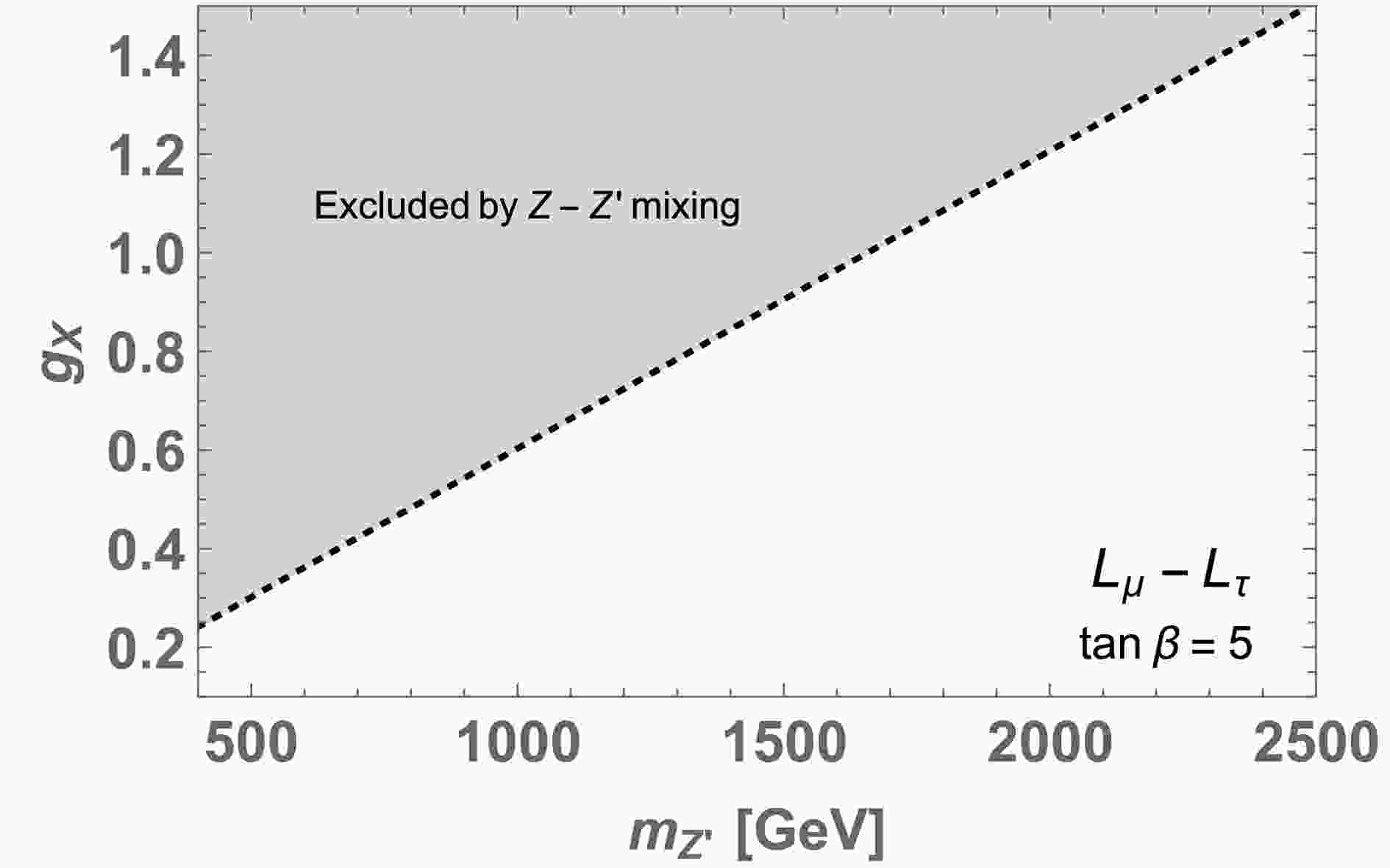
In Fig. 1, we show the region excluded by the EWPT for $ U(1)_{L_\mu - L_\tau} $ with $ \tan \beta =5 $. We observe that $ \mathcal{O}(1) $ gauge coupling is allowed if Z′ mass satisfies 1700 GeV $ \lesssim m_{Z'} $, where the allowed region is also safe from other experimental constraints. We expect a similar Z-Z′ mixing constraint in the other cases, $ U(1)_{L_e-L_\mu} $ and $ U(1)_{L_e-L_\tau} $. This constraint restricts $ v_\varphi \simeq m_{Z'}/g_X $ and can affect the Majorana mass of $ \nu_R $. However, it does not provide much impact in fitting the neutrino mass because we also have Yukawa couplings that are free parameters. In our analysis below, we consider a heavy Z′ and assume Z-Z′ mixing is negligibly small to avoid the EWPT.

Figure 1.  Gray region is excluded by the EWPT for $ U(1)_{L_\mu - L_\tau} $ with $ \tan \beta =5 $.

The mass matrix of the charged lepton is generated via Yukawa interactions in Eq. (1) after electroweak symmetry breaking. Thus, the mass term is given by

where $ \ell(\ell') = \{e, \mu, \tau\} $. Generally, the mass matrix is not diagonal and its structure depends on the model. The possible structures of matrix $ M_e $ are as follows

where $ \times $ indicates a non-zero element. The mass matrix can be diagonalized using bi-unitary matrices $ V_{eL} $ and $ V_{eR} $ transforming $ \ell_L $ and $ \ell_R $; $ M_d^{\rm diagonal} = V_{eL}^\dagger M_e V_{eR} $. Note that such a transformation induces a flavor-changing neutral current (FCNC) for the interaction among Z′ and leptons owing to lepton flavor dependent charges, and it is strongly constrained by LFV search experiments [8]. Here, we illustrate an LFV constraint in a simple case. First, the Z′ interaction for charged leptons is given by

where $ Q_{L_{\alpha -\beta}} $ indicates a diagonal matrix whose elements are $ L_\alpha - L_\beta $ charge, e.g. $ Q_{L_e - L_\mu} = (1,-1,0) $. The FCNC appears when $ V^\dagger_{eL(eR)} Q_{L_\alpha - L_\beta} V_{eL(eR)} $ is not a diagonal matrix. As an example, we consider $ M_e $ of model (3) in Eq. (19) with $ (M_e)_{23} =0 $ for simplicity. Subsequently, focusing on e-μ sector, the mass matrix is expressed by

Selecting $ \delta m \ll M_\mu $, this matrix can be approximately diagonalized by

where $ m_e \sim M_e $ and $ m_\mu \sim M_\mu $. Because model (3) is the $ U(1)_{L_e - L_\tau} $ case, the LFV interaction is approximately given by

Thus, the experimental constraint for $ \mu \to ee \bar e $ process is the most stringent one for the heavy Z′ case ³; it is induced via a virtual Z′ as $ \mu \to e Z'^* \to ee\bar{e} $. We can estimate the decay width and branching ratio (BR) as

where $ G_F $ is the Fermi constant. Applying the current limit $ BR(\mu \to ee \bar e) \lesssim 10^{-12} $ , we obtain

Thus, $ \delta m/m_\mu $ should be very small as $ \delta m/m_\mu \lesssim \mathcal{O}(10^{-5}) $ when $ g_X = \mathcal{O}(1) $, and $ m_{Z'} $ is the TeV scale. Note that we will obtain looser constraints when we consider the LFV decay of an τ lepton. In the numerical analysis below, we assume that off-diagonal elements of the matrix is negligibly small and $ V_{eL(eR)} \simeq 1 $ for simplicity.

After spontaneous symmetry breaking, we obtain the Dirac mass $ M_D $ between $ \nu_L $ and $ \nu_R $ ($ \overline{\nu_L} M_D \nu_R $) and the Majorana mass $ M_R $ of $ \nu_R $. These mass matrices are given by

The structure of these matrices differs for each model. For $ M_D $, we determine the structure as follows:

We also determine the structure of $ M_R $ for each model such that

where the structure is the same when a gauge symmetry of the models is identical.

The neutrino mass in type-I seesaw model is given by

We then express the active neutrino mass matrix as

where κ has a mass dimension, and $ \tilde m_\nu $ is dimensionless. The neutrino mass matrix $ m_\nu $ is diagonalized using a unitary matrix $ V_{\nu} $ via $ D_\nu=|\kappa| \tilde D_\nu= V_{\nu}^T m_\nu V_{\nu}=|\kappa| V_{\nu}^T \tilde m_\nu V_{\nu} $. Thus, $ |\kappa| $ is determined by

where $ \Delta m_{\rm atm}^2 $ is atmospheric neutrino mass-squared splitting, and NO and IO represent the normal and inverted orderings, respectively, of neutrino mass eigenvalues. Subsequently, the solar mass squared splitting can be expressed in terms of $ |\kappa| $ as follows:

which can be compared with the observed value. The observed mixing matrix is defined by $ U=V^\dagger_{eL} V_\nu $ ⁴, where it is parametrized using three mixing angles $ \theta_{ij} (i,j=1,2,3; i < j) $, one CP violating Dirac phase $ \delta_{CP} $, and two Majorana phases $ \alpha_{21},\alpha_{31} $ as follows:

Here, $ c_{ij} $ and $ s_{ij} $ denote $ \cos \theta_{ij} $ and $ \sin \theta_{ij} $ ($ i,j=1-3 $), respectively. Matrix U is identified as the Pontecorvo-Maki-Nakagawa-Sakata (PMNS) matrix [30, 31]. Each of the mixings is given in terms of the component of U as follows:

The Dirac phase $\delta_{\rm CP}$ is given by computing the Jarlskog invariant as follows:

where $\delta_{\rm CP}$ be subtracted from π if $\cos \delta_{\rm CP}$ is negative. The Majorana phases $ \alpha_{21},\ \alpha_{31} $ are determined as

where $\alpha_{21}/2,\ \alpha_{31}/2-\delta_{\rm CP}$ are subtracted from π, when $\cos \left( \dfrac{\alpha_{21}}{2} \right),\ \cos \left(\dfrac{\alpha_{31}}{2} - \delta_{\rm CP} \right)$ are negative. In addition, the effective mass for the neutrinoless double beta decay is given by

where its observed value could be tested in experiments such as KamLAND-Zen [32], LEGEND [33], and nEXO [34].

In this section, we discuss neutrino observables such as masses, mixings, and CP-phases in our models. These values are numerically estimated because structures of the neutrino mass matrix are too complex to obtain analytic solutions for neutrino observables. In the numerical calculation, we modify the neutrino mass matrix as

where $ \tilde{M}_D \equiv M_D/(M_D)_{11} $ and $ \tilde{M}_R= M_R/(M_R)_{kk} $ with $ (M_R)_{kk} $ being a non-zero diagonal element of $ M_R $ in Eq. (30). The scaling factor $ \dfrac{(M_D)_{11}^2 }{(M_R)_{kk}} $ is identified as κ in Eq. (32) that will be evaluated using Eq. (33). Subsequently, we scan the elements of $ \tilde{M}_D $ and $ \tilde{M}_R $ in the range of

where we consider these matrix elements do not have large hierarchy. Note that the elements are generally complex, and we remove phases of diagonal elements of matrix $ M_D $ by redefining phases of lepton fields without loss of generality. The neutrino observables are numerically estimated using the formulas in the previous section to explore the tendency in each model. In the analysis, we adopt NuFit 5.2 neutrino data [18] for the values of $ \{\sin \theta_{12}, \sin \theta_{23}, \sin \theta_{13}, \Delta m^2_{\rm atm}, \Delta m^2_{\rm sol}\} $ within the 3σ range as

Subsequently, we search for values of $ (\tilde{M}_{D,R})_{ij} $ reproducing these 3σ ranges of the observables. Here, we focus on the NO case and check if we can obtain the sum of neutrino masses $ \sum m_\nu $ satisfying the constraint of CMB+DESI, $ \sum m_\nu < 70 $ meV. As a result, we find that models (2) and (4) are disfavored to fit the neutrino data within 3σ, whereas the other models have allowed parameter sets to fit the data. Additionally, we do not have a clear correlation between neutrino mixing angles and the other observables owing to increased free parameters compared with minimal scenarios. For the allowed models, we show some observables such as sum of masses and phases as our predictions.

In Fig. 2, we show $ \langle m_{ee} \rangle $ and $ m_1 $ (the lightest neutrino mass) for the allowed parameter points in each model. The horizontal lines shows the current constraint from KamLand-Zen [32] and the future prospect in nEXO [34] with energy-density functional (EDF) theory for the nuclear matrix element. The distributions are almost similar in these models and some points can be tested in future neutrinoless double beta decay experiments.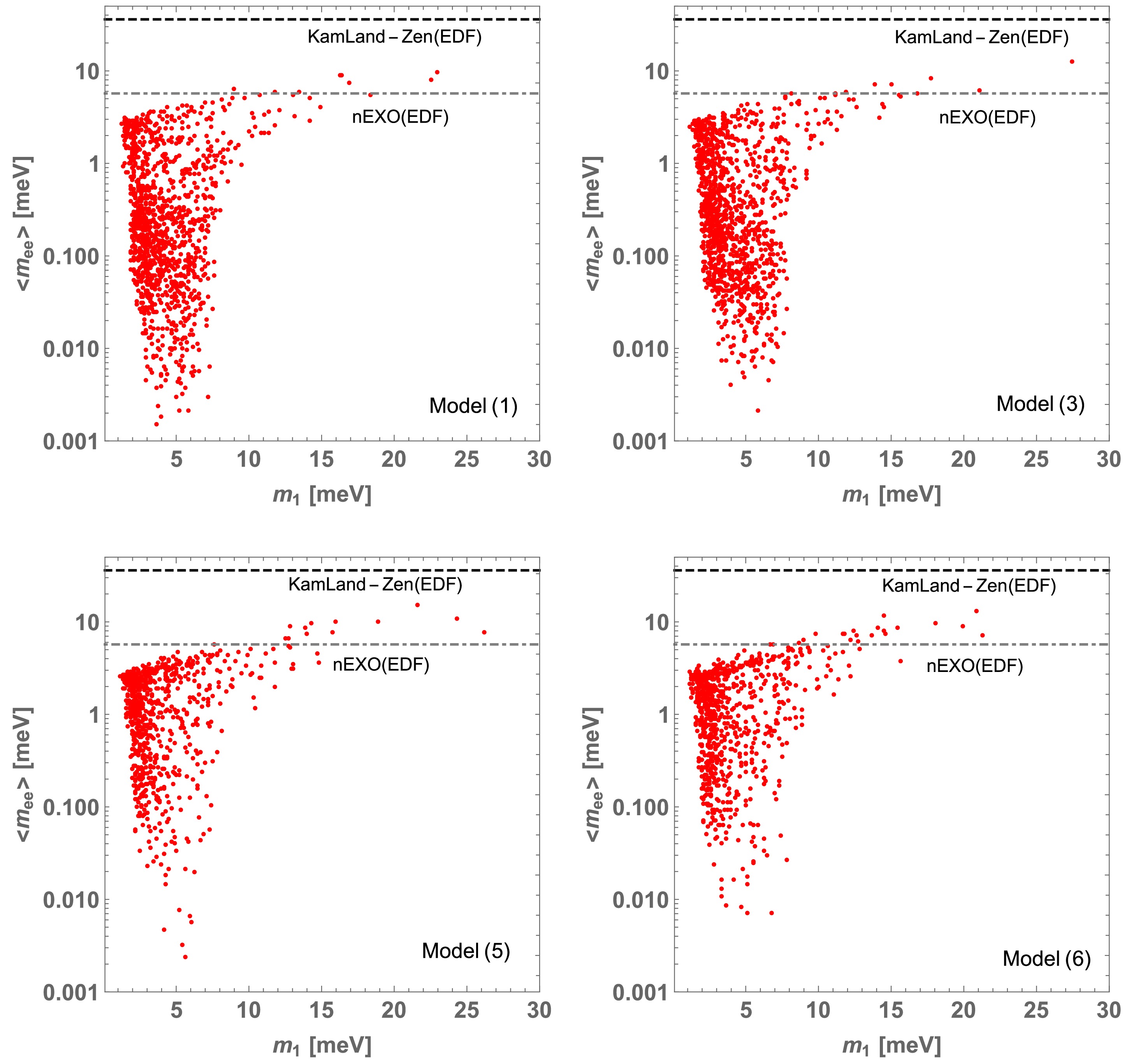

Figure 2.  (color online) Predicted values on the $ \{m_1, \langle m_{ee} \rangle \} $ plane for allowed parameter points in each model.

In Fig. 3, we show $ \sum m_\nu $ and $ \delta_{\rm CP} $ for the allowed parameter points in each model. The vertical line indicates the upper limit using CMB+DESI data. We find a correlation between $ \sum m_\nu $ and $ \delta_{\rm CP} $ where models (1) and (6) [(3) and (5)] exhibit similar behavior. They exhibit ditinguishable behavior in which one tends to provide a small $ \sum m_\nu $ at $ \delta_{\rm CP} \sim 200^{\circ} $, and the other one tends to provide a small $ \sum m_\nu $ at $ \delta_{\rm CP} \sim 0^{\circ}(360^{\circ}) $. We also indicate the 1(3)σ range of the $ \delta_{\rm CP} $ value in the light-blue (cyan) region. These two types of distributions can be distinguished if we have more precision for $ \sum m_\nu $ and $ \delta_{\rm CP} $ in the future.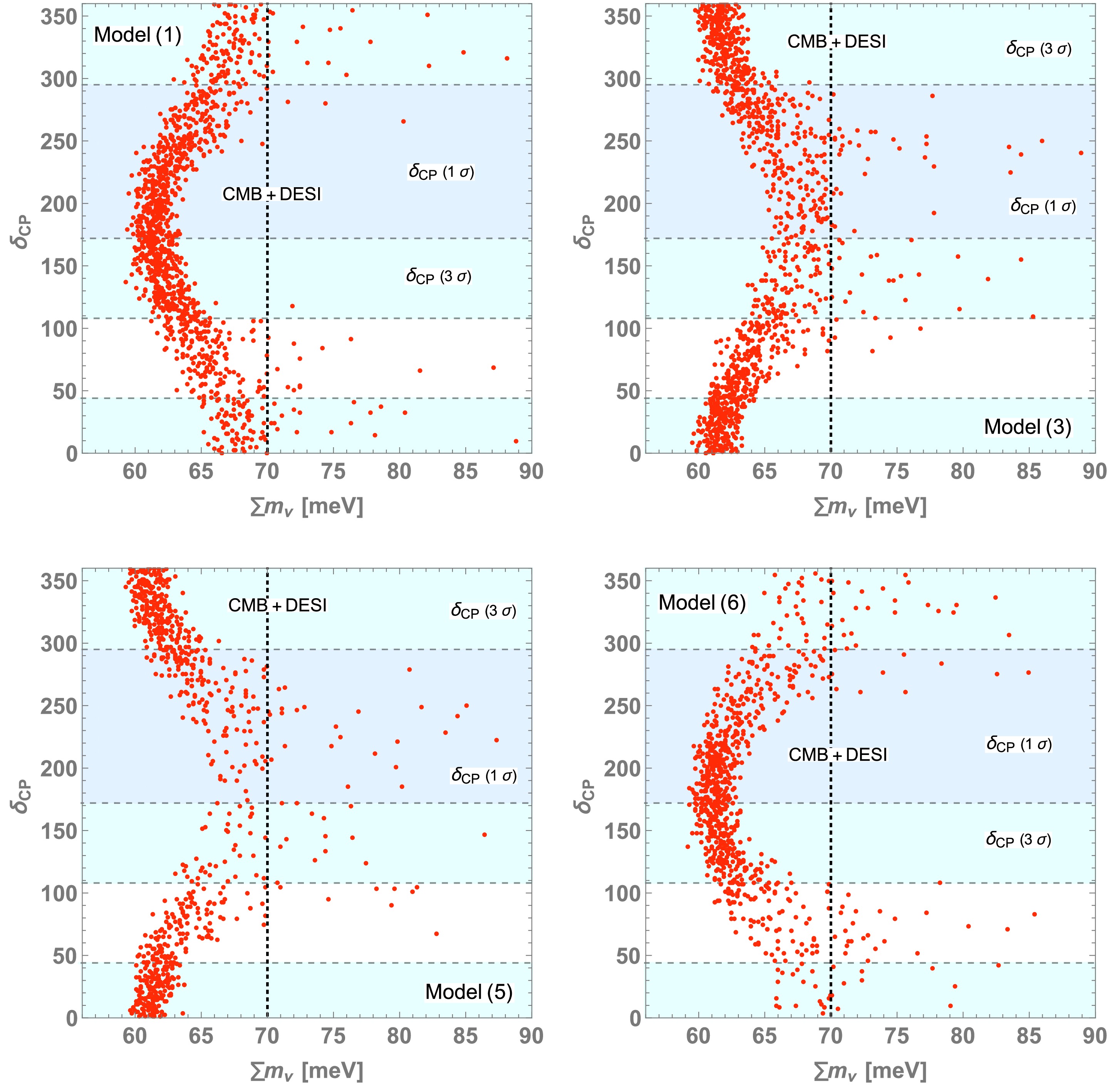

Figure 3.  (color online) Predicted values on the $ \{\sum m_\nu, \delta_{\rm CP} \} $ plane for allowed parameter points in each model. The light-blue (cyan) region indicates 1(3)σ range of $ \delta_{\rm CP} $ value.

Figures 4 and 5 show $ \delta_{\rm CP} $-$ \alpha_{21} $ and $ \delta_{\rm CP} $-$ \alpha_{31} $ values for the allowed parameter points in each model. We find some correlations among phases, where the correlations of $ \delta_{\rm CP} $-$ \alpha_{21} $ in models (1) and (6) [(3) and (5)] exhibit similar behavior. In each case, the value of $ \alpha_{21} $ is concentrated around 100−250 degrees. In contrast, the correlations of $ \delta_{\rm CP} $-$ \alpha_{31} $ are different in each model. In these plots, we show the 1(3)σ range of $ \delta_{\rm CP} $ in the light-blue region similar to Fig. 3. In addition, we also show the correlation between $ \alpha_{21} $ and $ \alpha_{31} $ in Fig. 6, where models (1) and (6) [(3) and (5)] exhibit a similar behavior.

Figure 4.  (color online) Predicted values on the $ \{\delta_{\rm CP}, \alpha_{21} \} $ plane for allowed parameter points in each model. The light-blue (cyan) region also indicates 1(3)σ range of the $ \delta_{\rm CP} $ value.

Figure 5.  (color online) Predicted values on the $ \{\delta_{\rm CP}, \alpha_{31} \} $ plane for allowed parameter points in each model. The light-blue (cyan) region is the same as in Fig. 4.

Figure 6.  (color online) Predicted values on the $ \{\alpha_{21}, \alpha_{31} \} $ plane for allowed parameter points in each model.

We have discussed neutrino observables in $ U(1)_{L_\alpha - L_\beta} $ models, for which we introduce two Higgs doublet and one singlet scalar fields with non-zero charges under new $ U(1) $ as extensions of minimal models that have only one new scalar field. The six models are characterized by the choice of $ U(1)_{L_\alpha - L_\beta} $ gauge symmetry and its charge assignment to the two Higgs doublet. We have then formulated a scalar sector, neutral gauge bosons, a charged lepton mass matrix, and a neutrino mass matrix in the models. The structure of neutrino mass matrix is still restricted by the gauge symmetry but the number of free parameters is increased compared with minimal cases.

In this work, we have focused on the neutrino sector and numerically analyzed neutrino observables. Subsequently, we have determined four models can fit the current neutrino data in 3σ and satisfy constraints on the sum of neutrino mass including recent DESI and Planck data for normal ordering that excludes minimal models under the ΛCDM cosmological model. Although we do not have a correlation between the neutrino mixing angle and other observable because of increased free parameters, we have found some correlations between some observables such as the sum of the neutrino mass and CP phases. In particular, we have found two types of distinguishable distributions on the $ \{\sum m_\nu, \delta_{\rm CP} \} $ plane that can be tested in the future to increase the precision for these observables. Some correlations are also observed among CP phases, although measuring them directly is difficult. To further distinguish the models, we would require to explore Higgs and Z′ physics, for example, searching for collider signals that are specific in the models. The analysis of these physics is beyond the scope of this paper and it is left for future works.