Effects of nuclear deformation and surface polarization on proton-emission half-lives

Proton radioactivity is a process in which one proton is spontaneously emitted from the parent nucleus. This rare decay phenomenon was first observed in $ ^{53}\text{Co}^m $ in 1970 [1]. Subsequently, ground-state proton emissions were reported for $ ^{151}\text{Lu} $ [2] and $ ^{147}\text{Tm} $ [3]. To date, over 40 proton emitters, ranging from $ ^{53}\text{Co}^m $ to $ ^{185}\text{Bi} $, have been experimentally identified, including both ground-state and isomeric transitions. These proton emitters, characterized by their negative proton separation energy, are usually the neutron-deficient nuclei close to the proton drip line, which represents the fundamental limit of nuclear existence [4]. Thus, research studies on proton radioactivity would provide valuable insights into the nuclear structures of proton-rich nuclei and the properties of exotic nuclei beyond the stability limit.

To investigate the mechanism of proton emission, various theoretical models, such as the Gamow-like model [5], coupled channels description [6, 7], unified fission model (UFM) [8, 9], effective liquid-drop model (ELDM) [10], generalized models [11, 12] liquid-drop model (GLDM), and covariant density functional theory (CDFT) [13, 14], have been developed. Among these theoretical models, the key point in studying proton emission is determining daughter-proton interactions, for which well established approaches include the use of the Woods-Saxon potential [15], $ \cosh $ potential [16], Jeukenne, Lejeune, and Mahaux (JLM) interaction [17], density-dependent M3Y interaction (DDM3Y) [17−19], Skyrme interaction [20, 21], and Yukawa effective interaction [22], among others. Within the well constructed interactions, the penetration probability could then be determined using the Wentzel–Kramers–Brillouin (WKB) approximation [17, 18, 23], distorted wave Born approximation (DWBA) [15], and other methods. All of these theoretical methods could give satisfactory descriptions of proton emission from different perspectives.

However, nuclear surface polarization, an exotic phenomenon linked to the geometry of nuclei and the anisotropic diffuseness of nuclear density distribution, has not been included in previous research studies on proton emission. In Ref. [24], researchers successfully developed a parametrization of surface polarization for deformed nuclei, calculating the corresponding parameters of various nuclides using energy density functional (EDF) theory based on the Skyrme effective interaction. In Refs. [25−27], the authors proposed an improved density dependent cluster model, with which they incorporated the anisotropic nuclear surface diffuseness of the deformed nucleus into the study of α-decay and cluster radioactivity, as well as explored the effects of nuclear diffuseness anisotropy and polarization on their half-lives. Within this correction, the improved model known as DDCM+ significantly enhanced its accuracy compared with that of the original model. Inspired by these works [25−27], we are now, in this work, focusing on investigating the effect of polarization on proton radioactivity.

Recently, two branches of proton emission from the high angular momentum excited state $ 19/2^- $ of $ ^{53}\text{Co}^m $ have been successfully identified in an experiment [28]. As the first observed proton emitter, $ ^{53}\text{Co}^m $ is a subject of research that is crucial for understanding high spin neutron-deficient nuclei, whereas its daughter nucleus, $ ^{52}\text{Fe} $, holds significant value in astrophysics research as the endpoint of the $ rp $-process at specific temperature and density conditions [29−31]. Additionally, it provides an opportunity to study the exchange symmetry between neutrons and protons in the $ fp $-shell [32]. In this work, the newly observed proton emission branches are also included, which is expected to deepen our understanding of $ ^{53}\text{Co}^m $.

The remaining parts of this article are organized as follows. The details of the theoretical framework are presented in Sec. II. In Sec. III, we first discuss the effects of deformation and polarization on the proton decay width and spectroscopic factors. Then, we continue with presenting the theoretical half-lives, for which a new deformation and diffuseness dependent spectroscopic factor form is proposed. Notably, the newly observed proton-emission branches of $ ^{53}\text{Co}^m $ are also discussed. Finally, a summary is given in Sec. IV.

Most proton emitters are far from magic nuclei, so the deformation of daughter nuclei is usually not negligible. On the other hand, the deformation of a proton is extremely small, so the system is constructed as comprising a proton and a deformed nucleus. The total interaction between the proton and daughter nucleus is

where r is the distance between the centers of the emitted proton and daughter nucleus, and θ is the polar angle with respect to the axis of deformation serving as the polar axis. A proton to be emitted from its parent nucleus is in the quasi-bound state, denoted by $ n\ell_j $, and is emitted by a tunneling phenomenon through the Coulomb potential barrier. The reduced mass of this binary system is $m_\mu=m_pm_D/ (m_p+m_D)$, where $ m_p $ and $ m_D $ are the masses of the proton and daughter nucleus, respectively.

In this work, the nuclear potential $ V_N(r,\theta) $ is chosen to be the Woods-Saxon potential to facilitate the consideration of deformation and polarization:

For a spherical nucleus, the radius parameter $ R_N $ and diffuseness parameter $ a_N $ are both constants. However, for an axially deformed nucleus, the radius of the potential is changed for each θ, which can be expanded by spherical harmonics as follows:

where $ \beta_2 $ and $ \beta_4 $ are the quadrupole and hexadecapole deformation parameters, respectively, and $ Y_{\ell m} $ refers to spherical harmonics. Additionally, nuclear surface polarization makes $ a_N $ lose anisotropy and be a function of θ. Considering the difference between the normal and radial directions of the deformed surface, the final diffuseness parameter with axial deformation and polarization is given by [24]

where $ \tilde{\beta}_2 $ and $ \tilde{\beta}_4 $ are polarization parameters, representing the mode and degree, respectively, of the nuclear surface polarization.

The next part of the interaction potential is the Coulomb potential. Under the assumption that the spherical daughter nucleus has a uniformly distributed charge, the Coulomb potential created by the charge of the nucleus can be easily calculated using classical electrodynamics, based on which it is independent of the orientation angle θ:

where $ Z_De $ and $ Z_pe $ are the charges of the daughter nucleus and a single proton, respectively, and $ R_{C0} $ is the radius of the charge distribution. However, the deformed Coulomb potential cannot be determined by changing the radius straightforwardly. Although deformation of the Coulomb potential is usually considered in a density dependent model, this cannot give an analytical result. In this work, we analyze this deformed Coulomb potential via multipole expansion. In spherical coordinates, the anisotropy Coulomb potential is expanded as [33]

where $ K_\lambda(r,\theta,\phi) $ is a function of Coulomb radius $ R_C(\theta,\phi)=R_{C0}\left[1+\beta_2Y_{20}(\theta)+\beta_4Y_{40}(\theta)\right] $

In our work, the axial deformation is taken into account, and thus, the radius $ R_C $ and $ K_\lambda $ are independent of ϕ, whereas the terms that include ${\rm e}^{{\rm i}n\phi^\prime}$ in $ Y^*_{\lambda\mu}(\theta^\prime,\phi^\prime) $ will be $ 0 $ after integration; as a result, only the $ \mu=0 $ terms survive when $ \lambda\neq0 $. Finally, we derive the final expression of the axially deformed Coulomb potential to be

which is the multipole expansion for the Coulomb potential of an axially deformed nuclei, where λ can take only even numbers for its value. The diffuseness of charge distribution is neglected in this result, which is justified by the limited impact at large distances of the charge diffuseness within a confined area on the Coulomb potential, so the expanded deformed Coulomb potential as defined in Eq. (8) with neglected charge diffuseness is used in this work.

The third component of the potential is the spin-orbit potential. In contrast to an α particle, an emitted proton has spin angular momentum, so the spin-orbit interaction potential should be considered. The state of proton $ j^\pi $ is determined by the selection rule for angular momentum and parity in the proton emission process [34, 35]:

where $ I_{P,D} $ and $ \pi_{P,D} $ are the spins and parities of the parent and daughter nuclei, respectively, and j is the total angular momentum of the emitted proton. The minimum value among all possible j is adopted in our calculations [27], except for some certain proton emitters determined in previous research [4, 11, 36]. Based on the quantum number $ \ell $ and j obtained above, the spin-orbit interaction is expressed in Thomas form [15]:

where $ V_{so0} $, $ R_{so} $ , and $ a_{so} $ are the depth, radius, and diffuseness, respectively. For a more concise presentation, the values of the parameters adopted for the interactions are listed in Table 1. Deformation and nuclear surface polarization, expressed in Eqs. (3) and (4), are also applied in this potential, which is similar to a Woods-Saxon potential.

Parameters	Values	Parameters	Values
$ R_{C0} $	$ 1.21A_D^{1/3} $	$ V_{so0} $	$ 6.2 $
$ R_{N0} $	$ 1.27A_D^{1/3}-0.1 $ [37, 38]	$ a_{N0} $	$ 0.75 $ [37, 38]
$ R_{so0} $	$ 1.01A_D^{1/3} $	$ a_{so0} $	$ 0.75 $
$ \lambda_\pi^2 $	$ 2.0 $

Table 1.  Parameters of the daughter-proton interaction potential [15, 37, 38]. Values with energy and length dimensions have units of $ \text{MeV} $ and $ \text{fm} $, respectively.

To modify the depth of the nuclear potential, the renormalization factor η is introduced in Eq. (1). In this work, the quasibound state energy is adjusted by η to be equal to the kinetic energy of the emitted proton in experiment, i.e., $ E_0=QA_D/(A_D+1) $, where Q is the decay energy, and $ A_D $ is the number of nucleons in the daughter nuclei. Hence, the approximated depth of the Woods-Saxon nuclear potential is determined for each θ by the quasibound condition [34, 39]

where $ r_{1,2,3}(\theta) $ are three classical turning points at θ, i.e., the roots of $ V(r,\theta)=E_0 $. G is the global quantum number determined by the Wildermuth condition [4], which has been used in a number of research studies on proton radioactivity [4, 9, 11, 39]:

From the viewpoint of the shell model, excluding highly excited proton emitters, G usually takes a value of $ 4 $ or $ 5 $ [4, 11]. The quantum number n denotes the nodes of the radial wave function of the proton, excluding the origin.

To determine the decay width, the WKB approximation, a semiclassical method for its calculation, was employed. However, to improve the accuracy of calculation, in this work we choose to use a quantum method, in which the energy and wave function of the quasibound proton should be calculated. Two-potential approach is a method by which to obtain them [15], but aiming to avoid approximations and decrease possible errors, we choose to directly solve the quasibound wave function. Because the Coulomb potential plays a major role at large distances, the boundary condition of the wave function is a spherical outgoing Coulomb wave function [40]:

where $ F_\ell(kr) $ and $ G_\ell(kr) $ are regular and irregular Coulomb wave functions, respectively, and $ N_\ell $ represents a normalization constant. With this boundary condition, the solution of the time-independent Schrödinger equation gives the quasibound wave function and a more accurate depth of $ \eta V_{N0} $.

Based on the interaction potential and the wave function, the decay width, as a function of θ, can be calculated using the distorted wave Born approximation (DWBA) approach [15]:

with $\delta V_C^\theta(r)=V_C^\theta(r)-Z_pZ_D{\rm e}^2/(4\pi\varepsilon_0r)$. Therefore, the total decay width can be expressed as the average by integration along all orientation angles:

The relationship between the decay width and half-life is $ T_{1/2}=\hbar\ln{2}/(S_p\Gamma) $, where $ S_p $ is the spectroscopic factor. The value of $ S_p $ is closely related to the structure properties of proton emitters. In spherical cases, it can be calculated using relativistic mean field (RMF) models combined with BCS pairing methods [4], accounting for the probability that the orbital of the emitted proton is unoccupied in the assumed spherical daughter nucleus [34, 41, 42]. However, in deformed cases, the deformation would require an important correction to the value of $ S_p $ . To calculate this, the internal component can be multiplied by the amplitude to find more accurately the final proton Nilsson state in the initial quasi-particle state [34].

In this section, we intend to explore the effects of deformation and polarization on half-lives and reproduce the available experimental data on proton emission. The parameters involved in the interaction potential are listed in Table 1, and most of them are taken from Ref. [15]. Recent research studies [41, 42] on the radius and diffuseness of the Woods-Saxon potential yield different values from those in Ref. [15], so we adopt the new values instead, which are determined based on Skyrme energy-density functional approaches. In our calculations, the masses of parent and daughter nuclei are taken from Ref. [43], the spin-parities of parent and daughter nuclei are mainly from Refs. [43, 44], the deformation parameters of daughter nuclei are obtained from Ref. [45], and the kinetic energies $ E_0 $ with uncertainties of emitted protons are taken from experimental decay energies [36]. The experimental half-lives on proton emission, to be used for comparison, are taken from Refs. [43, 44] . The spectroscopic factors $ S_p^{\text{RMF}} $ calculated using RMF are mainly from Ref. [11].

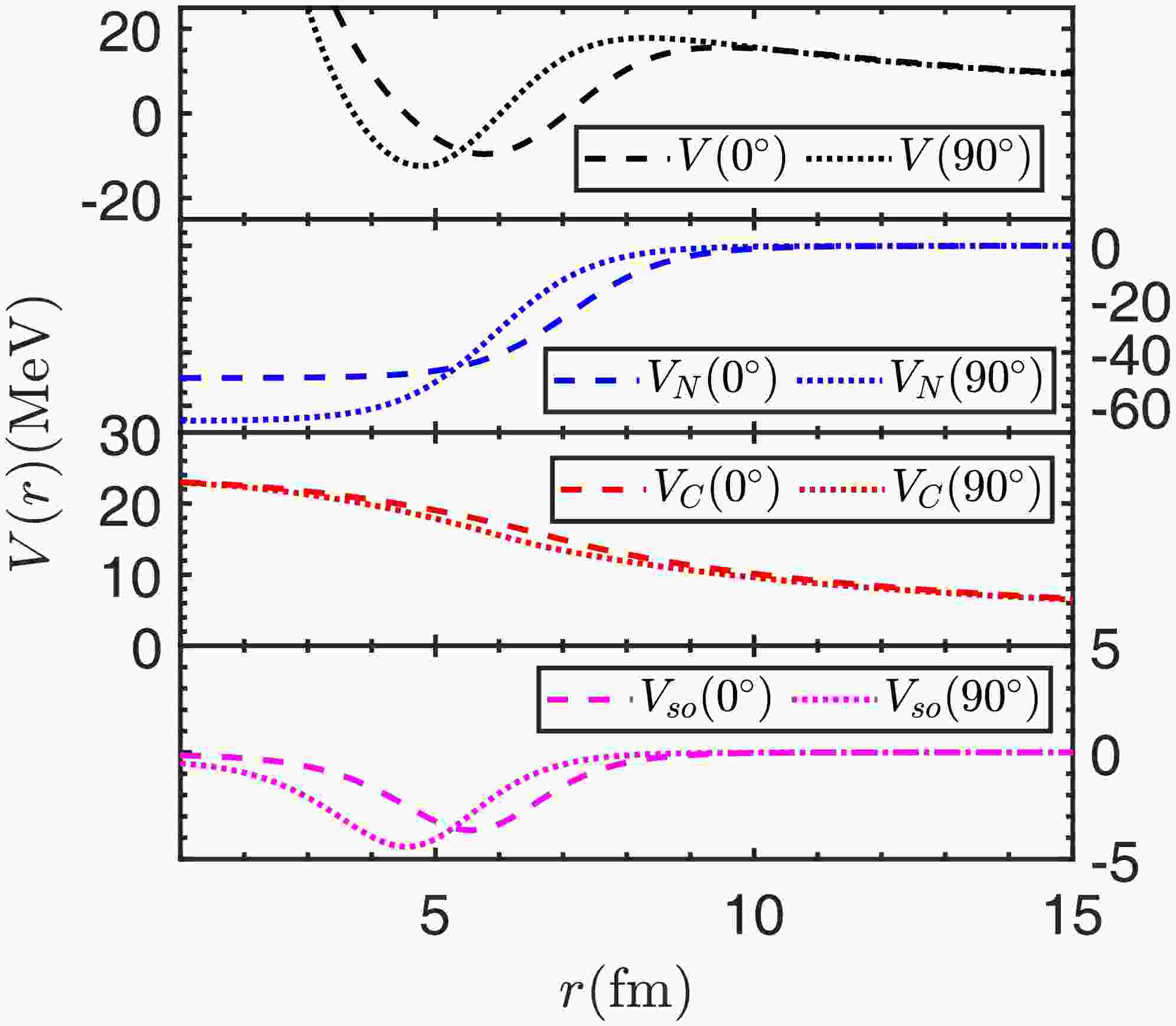
In this subsection, we focus on the deformation of daughter nuclei, which has influence on the daughter-proton interaction and spectroscopic factor. Note that the nuclear surface polarization is not taken into account at this stage. To examine the reliability of our calculation, we selected a highly deformed proton emitter, for instance, $ ^{145}\text{Tm} $ , to allow a more detailed analysis of the deformation effect.

Figure 1 illustrates the total potential $ V_N(r,\theta) $ for the proton emitter $ ^{145}\text{Tm} $ in two directions, $ \theta=0^\circ $ and $ \theta=90^\circ $, together with the three components: the Woods-Saxon nuclear potential $ V_N(r,\theta) $, Coulomb potential $ V_C(r,\theta) $, and spin-orbit interaction potential $ V_{so}(r,\theta) $. The centrifugal potential is not shown in the figure because it has no dependence on the direction θ. As for the total potential, it is evident that the proton to be emitted is bound on a quasibound state by the potential barrier. Although the main contribution to the barrier comes from the Coulomb potential $ V_C(r,\theta) $, the barrier variation with direction results from the nuclear plus spin-orbit interaction potentials. As one can see, the barrier shape for $ r=6-10 $ fm is a direct outcome of the nuclear plus spin-orbit interaction potentials. The barrier height at $ \theta=90^\circ $ is larger than that at $ \theta=0^\circ $ owing to the positive quadrupole deformation $ \beta_2 $. This would bring in more intense quantum tunneling at $ \theta=0^\circ $ compared with that at $ \theta=90^\circ $. We calculated the decay widths at a discretized grid of direction θ using the DWBA method. Figure 2 shows the decay width of $ ^{145}\text{Tm} $ as a function of direction θ. In view of the symmetry associated with quadrupole and hexadecapole deformations, the angular distribution is shown only for the angles ranging from $ 0^\circ $ to $ 90^\circ $. As one would expect, the decay width at $ \theta=0^\circ $ is much larger than that at $ \theta=90^\circ $, showing an active response to the total potential shown in Fig. 1. The results calculated with and without deformation are also shown for comparison. It is found that the $ ^{144} $Er deformation overall decreases the half-life of the proton emitter $ ^{145}\text{Tm} $.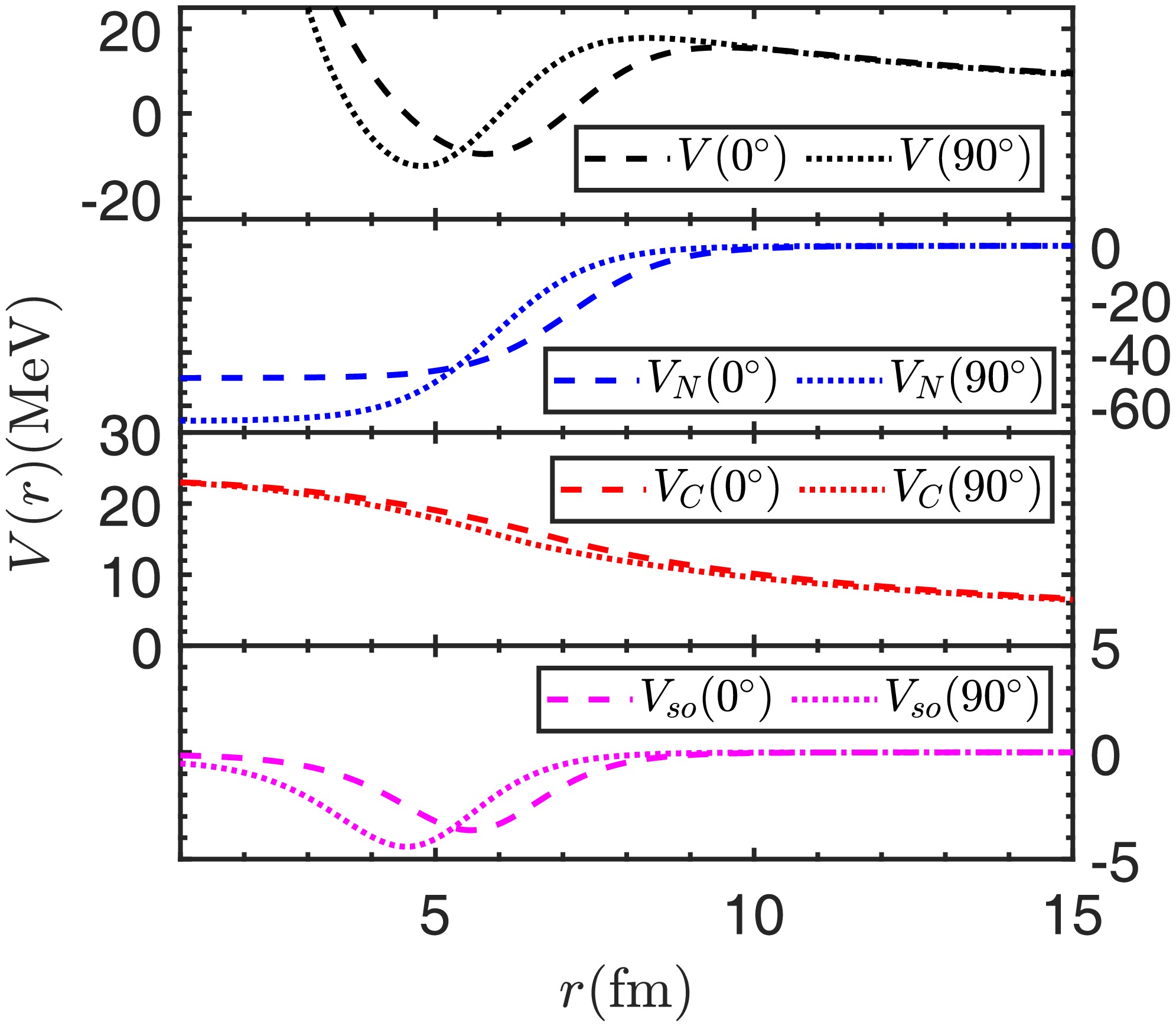

Figure 1.  (color online) Daughter-proton interactions for proton emission of $ ^{145}\text{Tm} $. Total potential and three components, i.e., nuclear potential $ V_N $, Coulomb potential $ V_C $, and spin-orbit potential $ V_{so} $ , are shown in two directions: $ \theta=0^\circ $ (dashed lines) and $ \theta=90^\circ $ (dotted lines).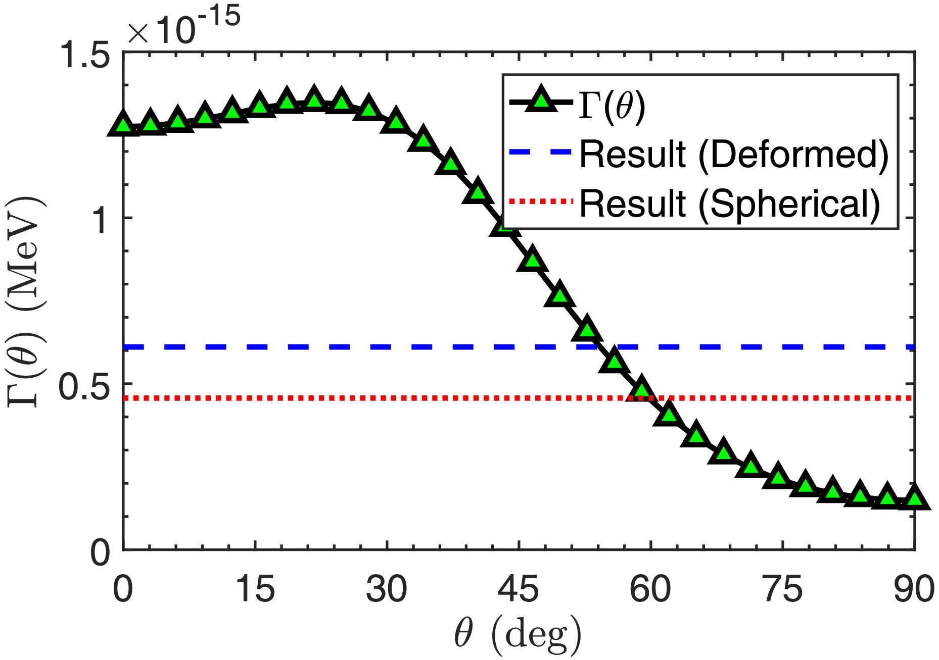

Figure 2.  (color online) Decay width as a function of direction θ for proton emission from $ ^{145}\text{Tm} $ into $ ^{144}\text{Er} $. Black curve with green triangles represents $ \Gamma(\theta) $. Red line corresponds to calculated decay width without deformation. Blue line represents overall decay width calculated using Eq. (15).

Deformation also affects the spectroscopic factor. Recent research studies [16, 36] have detected the logarithmic relationship between $ \log_{10}S_p $ and $ \beta_2 $. In this work, we would like to propose an analytic formula to calculate the spectroscopic factor $ S_p^{\text{def,fit}} $ of various proton emitters. The experimental spectroscopic factors are defined by $ S_p^{\text{exp}}=\hbar\ln2/(T_{1/2}^{\text{exp}}\Gamma) $, where Γ is the decay width calculated using the DWBA method. Figure 3 shows the experimental spectroscopic factors as a function of the quadrupole deformation of daughter nuclei for $ 43 $ proton emitters with the uncertainty of experimental decay energy. For most emitters, excluding $ ^{105} $Sb, the consequent uncertainties of $ S_p $ are not considerable. Therefore, a strong correlation between $ S_p^{\text{exp}} $ and $ \beta_{2} $ is evident: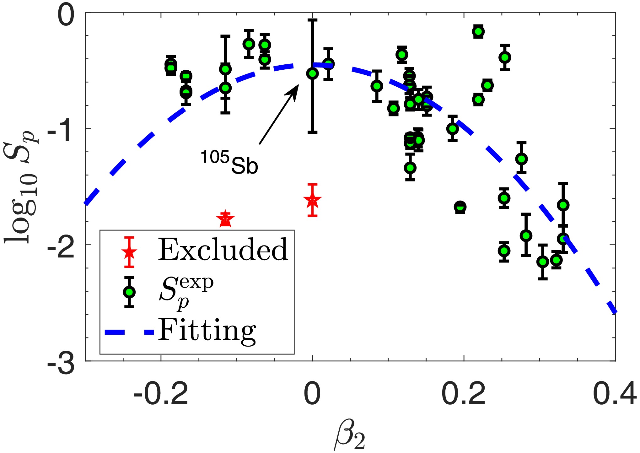

Figure 3.  (color online) Experimental spectroscopic factors $ S_p^{\text{exp}} $ as a function of the quadrupole deformation of daughter nuclei for $ 43 $ proton emitters along with uncertainties arising from experimental decay energies. Excluding $ ^{105}\text{Sb} $, most emitters have small uncertainties. $ ^{185}\text{Bi} $ and $ ^{177}\text{Tl}^m $ are labeled with red pentagrams because of their strong shell effect. Blue lines show the fitting to the experimental spectroscopic factors $ S_p^{\text{def,fit}} $ , excluding those for $ ^{185}\text{Bi} $ and $ ^{177}\text{Tl}^m $.

After fitting to the experimental spectroscopic factors, the parameters in Eq. (16) are determined to be $ b_1=-13.352 $ and $ b_2=-0.452 $. Note that some nuclei near the proton magic number, such as $ ^{185}\text{Bi} $ and $ ^{177}\text{Tl}^m $, are excluded because their strong shell effect dominates the deformation effect. The results for the half-lives related to $ S_p^{\text{def,fit}} $ will be discussed in subsequent subsections.

To summarize this subsection, the deformation of daughter nuclei affects mainly the Woods-Saxon nuclear potential plus spin-orbit coupling potential, resulting in anisotropy in the probability of proton emission along the different directions from proton emitters. On the whole, it has influence on the half-life of proton emission. Meanwhile, an analytic approximate relationship between spectroscopic factors and deformation is explored in detail.

Next, we focus on the proton emitters with polarized daughter nuclei and discuss the effect of nuclear surface polarization. Polarization is parameterized in Ref. [24], where the polarization parameters are given using two functionals SkM* and Sly4 for the nuclei ranging from $ ^{16}\text{O} $ to $ ^{276}\text{Hs} $. Considering that the parameters of the two functionals are similar, we use only the result of the SkM* functional to give an instance with which to analyze the polarization effect. To distinguish the polarization effect from the deformation effect, we first choose three proton emitters, for example, $ ^{105}\text{Sb} $, $ ^{146}\text{Tm} $ , and $ ^{147}\text{Tm} $, with different deformation modes. Here, we changed the polarization parameter $ \tilde{\beta}_2 $ from negative to positive within a certain interval and neglected the effect of $ \tilde{\beta}_4 $. The calculated decay widths are illustrated in Fig. 4. As can be seen, the three cases with different deformations exhibit different behaviors with respect to changes in the polarization parameter $ \tilde{\beta}_2 $. More specifically, the case with positive quadrupole deformation $ \beta_2>0 $ decreases the half-life of $ ^{146} $Tm with increasing polarization parameter $ \tilde{\beta}_2 $, while the case with negative deformation parameter $ \beta_2<0 $ shows the opposite trend with increasing $ \tilde{\beta}_2 $. The case with $ \beta_2=0 $ shows a relatively smooth variation, where both positive and negative quadrupole polarization lead to a small reduction in the half-life of $ ^{105} $Sb. It is obvious that the polarization effect is closely correlated with nuclear deformation.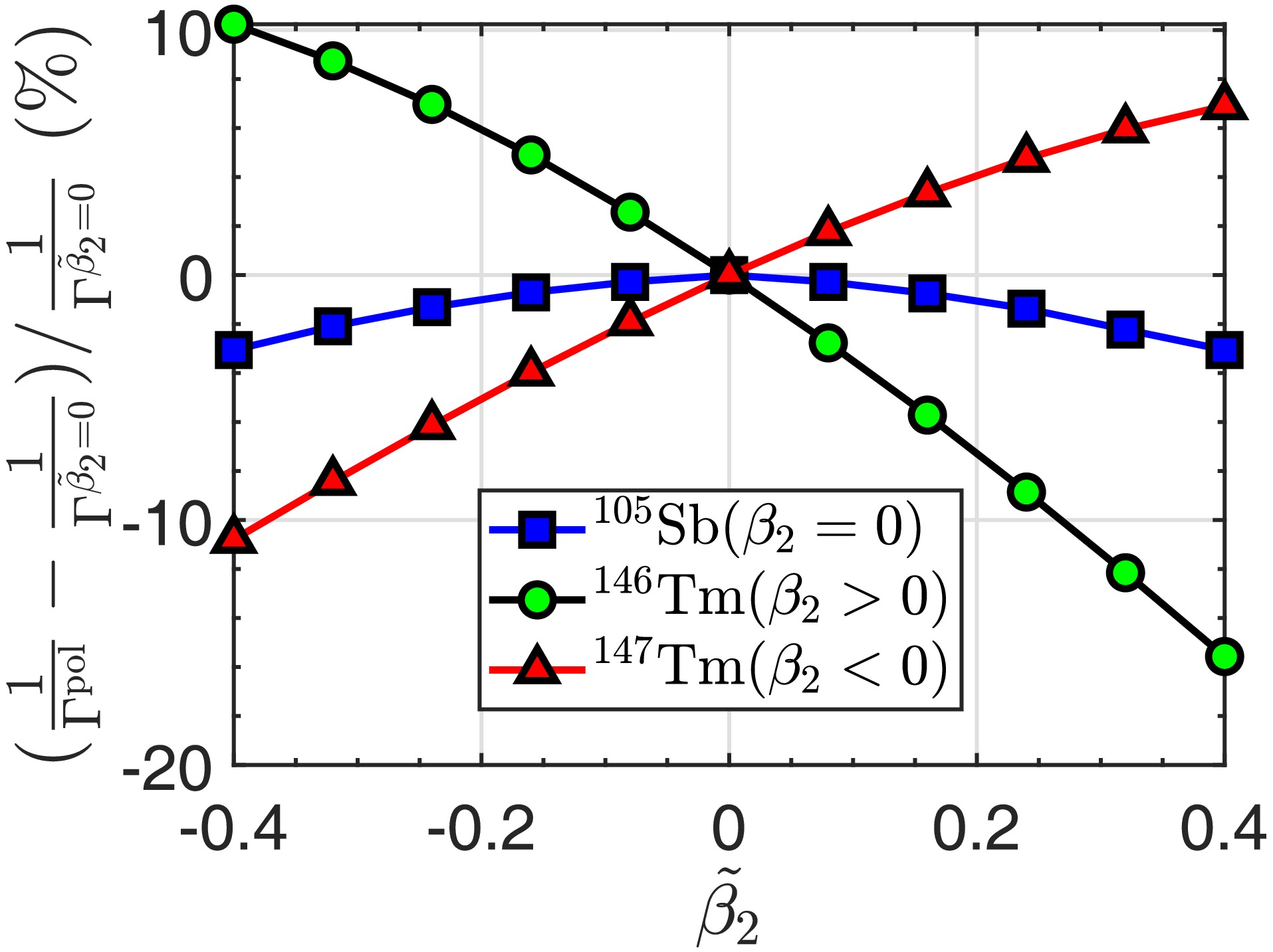

Figure 4.  (color online) Variations in the inverse of calculated decay width $ 1/\Gamma $ as a function of polarization parameter $ \tilde{\beta}_2 $ for three different deformed nuclei: (a) $ ^{146}\text{Tm} $ with prolate deformation ($ \beta_2>0 $), (b) $ ^{105}\text{Sb} $ without deformation ($ \beta_2=0 $), and (c) $ ^{147}\text{Tm} $ with oblate deformation ($ \beta_2<0 $).

To gain a deeper insight into the surface polarization, we also consider the polarization parameters in reality, as obtained from Ref. [24]. Two proton emitters, $ ^{131}\text{Eu} $ and $ ^{171}\text{Au} $ , are chosen for the strong deformation and different polarization modes of their daughter nuclei. For both emitters, the barrier height $ V_p(\theta) $ along each orientation angle is displayed in Fig. 5. The decay widths for each orientation angle are also calculated and shown in the figure. They are compared with the results calculated without polarization $ \tilde{\beta}_{2,4}=0 $. First of all, nuclear surface polarization has influence on the daughter-proton interaction potential and, hence, the decay half-life. Second, different polarizations lead to various changes in the potential and decay width. It can be seen that the polarization effect is more considerable for $ ^{131} $Eu, particularly for small orientation angles θ. In terms of the tendency shown in Fig. 4, the half-life of $ ^{131} $Eu should be enhanced by the polarization effect owing to its prolate daughter nucleus and a negative polarization parameter $ \tilde{\beta}_2 $. However, in actuality, its half-life is still decreased after including the polarization effect. Such an unexpected discrepancy is attributed to the large polarization parameter $ \tilde{\beta}_4>\tilde{\beta}_2 $ in its daughter nucleus $ ^{130}\text{Sm} $. For the proton emitter $ ^{171}\text{Au} $ with the prolate daughter nucleus, a positive $ \tilde{\beta}_2 $ and small $ \tilde{\beta}_4 $ bring in a reduction in its half-life. This is quite consistent with the tendency depicted in Fig. 4.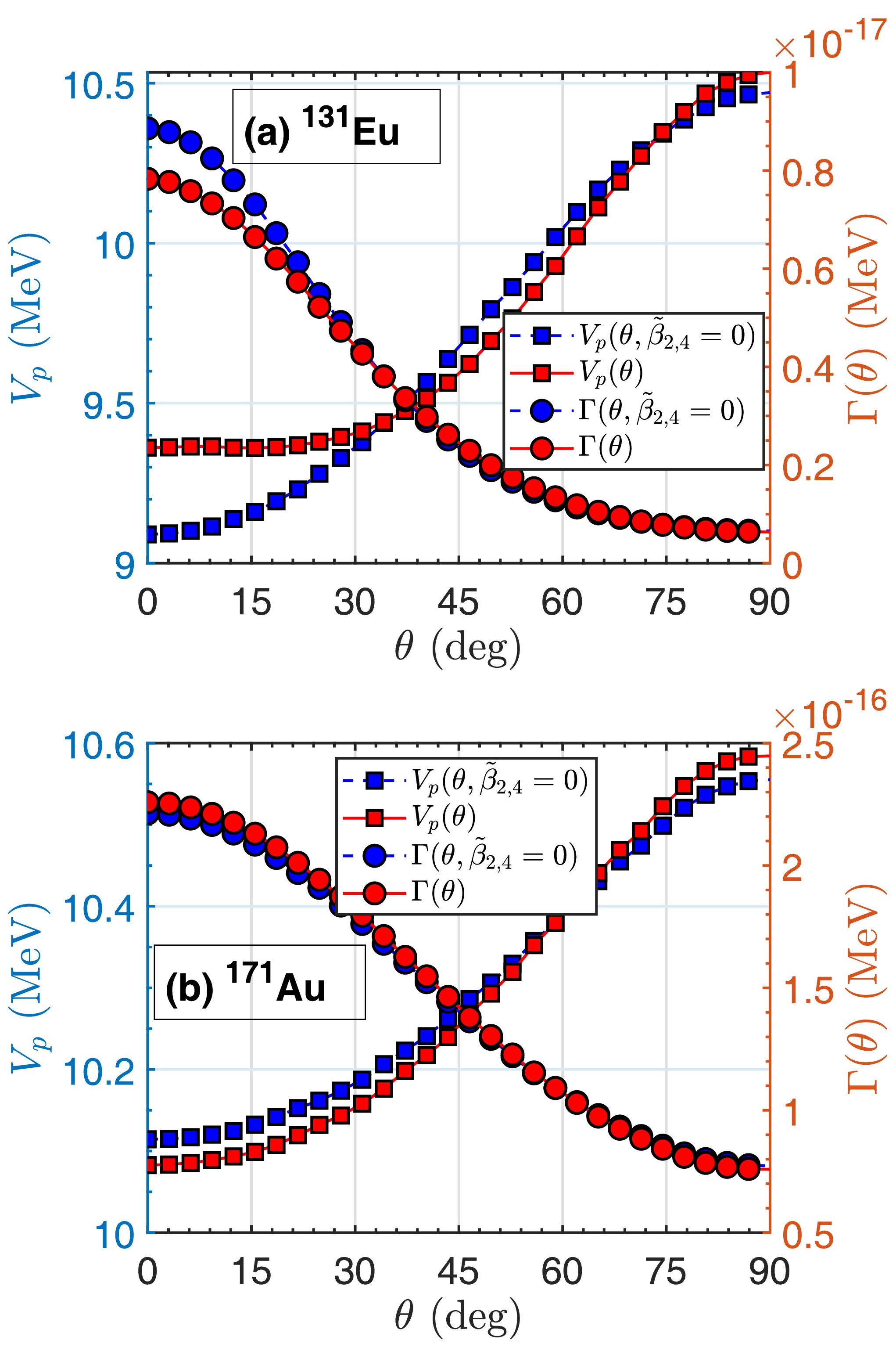

Figure 5.  (color online) Potential barrier height $ V_p(\theta) $ (circles) and decay width $ \Gamma(\theta) $ (squares) as functions of θ in two proton emitters within polarization: (a) $ ^{131}\text{Eu} $ and (b) $ ^{171}\text{Au} $, which have opposite signs for the quadrupole polarization parameters. Blue lines are calculated on the condition of $ \tilde{\beta}_{2,4}=0 $ , for comparison.

In addition to nuclear deformation, nuclear surface polarization also affects the spectroscopic factor $ S_p $. In this work, we propose an average quantity to describe the intensity of polarization:

The experimental spectroscopic factors for all proton emitters with even-even daughter nuclei are shown in Fig. 6. It should be noted that, in this subsection, Γ and $ S_p^{\text{exp}}=\hbar\ln2/(T_{1/2}^{\text{exp}}\Gamma) $ are recalculated with the nuclear surface polarization taken into account. One can see that there is an obvious relationship between $ S_p $ and $ \overline{a}_N $ , except for those special proton emitters with the strong shell effect. For a given $ \beta_2 $, a proton emitter with larger $ \overline{a}_N $ generally exhibits a smaller $ S_p $. The underlying physics of this negative correlation requires further research in the future. Meanwhile, the experimental spectroscopic factors are also shown in Fig. 6 versus the quadrupole deformation $ \beta_{2} $. The correlation between $ S_p $ and $ \beta_{2} $ remains, as illustrated in Fig. 3. Combining the effects of deformation and polarization, we propose a quadratic form for the spectroscopic factor based on the distribution of $ S_p $ in Figs. 3 and 6: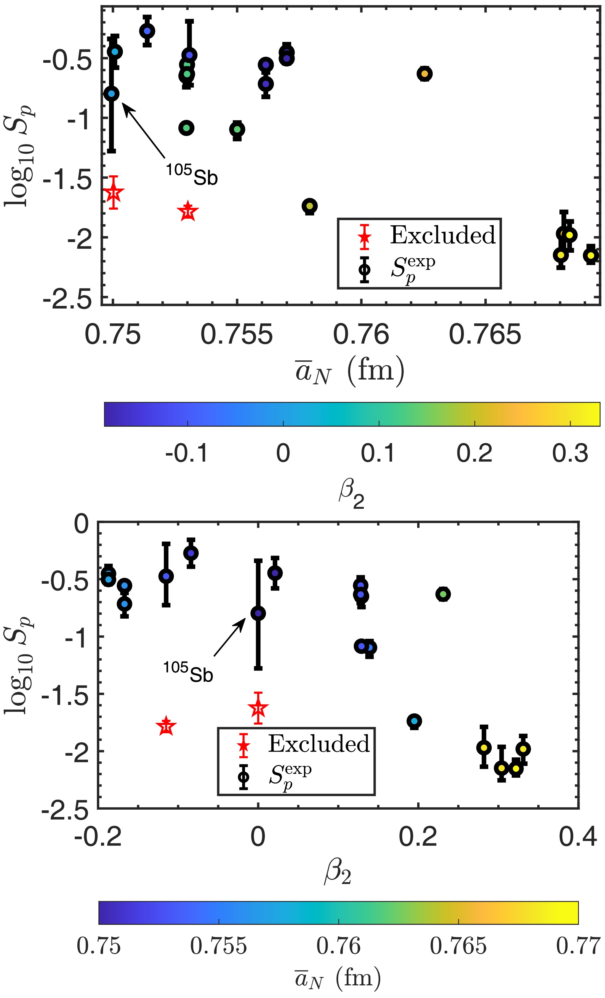

Figure 6.  (color online) Relationship between quadrupole deformation $ \beta_2 $ and average polarization $ \overline{a}_N $ of daughter nuclei and experimental spectroscopic factors $ S_p^{\text{exp}} $ with uncertainties introduced by experimental decay energies. Excluding the two nuclei with strong shell effect, $ ^{185}\text{Bi} $ and $ ^{177}\text{Tl}^m $ , which have been marked out, larger polarization generally indicates a smaller spectroscopic factor. Uncertainties for some emitters are quite small, making those error bars not apparent.

where the diffuseness parameter $ \overline{a}_N $ is in units of fm, and the parameters are determined to be $ c_1=-9.812 $, $ c_2=-1.901 $, $ c_3=-8.649 $, and $ c_4=6.056 $. The corresponding half-lives will be discussed in the next subsection. Similar to the analysis in the previous subsection, considering the experimental uncertainty of Q, most emitters do not have considerable uncertainties for $ S_p $, so the uncertainties are temporarily neglected in the fitting.

In the subsections above, we discussed the effects of deformation and polarization on decay width and spectroscopic factor, so now we can discuss the half-lives $ T_{1/2}=\hbar\ln{2}/(S_p\Gamma) $ of various proton emitters. First, based on our theoretical model, we calculated the half-lives of $ 43 $ proton emitters, which have been measured by experiments over the past many decades, via the DWBA method with deformation taken into account. Table 2 shows the results for when deformation is taken into account without polarization. From the nuclear parameters in the table, we use the spectroscopic factors $ S_p^{\text{RMF}} $ calculated based on the RMF theory [11] to determine, under the assumptions that the daughter nuclei are spherical and deformed, the values of $ \log_{10}T_{1/2}^{\text{sph}} $ and $ \log_{10}T_{1/2}^{\text{def}} $, respectively. For comparison, excluding the theoretical result for $ \beta_2 $, we also utilize the experimental deformation parameters [49, 50] in calculation, which are shown in the table with the superscript ex. However, because of a lack of experiments near the proton drip line, only the $ \beta_2 $ of the daughter nuclei of $ ^{105} $Sb and $ ^{109} $I are available. The results show that differences between the theoretical and experimental $ \beta_2 $ do not have considerable effects on the results. Therefore, to ensure consistency of the data used for the calculations, only theoretical deformation values were employed in the previous fitting process for $ S_p^{\text{def,exp}} $.

Emitter	$ j^\pi $	$E_0/\text{MeV}$	$ \beta_2 $	$ \beta_4 $	$\log_{10}T_{1/2}^{\text{exp} }/\text{s}$	$ S_p^{\text{RMF}} $	$\log_{10}T_{1/2}^{\text{sph} }/\text{s}$	$\log_{10}T_{1/2}^{\text{def} }/\text{s}$	$ S_p^{\text{def,fit}} $	$\log_{10}T_{1/2}^{\text{def,fit} }/\text{s}$
$ ^{105}\text{Sb} $	$ 5/2^+ $	0.478$ _{-0.015}^{+0.015} $[47]	0.000	0.000	2.049 [43, 44]	0.999	1.561$ _{-0.459}^{+0.507} $	1.561$ _{-0.459}^{+0.507} $	0.353	2.012$ _{-0.459}^{+0.507} $
			$ 0.110^{\text{ex}} $					$ 1.558^{+0.473}_{-0.468} $	0.224	$ 2.174^{+0.473}_{-0.468} $
$ ^{109}\text{I} $	$ 3/2^+ $	0.819$ _{-0.005}^{+0.005} $	0.139	0.056	−4.029 [36]	0.726	−4.945$ _{-0.092}^{+0.056} $	−4.966$ _{-0.074}^{+0.082} $	0.195	−4.396$ _{-0.074}^{+0.082} $
			$ 0.153^{\text{ex}} $					−$ 4.965^{+0.553}_{-0.884} $	0.172	−$ 4.341^{+0.553}_{-0.884} $
$ ^{112}\text{Cs} $	$ 3/2^+ $	0.816$ _{-0.007}^{+0.007} $	0.185	0.052	−3.310	0.369	−3.850$ _{-0.108}^{+0.110} $	−3.878$ _{-0.108}^{+0.100} $	0.123	−3.403$ _{-0.108}^{+0.100} $
$ ^{113}\text{Cs} $	$ 3/2^+ $	0.967$ _{-0.003}^{+0.003} $	0.195	0.054	−4.752	0.373	−5.950$ _{-0.036}^{+0.036} $	−5.998$ _{-0.016}^{+0.046} $	0.110	−5.467$ _{-0.016}^{+0.046} $
$ ^{117}\text{La} $	$ 3/2^+ $	0.807$ _{-0.011}^{+0.011} $ [48]	0.282	0.106	−1.602	0.311	−2.923$ _{-0.178}^{+0.182} $	−3.016$ _{-0.185}^{+0.171} $	0.031	−2.010$ _{-0.185}^{+0.171} $
$ ^{121}\text{Pr} $	$ 3/2^+ $	0.893$ _{-0.010}^{+0.010} $ [48]	0.304	0.087	−2.000	0.122	−3.104$ _{-0.145}^{+0.147} $	−3.233$ _{-0.144}^{+0.147} $	0.021	−2.461$ _{-0.144}^{+0.147} $
$ ^{130}\text{Eu} $	$ 3/2^+ $ [36]	1.031$ _{-0.015}^{+0.015} $	0.331	0.018	−3.046	0.816	−4.478$ _{-0.186}^{+0.190} $	−4.616$ _{-0.186}^{+0.175} $	0.012	−2.790$ _{-0.186}^{+0.175} $
$ ^{131}\text{Eu} $	$ 3/2^+ $	0.952$ _{-0.009}^{+0.009} $	0.331	0.018	−1.699	0.029	−1.972$ _{-0.127}^{+0.128} $	−2.111$ _{-0.110}^{+0.117} $	0.012	−1.734$ _{-0.110}^{+0.117} $
$ ^{135}\text{Tb} $	$ 7/2^- $	1.191$ _{-0.007}^{+0.007} $	0.322	−0.037	−3.027	0.028	−3.475$ _{-0.073}^{+0.074} $	−3.606$ _{-0.072}^{+0.067} $	0.015	−3.322$ _{-0.072}^{+0.067} $
$ ^{140}\text{Ho} $	$ 7/2^- $ [36]	1.098$ _{-0.010}^{+0.010} $	0.276	−0.047	−2.222	0.952	−3.363$ _{-0.121}^{+0.123} $	−3.462$ _{-0.140}^{+0.117} $	0.034	−2.015$ _{-0.140}^{+0.117} $
$ ^{141}\text{Ho} $	$ 7/2^- $	1.182$ _{-0.008}^{+0.008} $	0.253	−0.039	−2.387	0.008	−2.268$ _{-0.087}^{+0.088} $	−2.342$ _{-0.070}^{+0.088} $	0.049	−3.133$ _{-0.070}^{+0.088} $
$ ^{144}\text{Tm} $	$ 11/2^- $	1.713$ _{-0.016}^{+0.016} $	0.254	−0.064	−5.569 [36]	0.558 [42]	−5.554$ _{-0.105}^{+0.106} $	−5.703$ _{-0.104}^{+0.106} $	0.049	−4.644$ _{-0.104}^{+0.106} $
$ ^{145}\text{Tm} $	$ 11/2^- $	1.741$ _{-0.007}^{+0.007} $	0.231	−0.068	−5.499	0.580	−5.764$ _{-0.045}^{+0.045} $	−5.890$ _{-0.045}^{+0.045} $	0.069	−4.962$ _{-0.045}^{+0.045} $
$ ^{146}\text{Tm} $	$ 11/2^- $	1.202$ _{-0.004}^{+0.004} $	0.219	−0.057	−0.810 [43]	0.962	−1.427$ _{-0.044}^{+0.045} $	−1.543$ _{-0.044}^{+0.045} $	0.081	−0.468$ _{-0.044}^{+0.045} $
$ ^{147}\text{Tm} $	$ 11/2^- $	1.066$ _{-0.005}^{+0.005} $	−0.187	−0.022	0.587	0.581	0.448$ _{-0.066}^{+0.067} $	0.378$ _{-0.066}^{+0.067} $	0.121	1.060$ _{-0.066}^{+0.067} $
$ ^{150}\text{Lu} $	$ 11/2^- $	1.274$ _{-0.003}^{+0.003} $	−0.167	−0.035	−1.197	0.497	−1.514$ _{-0.031}^{+0.032} $	−1.571$ _{-0.031}^{+0.031} $	0.150	−1.050$ _{-0.031}^{+0.031} $
$ ^{151}\text{Lu} $	$ 11/2^- $	1.245$ _{-0.003}^{+0.003} $	−0.167	−0.035	−0.896	0.490	−1.077$ _{-0.033}^{+0.033} $	−1.134$ _{-0.033}^{+0.033} $	0.150	−0.620$ _{-0.033}^{+0.033} $
$ ^{155}\text{Ta} $	$ 11/2^- $	1.459$ _{-0.015}^{+0.015} $	0.021	0.000	−2.538	0.422	−2.606$ _{-0.131}^{+0.133} $	−2.607$ _{-0.131}^{+0.133} $	0.349	−2.524$ _{-0.131}^{+0.133} $
$ ^{156}\text{Ta} $	$ 3/2^+ $	1.023$ _{-0.005}^{+0.005} $	−0.063	0.001	−0.842	0.761	−1.122$ _{-0.074}^{+0.074} $	−1.128$ _{-0.065}^{+0.074} $	0.313	−0.742$ _{-0.065}^{+0.074} $
$ ^{157}\text{Ta} $	$ 1/2^+ $	0.941$ _{-0.007}^{+0.007} $	−0.084	0.014	−0.527	0.797	−0.693$ _{-0.117}^{+0.112} $	−0.701$ _{-0.117}^{+0.118} $	0.284	−0.254$ _{-0.117}^{+0.118} $
$ ^{160}\text{Re} $	$ 3/2^+ $ [4]	1.277$ _{-0.005}^{+0.005} $	0.107	0.004	−3.045	0.507	−3.558$ _{-0.054}^{+0.055} $	−3.576$ _{-0.054}^{+0.055} $	0.249	−3.266$ _{-0.054}^{+0.055} $
$ ^{161}\text{Re} $	$ 1/2^+ $	1.206$ _{-0.006}^{+0.006} $	0.128	0.018	−3.357	0.892	−3.833$ _{-0.071}^{+0.071} $	−3.854$ _{-0.063}^{+0.071} $	0.214	−3.233$ _{-0.063}^{+0.071} $
$ ^{166}\text{Ir} $	$ 3/2^+ $	1.161$ _{-0.007}^{+0.007} $	0.140	−0.005	−0.824	0.415	−1.511$ _{-0.090}^{+0.091} $	−1.543$ _{-0.090}^{+0.091} $	0.193	−1.211$ _{-0.090}^{+0.091} $
$ ^{167}\text{Ir} $	$ 1/2^+ $	1.089$ _{-0.006}^{+0.006} $	0.151	−0.004	−1.028	0.912	−1.706$ _{-0.085}^{+0.085} $	−1.717$ _{-0.085}^{+0.085} $	0.175	−1.001$ _{-0.085}^{+0.085} $
$ ^{170}\text{Au} $	$ 3/2^+ $	1.479$ _{-0.012}^{+0.012} $	0.129	0.007	−3.493	0.511	−4.511$ _{-0.111}^{+0.109} $	−4.539$ _{-0.118}^{+0.102} $	0.212	−4.157$ _{-0.118}^{+0.102} $
$ ^{171}\text{Au} $	$ 1/2^+ $	1.455$ _{-0.010}^{+0.010} $	0.129	−0.006	−4.770 [11]	0.848	−5.312$ _{-0.093}^{+0.094} $	−5.334$ _{-0.093}^{+0.094} $	0.212	−4.732$ _{-0.093}^{+0.094} $
$ ^{176}\text{Tl} $	$ 1/2^+ $	1.275$ _{-0.018}^{+0.018} $	−0.115	−0.030	−2.284	0.926	−2.885$ _{-0.210}^{+0.214} $	−2.901$ _{-0.206}^{+0.214} $	0.235	−2.306$ _{-0.206}^{+0.214} $
$ ^{177}\text{Tl} $	$ 1/2^+ $	1.173$ _{-0.020}^{+0.020} $	−0.115	−0.030	−1.176	0.733	−1.513$ _{-0.264}^{+0.271} $	−1.530$ _{-0.284}^{+0.251} $	0.235	−1.036$ _{-0.284}^{+0.251} $
$ ^{185}\text{Bi} $	$ 1/2^+ $	1.615$ _{-0.016}^{+0.016} $	0.000	0.012	−4.191	0.011	−3.847$ _{-0.134}^{+0.136} $	−3.847$ _{-0.134}^{+0.135} $
$ ^{141}\text{Ho}^m $	$ 1/2^+ $	1.246$ _{-0.008}^{+0.008} $	0.253	−0.039	−5.137	0.048	−5.353$ _{-0.080}^{+0.080} $	−5.417$ _{-0.080}^{+0.080} $	0.049	−5.429$ _{-0.080}^{+0.080} $
$ ^{146}\text{Tm}^m $	$ 9/2^- $	1.132$ _{-0.004}^{+0.004} $	0.219	−0.057	−0.703	0.962	−0.735$ _{-0.049}^{+0.049} $	−0.851$ _{-0.049}^{+0.049} $	0.081	0.224$ _{-0.049}^{+0.049} $
$ ^{147}\text{Tm}^m $	$ 3/2^+ $	1.125$ _{-0.003}^{+0.003} $	−0.187	−0.022	−3.444	0.953	−3.862$ _{-0.036}^{+0.036} $	−3.902$ _{-0.036}^{+0.055} $	0.121	−3.004$ _{-0.036}^{+0.055} $
$ ^{151}\text{Lu}^m $	$ 3/2^+ $	1.323$ _{-0.010}^{+0.010} $	−0.167	−0.035	−4.796	0.858	−5.388$ _{-0.097}^{+0.098} $	−5.422$ _{-0.097}^{+0.098} $	0.150	−4.664$ _{-0.097}^{+0.098} $
$ ^{156}\text{Ta}^m $	$ 11/2^- $	1.120$ _{-0.007}^{+0.007} $	−0.063	0.001	0.933	0.493	0.969$ _{-0.091}^{+0.092} $	0.960$ _{-0.091}^{+0.092} $	0.313	1.157$ _{-0.091}^{+0.092} $
Continued on next page

Table 2.  Comparison of results for proton emitters with spherical and deformed daughter nuclei based on $ S_p^{\text{RMF}} $ and $ S_p^{\text{def,fit}} $. First two columns denote emitters and spin-parities of emitted protons from Refs. [43, 44] obtained using Eq. (9), excluding for those marked out in the table. Kinetic energy $ E_0 $ of proton is taken from Ref. [36] with uncertainties. Spectroscopic factors $ S_p $ are taken from Ref. [11] $ S_p^{\text{RMF}} $ and our fitting $ S_p^{\text{def,fit}} $ based on Eq. (16). Deformation parameters of daughter nuclei are taken from Ref. [45]. Experimental half-lives of proton emitters are obtained mainly from [43, 44]. $ \log_{10}T_{1/2}^{\text{sph}} $ and $ \log_{10}T_{1/2}^{\text{def}} $ are the results for spherical and deformed daughter nuclei, respectively, with $ S_p^{\text{RMF}} $, and $ \log_{10}T_{1/2}^{\text{def,fit}} $ is the result with $ S_p^{\text{def,fit}} $ for $ S_p^{\text{def,fit}} $. Experimental data and $ S_p $ for $ ^{54}\text{Ni}^m $ are taken from Ref. [46].

Excluding 43 proton emitters from $ ^{105} $Sb to $ ^{177} $Tl$ ^m $, we also perform calculations for a newly measured emitter, $ ^{54} $Ni$ ^m $ , with two branches in Table 2 for the experimental data and theoretical GFPX1A spectroscopic factors [46]. The emission on the $ 11/2^- $ orbital has an excited final state, which lacks experimental or theoretical deformation parameters, so only the spherical case is calculated. Because of the extremely small $ S_p $, fitting with Eq. (16) is not applied. However, the results for this branch differ significantly from the experimental values, and even when deformation of the daughter nucleus is considered, the discrepancy remains; for comparison, previous theoretical calculations on half-lives also gave similar discrepancies [46]. We attribute this discrepancy to the difficulty in accurately calculating extremely small $ S_p $, because in previous studies [48], $ S_p $ predicted separately by the GFPX1A and KB3G Hamiltonians differ by more than an order of magnitude, showing a strong model-dependence. Therefore, in this work, $ ^{54} $Ni$ ^m $ is excluded in subsequent calculations. It is expected that future theoretical improvements in $ S_p $ calculations will eventually be able to reduce this discrepancy.

On the other hand, the result for $ S_p^{\text{def,fit}} $ and corresponding half-lives $ \log_{10}T_{1/2}^{\text{def,fit}} $ are also listed in Table 2. According to the numerical results, the dimensionless impact of deformation on half-lives independent to $ S_p $ is defined as

where $ T^{\text{def}}_{1/2} $ and $ T^{\text{sph}}_{1/2} $ are the results with and without the nuclear deformation taken into account, respectively. As shown in Fig. 7, $ \Delta_{\text{def}} $ differs between different proton emitters, but for almost every proton emitter, the deformation effect decreases the half-lives, except for three nuclei, i.e., $ ^{105}\text{Sb} $, $ ^{155}\text{Ta} $ and $ ^{185}\text{Bi} $, whose daughter nuclei have protons or neutrons of a magic number, leading to an extremely slight deformation related to the shell model. This result is consistent with a previous theoretical analysis on α decay [51], implying the similarity of mechanism between proton emission and α decay.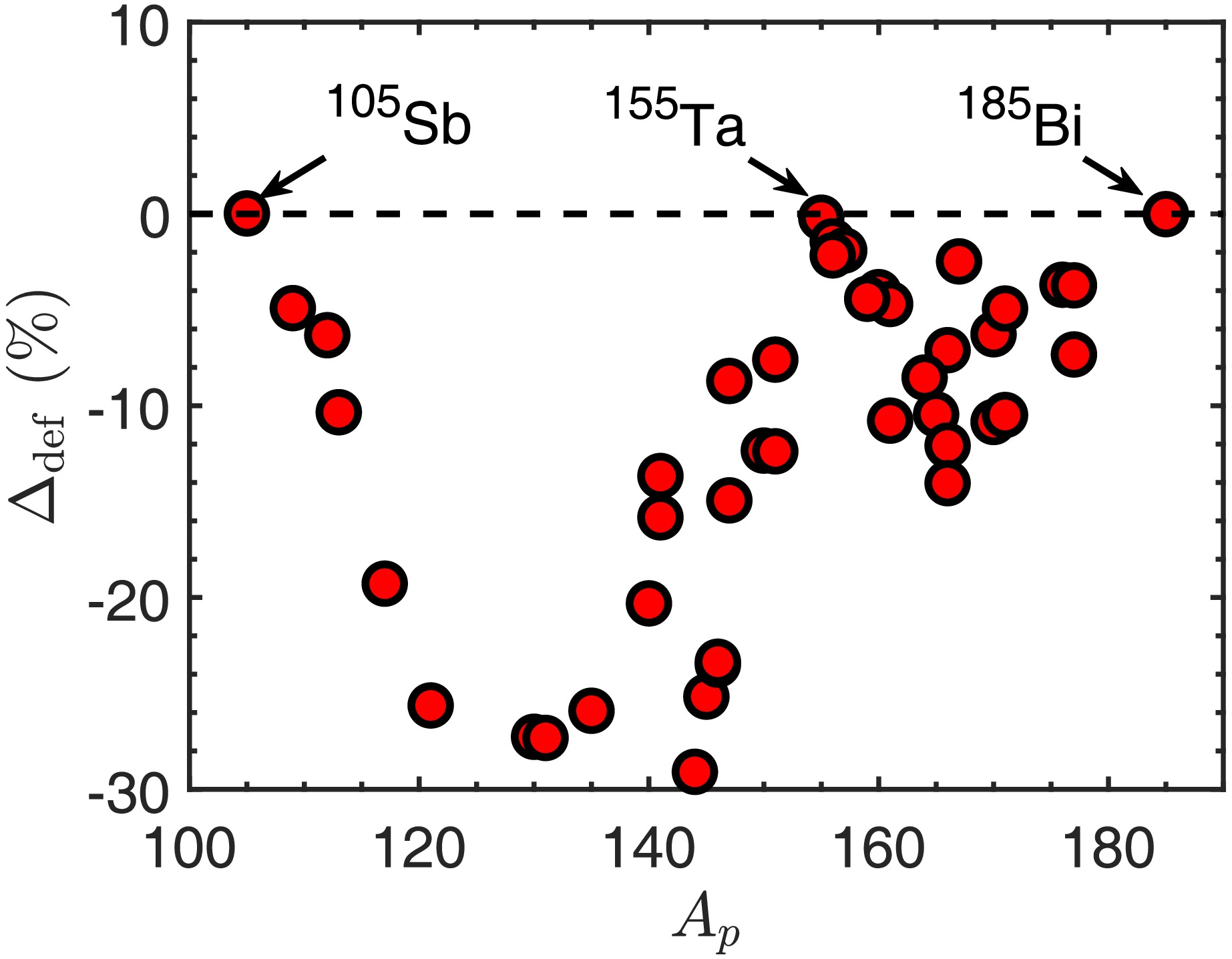

Figure 7.  (color online) Deformation effect on various proton emitters according to Eq. (19). For all proton emitters, negative $ \Delta_{\text{def}} $ implies that both prolate and oblate deformation reduce half-lives.

Subsequently, with nuclear surface polarization taken into account, the parameters $ \tilde{\beta}_2 $and $ \tilde{\beta}_4 $ and results for when polarization is taken into account are shown in Table 3 for those emitters whose polarization parameters are given in Ref. [24]. Here, we use $ S_p^{\text{def,fit}} $ to calculate the half-lives $ \log_{10}T_{1/2}^{\text{pol}} $ with polarization taken into account, and compared the results with those for $ \tilde{\beta}_{2,4}=0 $ to analyze the effect of polarization. The calculations in the previous subsection demonstrate that differences between the experimental and theoretical deformation parameters have a minimal impact on the half-life, and thus, only the theoretical deformation parameters are used in Table 3. The relative variation of the half-life independent to the spectroscopic factor is then defined as follows:

Emitter	$ \tilde{\beta}_2 $	$ \tilde{\beta}_4 $	$\log_{10}T^{\tilde{\beta}_{2,4}=0}_{1/2}\ /\text{s}$	$ \Delta^{\text{pol}}_{\tilde{\beta}_{2,4}=0}({\text{%}}) $	$\log_{10}T^{\text{pol} }_{1/2}\ /\text{s}$	$ \Delta^{\text{pol}} $(%)	$ \overline{a}_N $/fm	$ S_p^{\text{pol,fit}} $	$ \log_{10}T_{1/2}^{\text{pol,fit}}\ /\text{s} $
$ ^{105}\text{Sb} $	0.00089	−0.00154	2.029$ _{-0.459}^{+0.480} $	3.95	2.013$ _{-0.459}^{+0.480} $	0.30	0.74994	0.371	1.992$ _{-0.459}^{+0.480} $
$ ^{109}\text{I} $	0.09182	0.07041	−4.390$ _{-0.053}^{+0.079} $	1.38	−4.370$ _{-0.077}^{+0.059} $	6.05	0.75500	0.137	−4.217$ _{-0.077}^{+0.059} $
$ ^{113}\text{Cs} $	0.10746	0.01397	−5.475$ _{-0.036}^{+0.058} $	−1.90	−5.488$ _{-0.042}^{+0.023} $	−4.86	0.75792	0.070	−5.294$ _{-0.042}^{+0.023} $
$ ^{117}\text{La} $	0.10284	−0.02272	−2.032$ _{-0.161}^{+0.182} $	−4.89	−2.041$ _{-0.183}^{+0.164} $	−6.92	0.76815	0.017	−1.775$ _{-0.183}^{+0.164} $
$ ^{121}\text{Pr} $	0.00738	−0.05577	−2.446$ _{-0.110}^{+0.132} $	3.42	−2.485$ _{-0.156}^{+0.135} $	−5.37	0.76803	0.012	−2.233$ _{-0.156}^{+0.135} $
$ ^{131}\text{Eu} $	−0.02801	−0.07369	−1.733$ _{-0.128}^{+0.114} $	0.04	−1.747$ _{-0.120}^{+0.121} $	−3.04	0.76838	0.007	−1.513$ _{-0.120}^{+0.121} $
$ ^{135}\text{Tb} $	−0.04780	−0.07435	−3.356$ _{-0.073}^{+0.073} $	−7.60	−3.347$ _{-0.055}^{+0.083} $	−5.58	0.76924	0.008	−3.098$ _{-0.055}^{+0.083} $
$ ^{145}\text{Tm} $	−0.08100	−0.00213	−4.974$ _{-0.034}^{+0.045} $	−2.68	−4.963$ _{-0.034}^{+0.056} $	−0.14	0.76255	0.040	−4.729$ _{-0.034}^{+0.056} $
$ ^{147}\text{Tm} $	0.01349	−0.01452	1.055$ _{-0.066}^{+0.067} $	−1.28	1.056$ _{-0.066}^{+0.068} $	−0.96	0.75700	0.272	0.703$ _{-0.066}^{+0.068} $
$ ^{151}\text{Lu} $	0.00070	−0.00119	−0.625$ _{-0.033}^{+0.033} $	−1.08	−0.625$ _{-0.032}^{+0.033} $	−1.06	0.75615	0.304	−0.931$ _{-0.032}^{+0.033} $
$ ^{155}\text{Ta} $	0.00108	−0.00184	−2.524$ _{-0.131}^{+0.133} $	−0.07	−2.524 $ _{-0.131}^{+0.133} $	−0.07	0.75008	0.342	−2.516 $ _{-0.131}^{+0.133} $
$ ^{157}\text{Ta} $	0.00094	−0.00158	−0.261$ _{-0.117}^{+0.118} $	−1.60	−0.261$ _{-0.116}^{+0.118} $	−1.59	0.75138	0.405	−0.414$ _{-0.116}^{+0.118} $
$ ^{161}\text{Re} $	0.00068	−0.00144	−3.243$ _{-0.071}^{+0.071} $	−2.35	−3.231$ _{-0.071}^{+0.071} $	0.40	0.75298	0.158	−3.101$ _{-0.071}^{+0.071} $
$ ^{171}\text{Au} $	0.02322	−0.00585	−4.723$ _{-0.095}^{+0.092} $	2.00	−4.745$ _{-0.095}^{+0.092} $	−2.95	0.75296	0.157	−4.614$ _{-0.095}^{+0.092} $
$ ^{177}\text{Tl} $	0.00800	−0.00863	−1.048$ _{-0.264}^{+0.271} $	−2.66	−1.033$ _{-0.264}^{+0.271} $	0.71	0.75308	0.378	−1.239$ _{-0.264}^{+0.271} $
$ ^{147}\text{Tm}^m $	0.01349	−0.01452	−3.010$ _{-0.055}^{+0.018} $	−1.36	−3.009$ _{-0.054}^{+0.024} $	−1.13	0.75700	0.272	−3.362$ _{-0.054}^{+0.024} $
$ ^{151}\text{Lu}^m $	0.00070	−0.00119	−4.669$ _{-0.097}^{+0.098} $	−1.15	−4.669$ _{-0.097}^{+0.108} $	−1.15	0.75615	0.304	−4.976$ _{-0.097}^{+0.108} $
$ ^{161}\text{Re}^m $	0.00068	−0.00144	−0.640$ _{-0.072}^{+0.073} $	−1.01	−0.640$ _{-0.073}^{+0.073} $	−1.01	0.75298	0.158	−0.510$ _{-0.073}^{+0.073} $
$ ^{171}\text{Au}^m $	0.02322	−0.00585	−3.062$ _{-0.030}^{+0.030} $	−0.81	−3.065$ _{-0.032}^{+0.028} $	−1.35	0.75296	0.157	−2.934$ _{-0.032}^{+0.028} $

Table 3.  Comparison of nuclear surface polarization effect of proton emitters with even-even daughter nuclei. Half-lives $ \log_{10}T^{\text{pol}}_{1/2} $ are calculated with uncertainties arising from decay energies in Ref. [36] based on parameterized polarization using $ \tilde{\beta}_2 $ and $ \tilde{\beta}_4 $ taken from Ref. [24]. Result $ \log_{10}T^{\tilde{\beta}_{2,4}=0}_{1/2} $ is calculated for $ \tilde{\beta}_{2,4}=0 $. Spectroscopic factors are calculated based on our fitting results from Eq. (16), except for the last column, which is based on fitting with the polarization taken into account, using Eq. (18).

the values of which are listed in Table 3. The results show that the average effect of surface polarization defined by Eq. (20) is $ \sum{|{\Delta_i^{\text{pol}}}|}/N=2.35 $%, which indicates that this effect is smaller than the counterpart with deformation. However, when the deformation and polarization in the daughter nuclei are large, $ \Delta_i^{\text{pol}} $ can reach more than 6%, as is the case for $ ^{109}\text{I} $ and $ ^{117}\text{La} $ in Table 3. Compared with the effect of polarization on α decay [25, 26], the proton emitters are relatively less impacted by the polarization, because the nuclear interaction in proton decay is significantly weaker than that in α decay. Hence, it is difficult to directly observe the polarization effect on the half-life of spontaneous proton emission in experiments. To detect polarization, a promising approach is to extract the polar angular distributions of the nuclear surface by comparing the yield ratios of free spectator neutrons to protons in central tip-tip and body-body collisions in relativistic heavy-ion collisions [52, 53]. Another approach is to measure the inverse process of proton emission via proton scattering, and directly observe its angular dependence. In particular, we also show the spectroscopic factor $ S_p^{\text{pol,fit}} $ , obtained by fitting with the polarization taken into account, as expressed in Eq. (18), and the corresponding half-lives in the last two columns.

To measure the errors of the results for different $ S_p $ relative to experimental data, the standard deviation is defined as

As shown in Fig. 8 (a) and (b), considering the half-lives obtained using $ S_p^{\text{RMF}} $ and $ S_p^{\text{def,fit}} $, respectively, the standard deviation is reduced from $ \sigma^{\text{RMF}}=0.620 $ to $ \sigma^{\text{def,fit}}=0.348 $, which proves the feasibility of the relationship expressed by Eq. (16). Furthermore, considering the correlation between spectroscopic factors and deformation and polarization as described in Eq. (18), the standard deviation of the calculated half-lives relative to the experimental data was further reduced from $ \sigma^{\text{def,fit}}=0.345 $ (only for emitters in Table 3) to $ \sigma^{\text{pol,fit}}= $ 0.264, as illustrated in Fig. 8(c), implying the correctness of the relationship of $ S_p $ and polarization.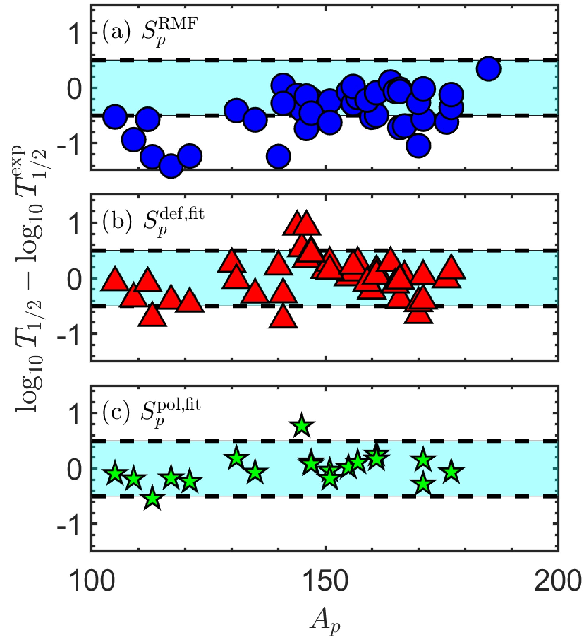

Figure 8.  (color online) Error of calculation relative to experimental results. Spectroscopic factors are taken from (a) RMF theory $ S_p^{\text{RMF}} $ [11], (b) fitting of $ S_p^{\text{def,fit}} $ based on Eq. (16) with only the deformation taken into account, and (c) fitting with polarization $ S_p^{\text{pol,fit}} $ taken into account, based on Eq. (18). Cyan regions represent differences less than $ 0.5 $. Abscissa $ A_P $ represents number of nucleons in parent nuclei.

To conclude, the approximate relationship between $ S_p $ and deformation plus polarization provides a more convenient and accurate method for estimating the spectroscopic factor for proton emitters with deformed and polarized daughter nuclei.

In the subsections above, we performed calculations for various proton emitters that are usually chosen as instances for calculation to verify different kinds of theoretical models in previous research. However, theoretical calculations and discussions related to $ ^{53}\text{Co}^m $, the first proton emitter identified, are not necessarily sufficient compared to calculations and discussions focused on other nuclei. Recently, L. G. Sarmiento, et al. measured the half-life and decay energy of its proton emission into $ ^{52}\text{Fe} $ by experiment [28] and also performed a theoretical calculation based on the barrier-penetration model and R-matrix theory of nuclear reactions, obtaining a successful result. However, their calculation was applicable only for spherical daughter nuclei and neglected the deformation and surface polarization in the theoretical system, so we intend to perform further calculations for this special proton emitter.

Based on the previous experiments on $ ^{53}\text{Co}^m $ to date, there are two decay branches of proton emission in the $ 19/2^+ $ state, which are shown in the decay scheme illustrated in Fig. 9. In the first branch, the daughter nucleus is in the ground state $ 0^+ $, so according to Eq. (9) and Ref. [28], the state of the emitted proton is $n=1, \ell=9, j=19/2$; similarly, the other state of the proton in the other decay channel is $ n=1,\ell=7,j=15/2 $. Other parameters, including branching ratio, decay energy, and half-life, are noted in the scheme.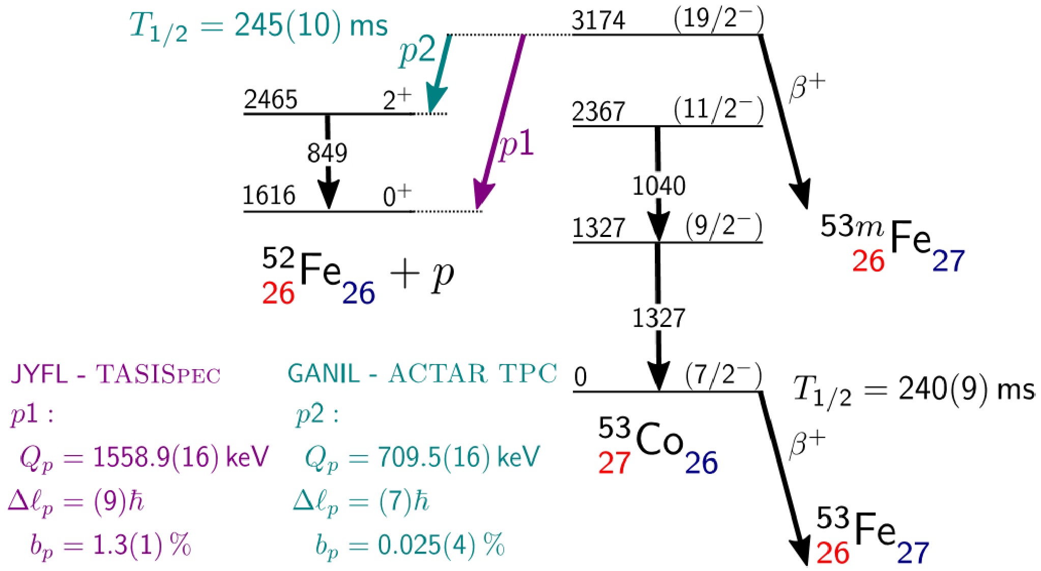

Figure 9.  (color online) Decay scheme of $ ^{53}\text{Co}^m $ from Ref. [28]. Two proton emission branches are denoted by arrows p1 and p2 with corresponding half-lives, branching ratios, and decay energies.

Based on the experimental data, the two proton emission branches are calculated using our theoretical model. The recently observed excited state $ 2^+ $ of daughter nucleus $ ^{52}\text{Fe} $ is not included in Ref. [43, 45], so in our present work, its mass is determined by the mass of $ ^{53}\text{Co}^m $ and the decay energy $ Q_2 $, and its deformation parameters are assumed to be same as those for its ground state because of the absence of theoretical and experimental research. In the future, it is expected that the deformation parameters can be obtained through experiments, such as laser nuclear spectroscopy. To improve the accuracy of our calculation, we use the results of a newer research study for the deformation [54], in which Skyrme interaction with various parameters was used to calculate the deformation. We employ the resulting SKP parameters for the improvement that they offer in pairing matrix elements [54] and their consistency with other research studies [44]. In our calculation, to compare the results of our study with previous theoretical calculation results, we modified the radius for the Coulomb potential and spin-orbit potential in Table 1 to the same parameters as those used for the theoretical calculation program wspot used in Ref. [28]. Other parameters are listed in Table 4, by which we obtain results for the potential and the corresponding quasibound state wave function. It should be noted that compared with other proton emitters, $ ^{53}\text{Co}^m $ has abnormally small spectroscopic factors, which is the reason that we choose to use $ S_p $ calculated by reduced matrix element theoretical calculation in Ref. [28] rather than using our analytic formula Eq. (16) or Eq. (18). Considering the decay branch $ 19/2^-\to0^+ $, Fig. 10 illustrates the quasibound state wave function for spherical daughter nuclei, in which the density distribution is concentrated between the Coulomb barrier and strong centrifugal potential. The deformed Coulomb potential is depicted in detail in Fig. 11 as a function of r and θ separately, with and without the deformation and polarization taken into account; the effect of deformed and polarized Woods-Saxon potential and spin-orbit coupling potential, similar to that shown in Fig. 1, can be observed. The final results in terms of half-lives in two branches using our model are shown in Table 5. The high centrifugal barrier reduces the sensitivity of the half-life to the decay energy, and combined with the relatively lower experimental uncertainty, it leads to a smaller uncertainty in the half-life compared with those for most nuclei listed in Tables 2 and 3. Additionally, compared with the previous theoretical results [28], our results are more consistent with the recent experimental data.

Parameters	Values	Parameters	Values
$ \beta_2 $	$ 0.237 $ [54]	ME($ ^{52}\text{Fe}^m $)	$ -47483.6 (16)\ \text{keV} $
$ \tilde{\beta}_2 $	$ -0.05746 $	$ \tilde{\beta}_4 $	$ -0.00089 $
$ Q_1 $	$ 1558.9(16)\ \text{keV} $	$ Q_2 $	$ 709.5(16)\ \text{keV} $
$ S_p^{p1} $	$ 6.2\times10^{-8} $	$ S_p^{p2} $	$ 1.3\times10^{-7} $

Table 4.  Parameters used in our calculation of $ ^{53}\text{Co}^m $ proton emission. Deformation and polarization parameters are related to the ground state of $ ^{52}\text{Fe} $ in branch p1. Polarization parameters are taken from Ref. [24] of neutron and proton distribution by SkM* functional. ME denotes the mass excess of $ ^{52}\text{Fe}^m $ calculated based on the nuclear mass and decay energy in Ref. [28]. Spectroscopic factors of two branches are taken from the results of reduced matrix element [28].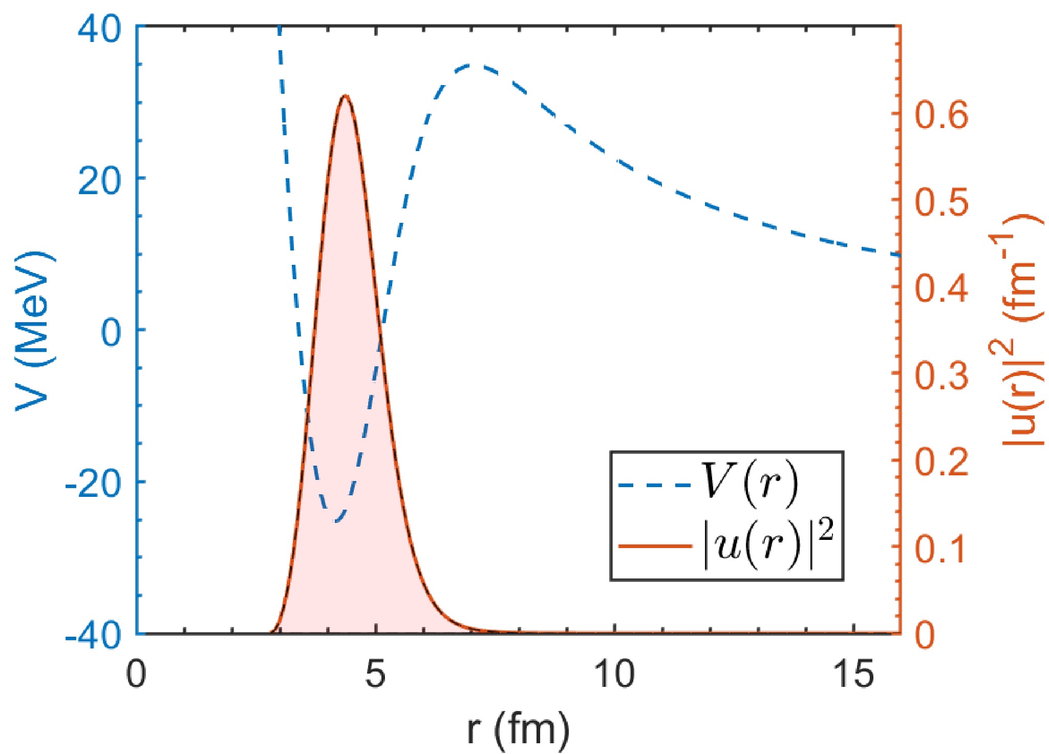

Figure 10.  (color online) Quasibound state of emitted proton in $ ^{53}\text{Co}^m $ [28] of branch $ 19/2^-\to0^+ $. To make the figure more concise, deformation and polarization are not taken into account in this figure.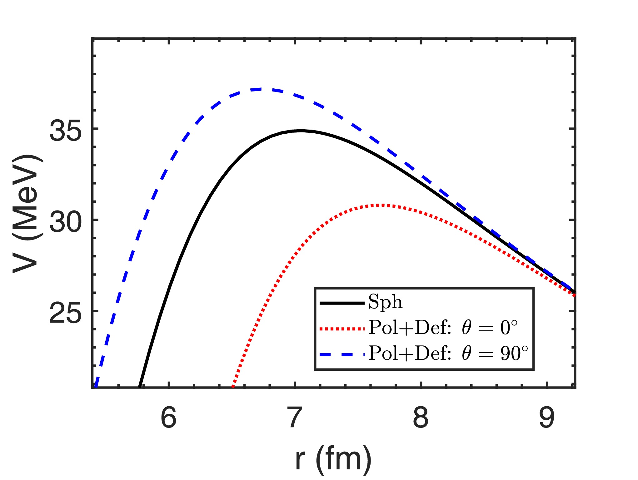

Figure 11.  (color online) Coulomb barrier in $ ^{53}\text{Co}^m $ of branch $ 19/2^-\to0^+ $ combining the deformation and surface polarization of daughter nucleus. Red dotted line represents potential at $ \theta=90^\circ $, and blue dashed line represents potential at $ \theta=0^\circ $.

Results	Reference [28]			This Work
	Exp	Cal		Sph	Def + Pol
$ T_{1/2}^{p1} $ /s	$ 18.8 $$ ^{+1.6}_{-1.6} $	$ 55 $		$ 59.4^{+1.0}_{-1.0} $	$ 43.4^{+0.7}_{-0.7} $
$ T_{1/2}^{p2} $ /s	$ 980 $$ ^{+162}_{-162} $	$ 450 $		713$ ^{+29}_{-28} $	$ 587^{+22}_{-20} $

Table 5.  Theoretical results from our calculations and comparison with experimental results. Superscripts p1 and p2 denote the two branches of proton emission in $ ^{53}\text{Co}^m $ in Fig. 9. Results of calculation and experiment in Ref. [28] are shown in the second and third columns. Fourth to fifth columns present the results of our theoretical model for the spherical daughter nucleus and deformed and polarized daughter nucleus, respectively, with uncertainties introduced by experimental decay energies.

Overall, our calculations show the conspicuously special characteristics of the first discovered proton emitter, $ ^{53}\text{Co}^m $, which is a lighter proton emitter and has extremely high angular momentum and small spectroscopic factor. In comparison to previous studies, our theoretical model that considers deformation and nuclear surface polarization gives more accurate results.

In this work, we reviewed the quantum tunneling model of proton emission through deformed and polarized interaction potential, by which we calculate the half-lives of various proton emitters via distorted wave Born approximation. Based on this theoretical model, we further calculate the effect of deformation and nuclear surface polarization. Polarization destroys the isotropy of diffuseness, changing the geometry of daughter-proton interaction. Results show that polarization will reduce or increase the half-lives of various proton emitters, and the intensity is relatively small and dependent on the values of parameters. In more detail, compared with $ \tilde{\beta}_{2,4}=0 $ case, it can be concluded that for prolate daughter nuclei, positive quadrupole polarization decreases the half-life, and negative quadrupole polarization increases the half-life. By contrast, for oblate daughter nuclei, positive quadrupole polarization increases the half-life.

Sequentially, we also investigate the correlation between the spectroscopic factor and deformation and polarization parameters. The quadratic relationship between the spectroscopic factor and quadrupole deformation and average polarization is proposed as an analytic formula by fitting and validated by comparison with the experimental data. Compared with RMF theory, our fitting that accounts for deformation and nuclear surface polarization gives a more accurate spectroscopic factor and reduces the standard deviation of our theoretical results for the half-lives, suggesting the necessity to consider the surface polarization in calculation.

In addition, based on recent experiments on $ ^{53}\text{Co}^m $, the first observed proton emitter, we calculated the two branches of proton emission, obtaining a result more consistent with the experiment. Our calculations confirm that this proton emitter has an extremely small spectroscopic factor and a relatively long half-life. Results show that our theoretical model that accounts for deformation and polarization gives results that are more consistent with the new experimental data. In the future, more explorations of nuclear surface polarization are anticipated. We hope that these calculations on neutron-deficient nuclei within deformation and polarization can be useful for future research, and that our calculations on $ ^{53}\text{Co}^m $ can expand the insights on special proton emitters.