Gravitational waves and primordial black holes from axion domain walls in level crossing

Gravitational waves (GWs) are among the most effective observational probes of the early Universe [1, 2]. The direct observations of GWs by LIGO [3−5] have made significant advancements in astrophysics and cosmology. Very recently, the pulsar timing array (PTA) projects (NANOGrav [6−8], EPTA [9−11], PPTA [12, 13], and CPTA [14]) released their latest data, which provides strong evidence for the presence of nano-Hertz stochastic GWs. There are various cosmological sources of GWs, such as the primordial amplification of the vacuum fluctuations [15−17], cosmological phase transitions [18, 19], cosmic strings [20−22], domain walls [23−26], and preheating after inflation [27−30]. See, $ \rm e.g. $, Refs. [31−33] for recent reviews of GWs.

After the observations of GWs, primordial black holes (PBHs) have recently gained significant interest as attractive cold dark matter (DM) candidates. There are several scenarios for PBH formation in the early Universe, such as the large density fluctuations produced during inflation [34−37], cosmological phase transitions [38−41], and collapse of the false vacuum bubbles [42−44]; cosmic strings [45−47]; domain walls [48−51]; and the post-inflationary scalar field fragmentations [52−54]. See also, $ \rm e.g. $, Refs. [55−57] for recent reviews of the PBHs.

Here, we consider the domain wall as a cosmological source of GWs and PBHs. Domain walls are two-dimensional topological defects that may arise in the early Universe, involving the spontaneous breakdown of a discrete symmetry [58, 59]. For long-lived domain walls, their evolution with cosmic expansion is slower than that of radiation or matter, and they will eventually dominate the total energy density of the Universe, which conflicts with the standard cosmology [60]. This is the so-called domain wall problem. To avoid such a cosmological catastrophe, one can make the domain walls disappear or prevent their formation before dominating the Universe [61−63].

The GWs emitted by domain wall annihilation can be characterized by their peak frequency and peak amplitude, where the former is determined by the domain wall annihilation time and the latter is determined by the energy density of the domain walls [64−66]. Here, we focus our attention on the GW emission from domain wall annihilation, especially axion domain walls [67−85]. In addition, during the annihilation, the closed domain walls could shrink to the Schwarzschild radius and then collapse into the PBH. In this case, PBHs will form when this Schwarzschild radius is comparable to the cosmic time. See also, $ \rm e.g. $, Refs. [83−94] for recent PBH mechanisms with the framework of the QCD axion or axion-like particle (ALP).

In this paper, we investigate the nano-Hertz GW emission and massive PBH formation from the light QCD axion scenario discussed in Ref. [95]. The basic idea is to consider the axion domain wall formation from the level crossing induced by the light $ Z_{\mathcal N} $ QCD axion. In the $ Z_{\mathcal N} $ axion scenario [96], the $ \mathcal N $ mirror worlds are nonlinearly realized by the axion field under a $ Z_{\mathcal N} $ symmetry, one of which is the Standard Model (SM) world. The $ Z_{\mathcal N} $ axion with reduced-mass can both solve the strong CP problem with $ \mathcal N\geqslant3 $ [97] and account for the DM through the trapped+kinetic misalignment mechanism [98, 99]. Considering the interaction between the $ Z_{\mathcal N} $ axion and ALP, the cosmological evolution of single/double level crossings will occur if there is a non-zero mass mixing between them [95, 100]. In this work, we consider a more general case in the mixing, where the heavy and light mass eigenvalues do not necessarily have to coincide with the axion masses, and there is a hierarchy between the two axion decay constants. To form the domain walls in this scenario, the axions should start to oscillate slightly before the level crossing, and the initial oscillation energy density should be large to climb over the barrier of potential [101].

To avoid the unacceptable cosmological catastrophe, the domain walls must annihilate before dominating the Universe. Then, we investigate the GWs emitted by the domain wall annihilation and show the predicted GW spectra, determined by their peak frequency and peak amplitude. For model parameters with the benchmark values, we have the predicted GW spectrum with the peak frequency $f_{\rm peak}\sim 0.2~ \rm nHz$ and peak amplitude $ \Omega_{\rm GW}h^2\sim 5\times 10^{-9} $, which will be observable in future GWs detectors, such as the PTA projects. Finally, we investigate the PBH formation from the domain wall collapse. We consider the domain wall collapse in an approximately spherically symmetrical manner. PBHs will form when the ratio of Schwarzschild radius to cosmic time is close to 1, leading to $ \mathcal{O}(10^5-10^8) M_\odot $ (in solar mass $ M_\odot $) massive PBHs as a small fraction $ f_{\rm PBH}\sim 10^{-5} $ of the cold DM. In this regard, we find that these PBHs may also account for the seeds of supermassive black holes (SMBHs) at high redshift. See Fig. 1 for the main cosmic temperatures related to this work.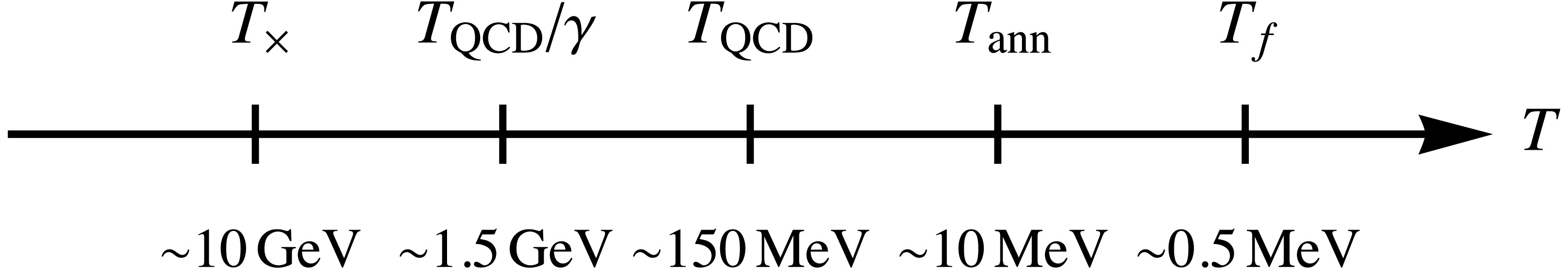

Figure 1.  Main cosmic temperatures related to this work, where $ T_\times $ represents the level crossing temperature, $ T_{\rm QCD} $ represents the QCD phase transition critical temperature, $ T_{\rm ann} $ represents the domain walls annihilation temperature, $ T_f $ represents the PBH formation temperature, and $ \gamma\in(0,1) $ is a temperature parameter. The temperature is decreasing from left to right. Note that the ticks are shown just for illustrative purposes. See the text for more details.

The remainder of this paper is organized as follows. In Section II, we introduce the light QCD axion scenario and discuss domain wall formation and annihilation. In Section III, we investigate the GWs emitted by the domain wall annihilation and the PBH formation from the domain walls collapse. Finally, conclusions are given in Section IV.

In this section, we first introduce the light QCD axion and resulting axion level crossing. Then, we discuss the domain wall formation and annihilation.

In the light $ Z_{\mathcal N} $ QCD axion scenario [96], the $ \mathcal N $ mirror and degenerate worlds that are nonlinearly realized by the axion field under a $ Z_{\mathcal N} $ symmetry can coexist with the same coupling strengths as in the SM:

where $ \mathcal L_{{\rm SM}_k} $ represents the copies of the SM total Lagrangian excluding the topological term $ G_k \widetilde{G}_k $, $ \alpha_s $ is the strong fine structure constant, and ϕ and $ f_a $ are the $ Z_{\mathcal N} $ axion field and decay constant, respectively. In the large $ \mathcal N $ limit, the temperature-dependent $ Z_{\mathcal N} $ axion mass is given by [97, 98]

The zero-temperature $ Z_{\mathcal N} $ axion mass $ m_{a,0} $ and defined mass $ m_{a,\pi} $ are

where $ \gamma\in(0,1) $ is a temperature parameter, $ T_{\rm QCD}\simeq $ 150 MeV is the QCD phase transition critical temperature, $ b\simeq4.08 $ is an index, $ m_\pi $ and $ f_\pi $ are the mass and decay constant of the pion, respectively, and $ z\equiv m_u/m_d\simeq0.48 $ is the ratio of up ($ m_u $) to down ($ m_d $) quark masses. The level crossing can take place at the temperature $ T_\times $ in the interaction between the $ Z_{\mathcal N} $ axion and ALP (ψ) with the potential [95]

with the overall scales

where $ m_A $ and $ f_A $ are the ALP mass and decay constant, respectively, n is a positive integer, and n and $ \mathcal N $ are domain wall numbers. Through the mass mixing matrix derived from Eq. (5), we can obtain the heavy (h) and light (l) mass eigenvalues $ m_{h,l} $, which are temperature-dependent. See Fig. 2 for an illustration of the level crossing; in the following, we will consider this case.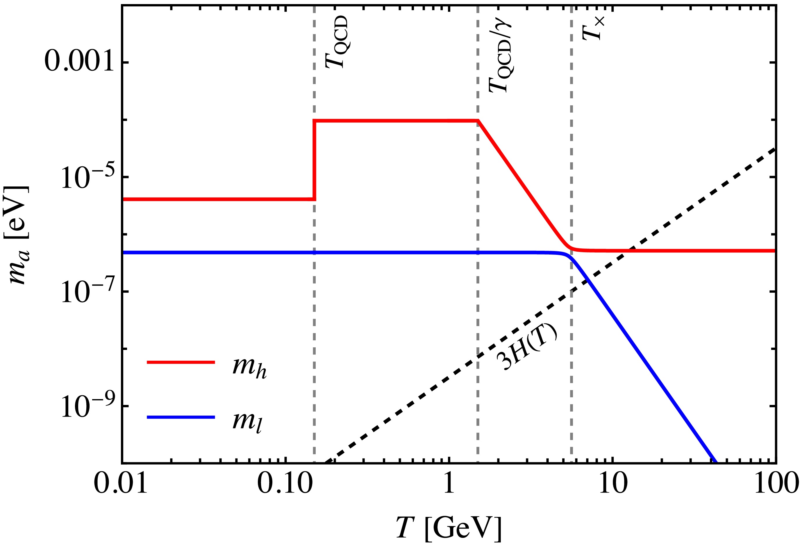

Figure 2.  (color online) Temperature-dependent mass eigenvalues $ m_{h,l} $ as functions of the cosmic temperature T. The red and blue solid lines represent $ m_h $ and $ m_l $, respectively. The black dashed line represents the Hubble parameter $ H(T) $.

Note however that in this work, the heavy and light mass eigenvalues do not necessarily have to coincide with the axion masses, which is somewhat different from the case in Ref. [95]. In general, there is a hierarchy between the two axion decay constants [102, 103]. Considering two physical fields μ and ξ, in which the first one is the linear combination in the first term of Eq. (5) and second one is the orthogonal combination, with

then the potential in terms of the physical fields can be written as

with the effective axion decay constants $ f_\mu $ and $ f_\xi $

In this subsection, we briefly discuss the axion domain wall formation in this scenario. The domain wall formation from the canonical level crossing case was studied in Ref. [101]. It was shown that the formation of domain walls from the level crossing in the axiverse is a common phenomenon. The onset of axion oscillations is considered slightly before the level crossing temperature $ T'_\times $. In the case the initial axion oscillation energy density is sufficiently large to climb over the barrier of potential, the axion dynamics therefore show a chaotic run-away behavior (also called the axion roulette), which is considered to be accompanied by the domain wall formation.

In our scenario, we have a similar consideration that the axions start to oscillate slightly before the level crossing

where $ T_1 $ is the axion oscillation temperature given by $ m_{h,l}(T)=3H(T) $, with the Hubble parameter

where $ g_* $ is the number of effective degrees of freedom of the energy density, and $ m_{\rm Pl}\simeq 2.44\times10^{18}\, \rm GeV $ is the reduced Planck mass. Note that here the level crossing occurs earlier than the canonical case with

Then, another condition for axion domain wall formation is that the oscillation energy density in the light mass eigenvalue $ m_l $ should be larger than the barrier of potential

where the subscript "1" corresponds to $ T_1 $. Because no cosmic strings are formed, the domain walls without cosmic strings are stable in a cosmological time scale.

Then, we discuss the domain wall annihilation. After formation, we consider that the dynamics of domain walls is dominated by the tension force. In the scaling regime, the evolution of walls can be described by the scaling solution [104−107]. In this case, the energy density of domain walls evolves as

where $ \mathcal{A}\simeq 0.8 \pm 0.1 $ is a scaling parameter obtained from the numerical simulations, and $ \sigma_{\rm wall} $ is the tension of domain walls

where we have defined the parameters

Due to the slower evolution of domain walls with the cosmic expansion compared to radiation or matter, the walls will eventually dominate the Universe, which conflicts with the standard cosmology. Therefore, to avoid the domain wall problem, they must annihilate before dominating the Universe. In general, one can introduce an additional small energy difference – "bias" – between the different vacua to drive the domain walls towards their annihilation. In our scenario, the domain walls will become unstable and annihilate due to the natural bias term

where we have defined a bias parameter $ \Lambda_b $, and δ is a CP phase, which should not spoil the Peccei-Quinn (PQ) solution to the strong CP problem. Note that the scale $ \Lambda_b $ should be several orders of magnitude smaller than the QCD scale, but too small a $ \Lambda_b $ may lead to the long-lived domain walls that overclose the Universe.

Then, the resulting volume pressure $ p_V\simeq \Lambda_b^4 $ accelerates the domain walls towards the higher energy adjacent vacuum, converting the higher energy vacuum into the lower energy vacuum. The wall annihilation becomes significant when the pressure produced by the tension $ p_T\simeq\rho_{\rm wall} $ is comparable to the volume pressure. By taking $ p_T\simeq p_V $, we have

where the domain wall annihilation time $ t_{\rm ann} $ is given by $ H(T_{\rm ann})=1/(2t_{\rm ann}) $, corresponding to the domain walls annihilation temperature

Here, we take the benchmark values as $ \zeta=0.1 $, $ \eta=0.1 $, $ f_a=10^{16}\, \rm GeV $, and $\Lambda_b=1~ \rm MeV$. In Fig. 3, we show the annihilation temperature $ T_{\rm ann} $ as a function of the $ Z_{\mathcal N} $ axion decay constant $ f_a $. The red and blue lines correspond to the parameters $\Lambda_b=1~ \rm MeV$ and $0.5~ \rm MeV$, respectively. The other parameters are taken as the benchmark values. We note that $ T_{\rm ann} $ is below the QCD phase transition critical temperature. Additionally, the domain wall annihilation should be before the Big Bang Nucleosynthesis (BBN) epoch to avoid strong constraints, $ \rm i.e. $, $T_{\rm ann} > T_{\rm BBN}\simeq $ 0.1 MeV. Then, we have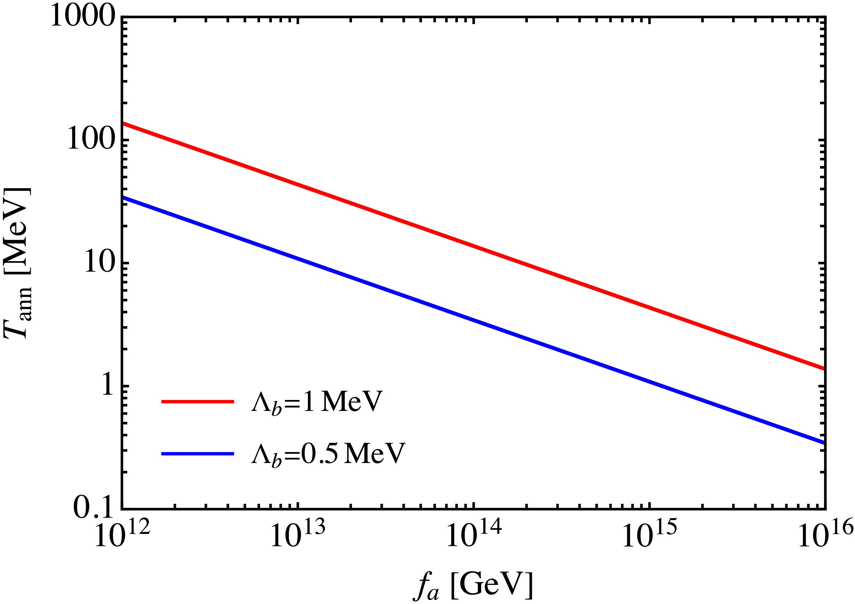

Figure 3.  (color online) Domain wall annihilation temperature $ T_{\rm ann} $ as a function of the $ Z_{\mathcal N} $ axion decay constant $ f_a $. The red and blue lines represent $\Lambda_b=1~ \rm MeV$ and $0.5~ \rm MeV$, respectively. Here, we take the benchmark values as $ \zeta=0.1 $ and $ \eta=0.1 $.

Fig. 4 shows the bias parameter $ \Lambda_b $ constrained by BBN in the $ \{f_a, \, \Lambda_b\} $ plane with the red shadow region.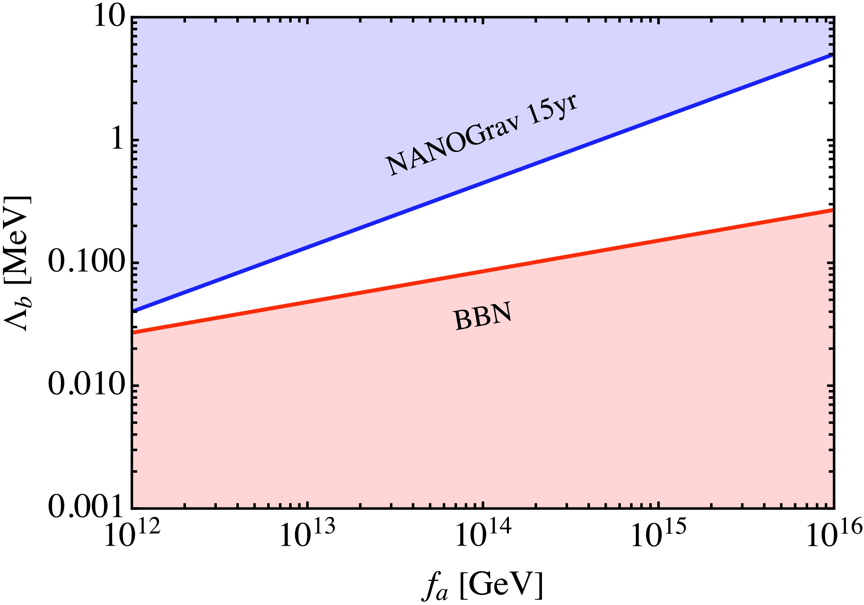

Figure 4.  (color online) Constraints of BBN and NANOGrav 15-year dataset in the $ \{f_a, \, \Lambda_b\} $ plane. The red shadow region represents the constraint set by BBN. The blue shadow region represents that the predicted GW spectra cannot explain the NANOGrav 15-year dataset, as detailed in the text. Here, we set $ \zeta=0.1 $ and $ \eta=0.1 $.

In this section, we investigate the GW emission from the domain wall annihilation and PBH formation from the domain wall collapse.

The GWs emitted by the domain wall annihilation can be characterized by their peak frequency and peak amplitude. The GW peak frequency corresponds to the Hubble parameter at the domain wall annihilation time:

where $ f=\kappa/(2\pi) R(t) $ is the frequency with the comoving wavenumber κ, and $ R(t) $ is the scale factor of the Universe. Considering the redshift of the peak frequency due to the subsequent cosmic expansion, we can obtain the peak frequency at the present time $ t_0 $ as

The GW spectrum at the cosmic time t can be described by

where $ \rho_c(t) $ is the critical energy density. Then, the GW peak amplitude at the domain wall annihilation time is given by [108]

where $ \tilde{\epsilon}_{\rm gw}\simeq 0.7 \pm 0.4 $ is an efficiency parameter, and G is Newton’s gravitational constant. We also have the peak amplitude at present

where $ \Omega_{\rm rad} h^2 \simeq 4.15\times 10^{-5} $ is the density parameter of radiation at present, $ h\simeq 0.68 $ is the reduced Hubble parameter, and $ g_{*s} $ is the number of effective degrees of freedom of the entropy density. Using Eqs. (24) and (27), the present GW spectrum is finally given by

which can be described by a piecewise function that evolves as $ \Omega_{\rm gw}h^2\propto f^3 $ for the low frequencies and $ \Omega_{\rm gw}h^2\propto f^{-1} $ for the high frequencies [66].

The predicted GW spectra emitted by the axion domain wall annihilation in our scenario are shown in Fig. 5. There are four parameters (ζ, η, $ f_a $, and $ \Lambda_b $) that significantly determine the GW peak frequency and peak amplitude. As discussed before, we take these benchmark values as $ \zeta=0.1 $, $ \eta=0.1 $, $f_a=10^{16}~ \rm GeV$, and $\Lambda_b=1~ \rm MeV$, corresponding to the red solid line in the panels. The blue and green solid lines are produced by changing only one parameter each time with $ \zeta=0.02 $, $ \eta=0.02 $, $f_a= 2\times10^{15}~ \rm GeV$, and $\Lambda_b=5~ \rm MeV$. We find that η and $ \Lambda_b $ have a significantly greater impact on the GW spectra than ζ and $ f_a $. Note that the lines corresponding to the changes of the parameters ζ and $ f_a $ have the same distribution; this is because they are degenerate in the calculations of the domain wall annihilation temperature and the GW spectrum. The results of the recently published NANOGrav 15-year dataset [6, 7] and other experimental sensitivities (SKA [109], TianQin [110], Taiji [111], and LISA [112]) in the plot region are also shown for comparisons. We find that the predicted nano-Hertz GW spectra in this scenario can be tested by the current and future PTA projects.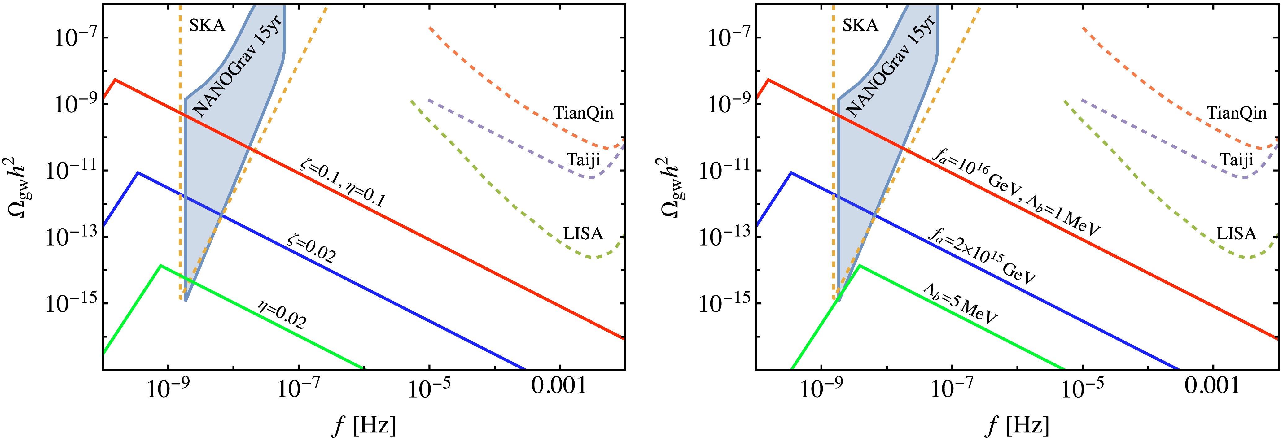

Figure 5.  (color online) Predicted GW spectra $ \Omega_{\rm gw}h^2 $ as a function of frequency f, with parameter uncertainties of ζ, η, $ f_a $, and $ \Lambda_b $. The red solid lines represent the result with the benchmark values $ \zeta=0.1 $, $ \eta=0.1 $, $ f_a=10^{16}\, \rm GeV $, and $ \Lambda_b=1\, \rm MeV $. Left: The blue and green solid lines represent the results with $ \zeta=0.02 $ and $ \eta=0.02 $, respectively. Right: The blue and green solid lines represent the results with $ f_a=2\times10^{15}\, \rm GeV $ and $ \Lambda_b=5\, \rm MeV $, respectively. The result of the NANOGrav 15-year dataset [6, 7] and other experimental sensitivities (SKA [109], TianQin [110], Taiji [111], and LISA [112]) in this plot region are also shown.

Meanwhile, according to the BBN bound and NANOGrav 15-year dataset, we find a roughly allowed region for the bias parameter, $ {0.3~\rm MeV}\lesssim\Lambda_b\lesssim {5~\rm MeV} $. Note that this is obtained when other parameters (ζ, η, and $ f_a $) are taken as the corresponding benchmark values. See also Fig. 4 with the blue shadow region in the $ \{f_a, \, \Lambda_b\} $ plane. The blue line is estimated using the two points where $ f_a $ equals $10^{12}~ \rm GeV$ and $10^{16}~ \rm GeV$, at which the predicted GW spectra barely reach the NANOGrav 15-year dataset. Then, the shadow region, within the parameter space characterized by a larger $ \Lambda_b $, indicates that the corresponding peak frequency and amplitude of GWs cannot be used to explain the observational data. Moreover, due to the large parameter degrees of freedom in the model, and because there may be constraints on ζ and η from the conditions for the level crossing to occur [95], we do not show the concrete QCD axion (or ALP) properties ($ m_a $, $ f_a $) from the GWs measurement in this work.

In this subsection, we investigate the PBH formation from the domain wall collapse. During the annihilation, the closed domain walls could shrink to the Schwarzschild radius and collapse into the PBHs [86]. Here, we consider the domain wall collapse in an approximately spherically symmetric manner [84, 85].

The Schwarzschild radius $ R_S(t) $ at the cosmic time t is given by $ R_S(t)=2M(t)/M_{\rm Pl}^2 $, where $ M_{\rm Pl}=1.22\times10^{19}\, \rm GeV $ is the Planck mass, and $ M(t) $ is the mass of the closed domain walls at the time t

The condition for PBHs to form is that the ratio of $ R_S(t) $ to t is close to 1, $ \rm i.e. $,

At the domain wall annihilation time $ t_{\rm ann} $, the wall tension pressure is comparable to the volume pressure. Because $ V_{\rm bias}\simeq \mathcal{A} \sigma_{\rm wall}/t_{\rm ann} $ given by $ p_T\simeq p_V $, we obtain the mass $ M(t) $ and ratio $ p(T) $ at $t_{\rm ann}: M(t_{\rm ann}) \simeq 16/3 \pi V_{\rm bias} t_{\rm ann}^3$ and $ p(T_{\rm ann})\simeq 30 V_{\rm bias} / (\pi^2 g_*(T_{\rm ann}) T_{\rm ann}^4) $, respectively. After the time $ t_{\rm ann} $, because the tension pressure decreases with time while the volume pressure remains constant, the volume contribution to the density will rapidly become dominated. Then, the mass $ M(t) $ and ratio $ p(T) $ can be given by $ M(t)\simeq 4/3 \pi V_{\rm bias} t^3 (1+3 t_{\rm ann}/t) $ and $p(T)\simeq p(T_{\rm ann})/4 (t/t_{\rm ann})^2 (1+3 t_{\rm ann}/t)$, respectively. Here, the term $ t_{\rm ann}/t $ can be neglected for $ t\gg t_{\rm ann} $. As mentioned before, the PBH formation will occur when the ratio $ p(T_f)\sim 1 $. Thus, we have

where $ T_f $ is the PBH formation temperature. Then, the corresponding PBH mass is given by

and the temperature $ T_f $ can also be characterized as

We show the temperature $ T_f $ as a function of the bias parameter $ \Lambda_b $ in Fig. 6. For the benchmark value $ \Lambda_b= $ 1 MeV, we have $ T_f\simeq 0.5\, \rm MeV $. Note that $ T_f $ is only determined by the term $ V_{\rm bias} $ ($ \Lambda_b $), or the PBH mass $ M_{\rm PBH} $.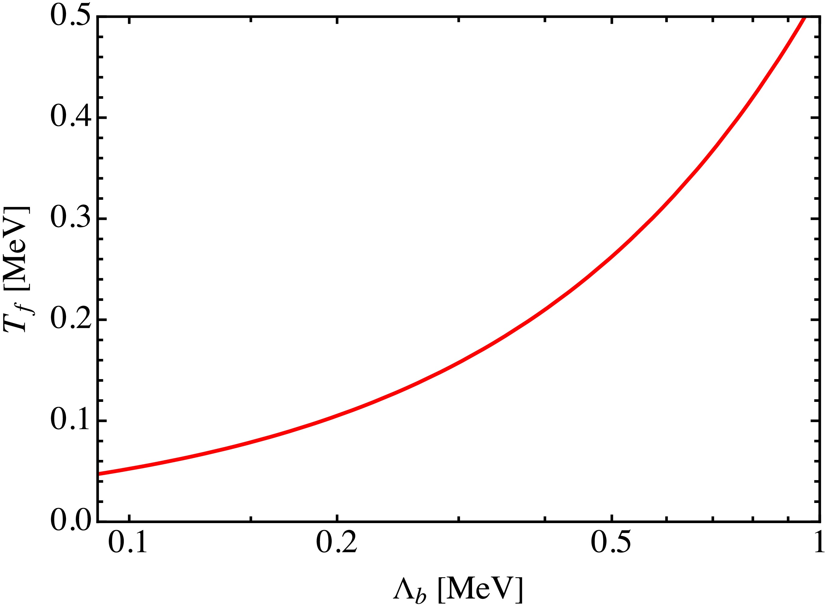

Figure 6.  (color online) The PBH formation temperature $ T_f $ as a function of the bias parameter $ \Lambda_b $.

Then, we estimate the PBH fraction of the total DM energy density in this scenario. The PBH energy density at the formation temperature is given by $\rho_{\rm PBH}(T_f)\simeq p^\beta(T_f) \rho_{\rm wall}(T_f)$, where β is a positive factor representing the small deviations from the spherically symmetric collapse. Because we have $p(T_f)\sim 1 \Rightarrow p^\beta(T_f)\sim 1$ and the domain wall energy density after annihilation evolves as $ \rho_{\rm wall}(T)/\rho_{\rm wall}(T_{\rm ann})\simeq (T/T_{\rm ann})^\alpha $, the PBH fraction can be described by $f_{\rm PBH}\simeq (T_f/T_{\rm ann})^\alpha \rho_{\rm wall} (T_{\rm ann})/ \rho_{\rm DM}(T_f)$, where α is a positive parameter between approximately 5 and 20 [113]. Finally, the PBH fraction is given by

where $ T_0 $ is the present cosmic microwave background (CMB) temperature, $ \rho_R $ is the radiation energy density, and $ \rho_{\rm DM} $ is the DM energy density. We show the estimated PBH fraction $ f_{\rm PBH} $ as a function of the PBH mass $ M_{\rm PBH} $ in Fig. 7. The other limits in this plot region from the CMB [114], X-ray binaries (XB) [115], dynamical friction (DF) [55], and large-scale structure (LSS) [116] are also shown. Because in our model there are four parameters (ζ, η, $ \Lambda_b $, and $ f_a $) that determine the domain wall annihilation temperature $ T_{\rm ann} $, here, we only show the PBH fraction with the parameters $ T_{\rm ann} $ and α in the figure. We take these typical values as $ T_{\rm ann}=$ 10 MeV and $ 1~ \rm MeV $, corresponding to the left and right panels, respectively, and take $ \alpha=5 $, 10, and 20, corresponding to the red, blue, and black dashed lines, respectively. Because we only take several typical values of the parameter α, more accurate discussions about α from the simulations are required [113]. We find that the PBHs in the mass range of $ 10^5 \, M_\odot \lesssim M_{\rm PBH} \lesssim 10^8 \, M_\odot $ could potentially form in our scenario and account for a small fraction $ f_{\rm PBH}\sim 10^{-5} $ of the cold DM.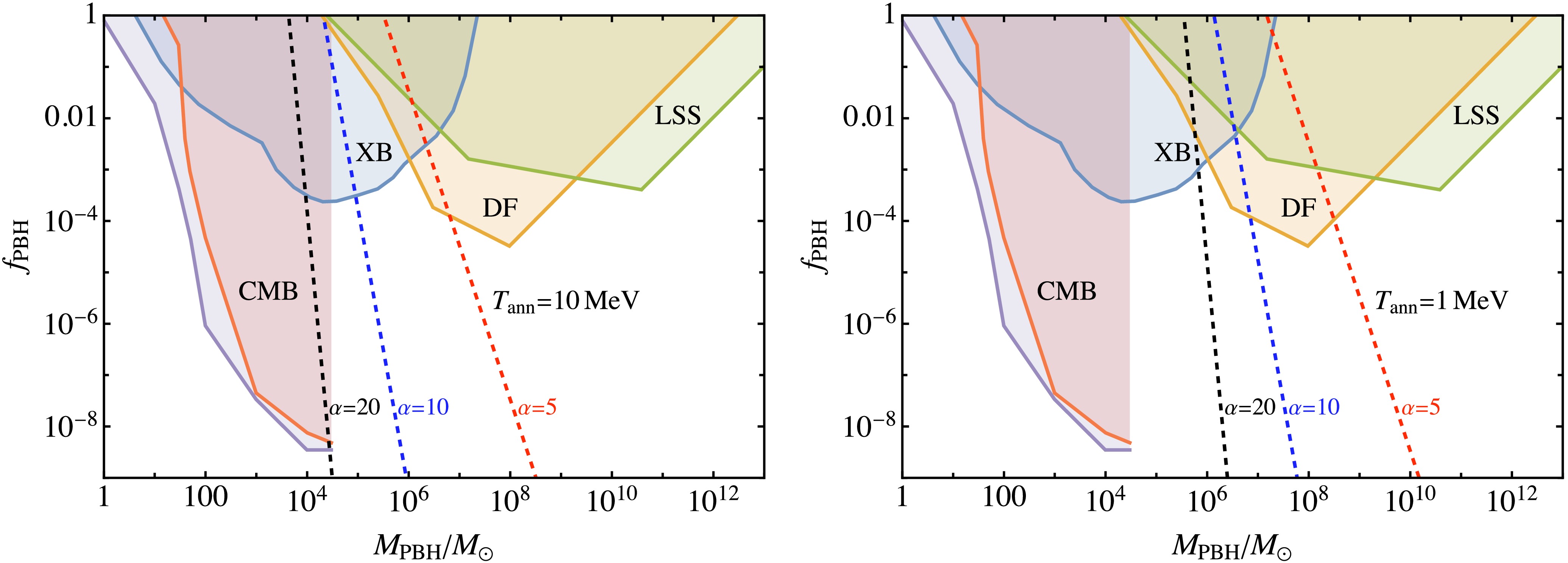

Figure 7.  (color online) Estimated PBH fraction $ f_{\rm PBH} $ as a function of the PBH mass $ M_{\rm PBH} $ (in the solar mass $ M_\odot $). Left: we set $T_{\rm ann}=10~ \rm MeV$. Right: we set $T_{\rm ann}=1~ \rm MeV$. The red, blue, and black dashed lines represent the PBH fraction with the typical values $ \alpha=5 $, 10, and 20, respectively. The other limits (shadow regions) are taken from the accretion limits from the CMB anisotropies measured by Planck (CMB, with two bounds) [114], the accretion limits from the X-ray binaries (XB) [115], dynamical limits from the infalling of halo objects due to the dynamical friction (DF) [55], and large-scale structure (LSS) limits from the various cosmic structures [116].

Furthermore, we also find that these PBHs may account for the seeds of SMBHs at high redshift. The SMBHs with a mass range of $ \mathcal{O}(10^6-10^9)\, M_\odot $ are commonly found in the center of galaxies [117−119]. However, their origin is not yet clear. One may consider their formation from the stellar black holes through accretion and mergers, but it is difficult to account for the SMBHs at high redshift $ z\sim 7 $. Another scenario is considering the PBHs as their primordial origin [120, 121]. Due to the efficient accretion of matter on the massive seeds and mergings, those $ \mathcal{O}(10^4-10^5)\, M_\odot $ PBHs could subsequently grow up to $ \mathcal{O}(10^9)\, M_\odot $ SMBHs. Therefore, the massive PBHs produced in our scenario are natural candidates for the seeds of SMBHs.

In summary, in this work, we investigated the GW emission and PBH formation from the light QCD axion scenario. We first introduced the light QCD axion and resulting axion level crossing. Then, we discussed the domain wall formation from the level crossing and their annihilation. Finally, we investigated the cosmological implications, including the nano-Hertz GW emission from the domain wall annihilation and the massive PBH formation from the domain wall collapse.

We consider the axion domain wall formation from the level crossing induced by the mass mixing between the light $ Z_{\mathcal N} $ QCD axion and ALP, leading to the wall formation before the QCD phase transition. A more general mixing case in which the heavy and light mass eigenvalues do not necessarily have to coincide with the axion masses is considered, and there is a hierarchy between the two axion decay constants. The conditions for domain wall formation are that the axions should start to oscillate slightly before the level crossing, and the initial axion oscillation energy density should be large to climb over the barrier of potential. To avoid cosmological catastrophe, the domain walls must annihilate before dominating the Universe. Then, we focus our attention on the GW emission and PBH formation. The GWs emitted by the domain wall annihilation are determined by their peak frequency and peak amplitude. We present the predicted GW spectra with the peak frequency $f_{\rm peak}\sim 0.2~ \rm nHz$ and peak amplitude $ \Omega_{\rm GW}h^2\sim 5\times 10^{-9} $, which can be tested by current and future PTA projects. During the domain wall annihilation, the closed walls could shrink to the Schwarzschild radius and collapse into the PBHs when this radius is comparable to the cosmic time. Finally, we show the estimated PBH fraction and find that the PBHs in the mass range of $ 10^5 \, M_\odot \lesssim M_{\rm PBH} \lesssim 10^8 \, M_\odot $ could potentially form in this scenario and account for a small fraction $ f_{\rm PBH}\sim 10^{-5} $ of the cold DM. Furthermore, it is natural to consider the SMBH formation from these PBHs.