Modification of the Sommerfeld effect due to coannihilator decays

The cold dark matter (DM) density of the Universe has been determined by observation to a percent level accuracy, $ \Omega_c h^2 = 0.120\pm0.001$ [1]. It is the only precise quantity we know about DM, and it certainly deserves thorough investigations. One way to obtain this value in theory is through the thermal freeze-out mechanism [2, 3]. This mechanism is attractive because it has successfully helped to explain two other important relics of our Universe — the cosmic microwave background and the light elements from Big-Bang nucleosynthesis.

During freeze-out, typical velocities of cold DM particles are non-relativistic. If there is some long-range interaction between DM particles, the two-body wave function of an annihilating DM pair is modified from a plane wave, and therefore, the annihilation cross section and consequently the DM thermal relic abundance are affected. This is the Sommerfeld effect [4, 5]. Roughly speaking, the annihilation cross section is the product of the so called Sommerfeld factor and the bare annihilation cross section. The latter is calculated through the usual relativistic quantum field theory approach using plane wave functions. The Sommerfeld factor can be obtained in the non-relativistic quantum mechanics framework by solving for the scattering wave function of a particle moving in a long-range potential. It is greater than 1 (i.e., Sommerfeld enhancement) if the potential is attractive, while it is less than 1 (i.e., Sommerfeld suppression) if the potential is repulsive. A stronger attractive or repulsive potential gives a more significant Sommerfeld enhancement or suppression, as it results in a larger modification of the scattering wave function relative to the plane wave function. A small relative velocity $ v_{\rm rel} $ between the two annihilating particles is another indispensable ingredient in achieving a significant Sommerfeld enhancement or suppression. This can be understood intuitively. A smaller $ v_{\rm rel} $ means that the potential can act on the annihilating particles for a longer time before they meet and annihilate, such that a larger accumulation of the modification of the two-body wave function can be achieved. For example, at small $v_{\rm rel}$, the s-wave Sommerfeld factor for a Coulomb-like potential $ V(r) = - \dfrac{\alpha}{r} $ of an infinite range is approximately ${2 \pi \alpha}/{v_{\rm rel}}$ for an attractive case ($ \alpha > 0 $), and it is approximately $-\dfrac{2 \pi \alpha}{v_{\rm rel}} \mathrm{e}^{\frac{2 \pi \alpha}{v_{\rm rel}}}$ for a repulsive one ($ \alpha < 0 $). The Sommerfeld effect on DM thermal relic abundance calculations has been well-studied (see, e.g., [6, 7]). Also, Sommerfeld factors may be crucial in explaining DM indirect detection results (see, e.g., [8, 9]).

Another important add-on during freeze-out is coannihilation [10]. Some particle species (i.e., coannihilators), which are slightly heavier than DM particles, freeze out together with the latter. Through scatterings and (inverse-)decays, coannihilators and DM particles can interconvert to each other. Consequently, the ratio of their number densities equals the equilibrium value at temperatures during freeze-out if the interconversion rate is larger than the Hubble expansion rate. Depending on the relative sizes of the DM-DM, DM-coannihilator, and coannihilator-coannihilator (co)annihilation cross sections, the mass difference between the coannihilator and DM particle, and their degrees of freedom, the DM relic abundance can be smaller or larger than if no coannihilator species exist [11]. Coannihilation is a feasible and sometimes unavoidable feature in many theories beyond the Standard Model (BSM), including scenarios in supersymmetry [12, 13] and Universal Extra Dimensions [14, 15]. Various coannihilation models in DM searches have also been extensively studied (see, e.g., [16]).

If there is some long-range interaction between coannihilators, the Sommerfeld effect of annihilating coannihilators must be taken into account in the calculation of DM thermal relic abundance. In fact, compared to DM particles, it is more common to have long-range interactions between coannihilators. For example, coannihilators can be electrically and/or color charged [17−20], but the DM usually cannot be. Long-range interactions felt by dark sector particles can arise not only from Standard Model gauge and Higgs interactions but also from the exchanges of new gauge bosons or scalars in BSM models [21, 22].

Sommerfeld factors for coannihilators are conventionally computed using the same formula as for DM particles. However, we pointed out in a previous work [23] that due to interconversions between coannihilators and DM particles, Sommerfeld factors are closer to 1 than if the impact of interconversions are not taken into account. The reason for this is as follows. For the two-body wave function of a coannihilator pair to be significantly modified from a plane wave, the two particles must approach each other from an initial separation large enough compared to the characteristic distance scale of the long-range interaction, which is given by the inverse of the relative momentum $(\mu v_{\rm rel})^{-1}$, where μ is the reduced mass of the two particles. Suppose the interconversion rate is $\Gamma_{\rm con}$; then, the typical initial separation is $v_{\rm rel}/(2 \Gamma_{\rm con})$ ¹. Therefore, when $v_{\rm rel} < \sqrt{2 \Gamma_{\rm con}/\mu}$, the Sommerfeld effect is less effective ². In Ref. [23], we took $\sqrt{2 \Gamma_{\rm con}/\mu}$ as a cut-off velocity, below which the Sommerfeld factor was switched off (that is, set to 1). This approach captures the key physics, but it can certainly be improved.

In this paper, we introduce another method to investigate the coannihilator-DM interconversion effect on Sommerfeld factors of coannihilators, and consequently on the DM thermal relic abundance in coannihilation scenarios. The idea is as follows. Due to coannihilator-DM interconversions, two annihilating coannihilators cannot approach each other from an infinite separation; otherwise, they do not have a chance to meet. For an annihilation event to occur, the two particles must come together from a finite initial separation, and they can feel the long-range potential produced by themselves only from their initial separation till they meet. For two particles with a finite initial separation, the scattering wave function is less modified from the plane wave compared to the case when the initial separation is infinite. For a given annihilating coannihilator pair, the interconversion rate determines the probability distribution of the initial separation ³. The Sommerfeld factors obtained after taking into account this distribution are referred to as rate-averaged Sommerfeld factors (RASFs) in the following. These RASFs are to be compared with the conventional Sommerfeld factors obtained without considering interconversions. We find that for the same long-range interaction strength and same relative velocity, RASFs are less prominent (i.e., closer to 1) due to interconversions.

The interconversion rate is the sum of the coannihilator (into DM) decay rate and coannihilator-DM scattering rate. These rates are determined by the same coupling between the coannihilator and DM particle. The decay rate is usually larger than the scattering rate, except in situations where the coannihilator and DM particle are very degenerate in mass. Therefore, without loss of the physics we want to present, to simplify our discussion, we only take into account the decay rate in this work, and we consider situations where the mass difference between the coannihilator and DM particle is not very small.

The remainder of this paper is organized as follows. In Section II, we provide an analogy in classical mechanics to illustrate the physics. In Section III, we discuss Sommerfeld factors obtained after taking into account the finite initial separation of two annihilating particles, leaving detailed derivations in Appendix A. Then, we use the coannihilator decay rate to get the RASFs. In Section IV, by further accounting for the velocity distribution of coannihilators for a given temperature, we compute the thermally averaged Sommerfeld factor. We apply the result to a simple coannihilation scenario and calculate the relative changes of the DM thermal relic abundance due to the modification of Sommerfeld factors induced by decays of coannihilators. We summarize our conclusions in Section V. As a proof of concept, we focus on the s-wave Sommerfeld factor for a Coulomb potential in the main text, and we discuss how the results may change for a Hulthén potential in Appendix B. In Appendix C, the viability of using the quantum mechanical method to determine Sommerfeld factors in the case of annihilating particle decays is discussed.

In Ref. [8], a simple analogy in classical mechanics was provided to facilitate the understanding of the Sommerfeld enhancement. Consider a point particle coming from infinity and moving towards a star under the sole influence of gravity. The star has a radius R and mass M. The velocity of the particle at infinity is v. Using conservations of angular momentum and energy, one can calculate the largest impact parameter, $b_{\rm max}$, for which the particle can hit the star:

where G is the gravitational constant. If one defines the cross section as the area that the particle can hit the star, then without gravity, it is $ \pi R^2 $, while with gravity, it is $\pi b_{\rm max}^2$. Therefore, the enhancement of the cross section due to gravity is $ \big(1 + \dfrac{2 G M}{v^2}\dfrac{1}{R}\big) $. The enhancement is larger for smaller v. If the interaction strength G could be made larger, the enhancement would also be larger. Indeed, a large long-distance interaction strength and small relative velocity are the two decisive factors to give rise to a significant Sommerfeld enhancement in quantummechanics.

Now, if the particle does not come from infinity but instead it is released from a finite distance $ r_0 $ ($ r_0>R $) with the same initial velocity v, then

Therefore, finite $ r_0 $ results in a smaller enhancement of the cross section. This illustrates another important ingredient to obtain a large Sommerfeld enhancement: the long-range interaction needs to act on ⁴ the particle for a long distance. One can also see that $b_{\rm max}/R \to 1$ as $ r_0 \to R $. This indicates that there is no Sommerfeld enhancement if the long-range interaction cannot act on the particle at all.

The same derivation can be applied to a long-range repulsive interaction as well. Consider a point-like charged particle with a mass m and charge q moving towards a same-sign charged ball with radius R and charge Q. The particle is released with an initial velocity v from a distance $ r_0 $ ($ r_0>R $). By conservations of angular momentum and energy, one obtains the smallest impact parameter, $b_{\rm min}$, for which the particle can miss the ball,

where we have used that the Coulomb repulsive potential at a distance r is $ \dfrac{q Q}{4 \pi r} $. For the same v, a finite $ r_0 $ results in a larger $b_{\rm min}$ as opposed to releasing the particle from infinity. Also, $b_{\rm min}/R \to 1$ as $ r_0 \to R $. This indicates that the Sommerfeld suppression is less effective when the long-range repulsive interaction does not act on the particle for a long distance.

We conclude that for both attractive and repulsive cases, long-range interactions have less of an impact when the particle is released from a finite distance as opposed to infinity.

In this work, we use a semi-classical approach to study the particle decay effect on Sommerfeld factors. Consider two massive particles moving towards each other. They annihilate (or in general, collide) when they meet. Suppose either of them has a non-zero decay rate. If a decay occurs before they meet, annihilation cannot occur. Therefore, for the annihilation to occur, the initial separation between the two particles must be finite.

Now, let us assume that there is a long-range interaction between the two particles. The Sommerfeld factor for an annihilating pair can be calculated by solving for the scattering wave function of the Schrödinger equation. In standard calculations, the two particles in the scattering problem are approaching one another from infinity, and a long-range force is acting on them across an infinite distance. Note that this force is generated by the two particles themselves. Consequently, due to decays, this force can only act on the two particles for a finite distance, as the initial separation of the two particles must be finite. Therefore, we derive the Sommerfeld factor by studying a scattering problem for a truncated long-range potential, i.e., a finite-range potential. Beyond the truncation distance $ r_0 $, the potential is set to zero. $ r_0 $ is just the initial separation of the two annihilating particles. The procedure to obtain the Sommerfeld factor for a generic finite-range central-force potential is detailed in Appendix A. To illustrate the idea, in the main text, we focus on the s-wave Sommerfeld factor for a finite-range Coulomb potential [Eq. (45)].

Before we proceed, some remarks about this finite-range potential should be made. From the perspective of quantum field theory, a long-range force is generated by the exchanges of some light mediator between the two annihilating particles. In particular, a Coulomb-like potential is generated by the exchanges of some massless mediator. We note that the truncation $ r_0 $ we introduced does not indicate that we make any change of the light mediator. This is a convenient way to capture the physics that the two annihilating particles can only feel the infinite long-range force across a finite distance. Also, a truncation in the potential enables us to use the standard procedure to study the scattering problem in non-relativistic quantum mechanics. In this framework, after reducing the two-particle scattering problem to a problem of a particle with a reduced mass being scattered by a central-force potential, the particle is assumed to come from infinity and then go to infinity. We express the information of the finite distance by truncating the potential ⁵.

The explicit expression of the s-wave Sommerfeld factor for a finite-range Coulomb potential is given by Eq. (52), where $ v_{\rm rel} $, $ r_0 $, and the potential strength α appear in two combinations: $\epsilon_v \equiv \dfrac{v_{\rm rel}}{\alpha}$ and $ \eta_0 \equiv \alpha \mu r_0 $. μ is the reduced mass of the two particles. α is greater (less) than $ 0 $ for an attractive (repulsive) potential. $ |\eta_0| $ can be understood as the initial separation measured in units of the Bohr radius $ (|\alpha| \mu)^{-1} $. In the limit $ r_0 \to \infty $,

$ S_{r_0 \to \infty} $ is a familiar result for a Coulomb potential when the force can act on the two particles across an infinite distance [29, 30]. In the limit $ r_0 \to 0 $,

as expected, because in this limit, the two particles do not feel the potential at all.

The $ r_0 $ in $S_{0_{\rm Coulomb}}$ should be averaged over to account for the probabilistic nature of decays. After a period of time t, the separation between the two annihilating particles changes by $R = v_{\rm rel} t$ if they have not met yet. Because of decays, however, the chance that the pair still exists after time t is $\mathrm{e}^{-\Gamma R/v_{\rm rel}}$, where Γ is the sum of decay rates of the two particles. Then, $|\mathrm{d} (\mathrm{e}^{-\Gamma R/v_{\rm rel}})| = \mathrm{e}^{-\Gamma R/v_{\rm rel}}\dfrac{\Gamma}{v_{\rm rel}} \mathrm{d}R$ is the probability that a decay occurs when the separation changes by an amount between R and $R + \mathrm{d}R$. Therefore, taking into account particle decays, the s-wave Sommerfeld factor for a particle pair with a given $v_{\rm rel}$ and Γ is

where the bar symbol in $\overline{S}_{0_{\rm Coulomb}}$ indicates that the Sommerfeld factor is obtained after averaging over $ r_0 $. This equation may be easier to be understood by considering the reverse process, namely, two massive particles are produced and there is some long-range force between them until one of them decays. Note that we neglect the velocity dependence of Γ, that is, we neglect the relativistic effect. This is because, during and after freeze-out, the typical $v_{\rm rel}$ is non-relativistic. Also, this is consistent with our calculation of $S_{0_{\rm Coulomb}}$, which is obtained in the framework of non-relativistic quantum mechanics.

$\overline{S}_{0_{\rm Coulomb}}$ is the s-wave rate-averaged Sommerfeld factor (RASF), which is to be compared with the conventional s-wave Sommerfeld factor obtained without considering interconversions, namely, $ S_{r_0 \to \infty} $.

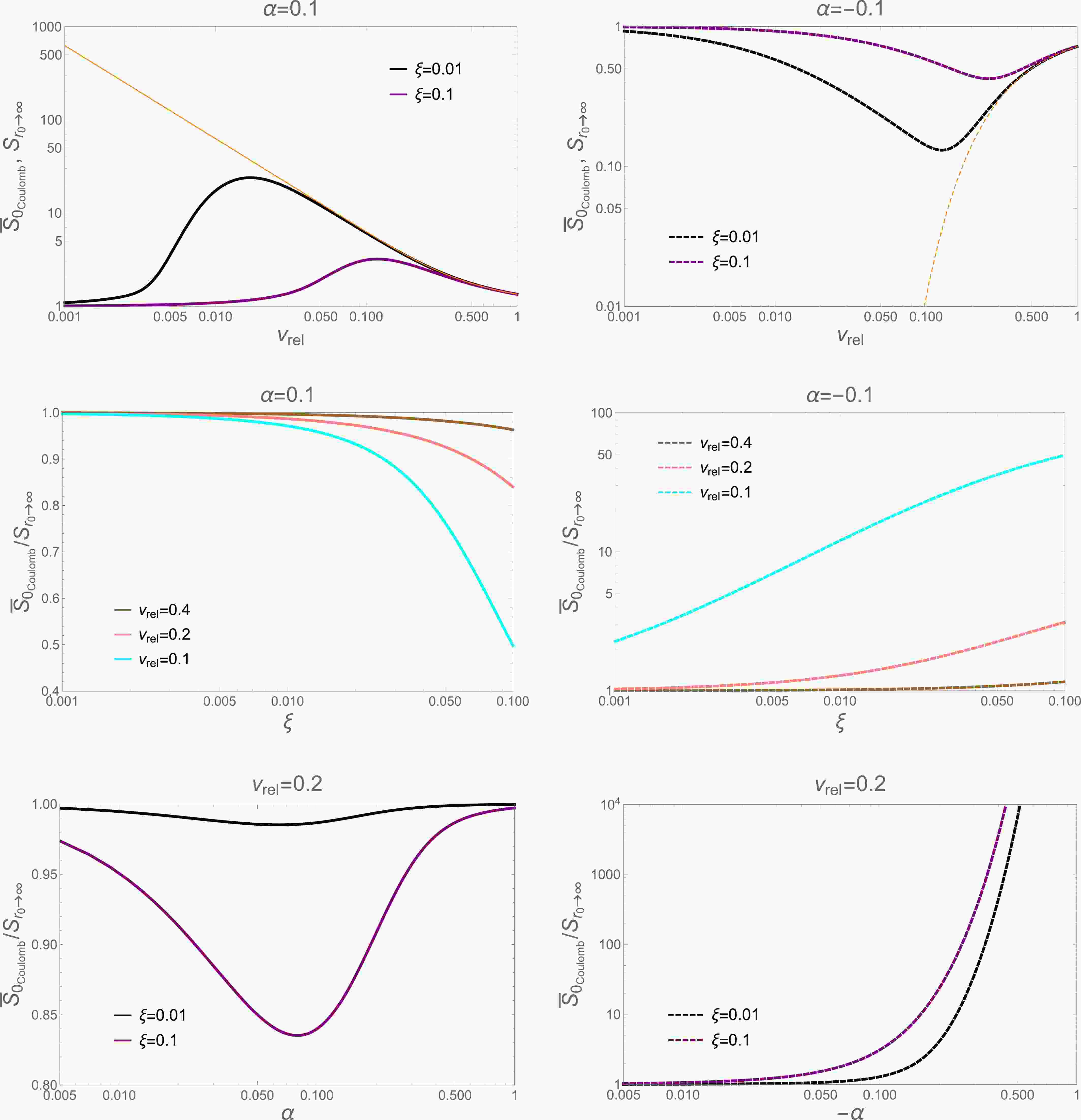
By introducing variables $\kappa \equiv \Gamma r_0/v_{\rm rel}$ and $ \xi \equiv 2 \Gamma/\mu $, the $ \eta_0 $ in $S_{0_{\rm Coulomb}}$ can be written as $\eta_0 = 2 \kappa \alpha v_{\rm rel} / \xi$. Then, $\overline{S}_{0_{\rm Coulomb}}$ becomes a function of $\xi, v_{\rm rel}/\alpha$, and $\alpha v_{\rm rel}$. Anticipating that in the next section we will average over $v_{\rm rel}$ to get the thermally averaged Sommerfeld factor, Fig. 1 shows $\overline{S}_{0_{\rm Coulomb}}$ and $\overline{S}_{0_{\rm Coulomb}}/S_{r_0 \to \infty}$ as functions of $v_{\rm rel}$, α, and ξ.

Figure 1.  (color online) Upper panels: the black and purple lines show $\bar{S}_{0_{\rm Coulomb}}$ as a function of $v_{\rm rel}$ for $\xi = 0.01$ and $0.1$, respectively. For comparison, $S_{r_0 \to \infty}$ is plotted as an orange line. Middle panels: ratio of $\bar{S}_{0_{\rm Coulomb}}$ to $S_{r_0 \to \infty}$ as a function of ξ. The brown, pink, and cyan lines represent $v_{\rm rel} = 0.4$, $0.2$, and $0.1$, respectively. In both the upper and middle panels $|\alpha| = 0.1$ is used. Lower panels: ratio of $\bar{S}_{0_{\rm Coulomb}}$ to $S_{r_0 \to \infty}$ as a function of α for $v_{\rm rel} = 0.2$. Again, the black and purple lines are for $\xi = 0.01$ and $0.1$, respectively. All left panels are for attractive Coulomb potentials where $\alpha > 0$, while all right panels are for repulsive ones where $\alpha < 0$.

The left and right panels are for attractive and repulsive Coulomb potentials, respectively. In the upper panels, we choose $ |\alpha| = 0.1 $. The black and purple lines are for $\overline{S}_{0_{\rm Coulomb}}$ with $ \xi = 0.01 $ and 0.1, respectively. The orange line is for $ S_{r_0 \to \infty} $ with the same α. The lines merge at large $v_{\rm rel}$. In the limit $v_{\rm rel} \to \infty$, both $\overline{S}_{0_{\rm Coulomb}}$ and $ S_{r_0 \to \infty} $ go to 1. In the other limit $ v_{\rm rel} \to 0 $, $\overline{S}_{0_{\rm Coulomb}}$ goes to 1, while $ S_{r_0 \to \infty} $ diverges for an attractive Coulomb potential and exponentially vanishes for a repulsive one. Between these two limits, with an increase in$v_{\rm rel}$, $\overline{S}_{0_{\rm Coulomb}}$ first increases (decreases) and then decreases (increases) for an attractive (repulsive) potential. On the contrary, $ S_{r_0 \to \infty} $ changes monotonically. These behaviors can be understood intuitively. Without considering decays, when two particles in a pair approach each other with a slow relative velocity, they feel the Coulomb force for a long period of time before they meet and annihilate; thus, the change of their wave function is large, and the Sommerfeld enhancement or suppression is significant. However, the picture is different when particle decay is taken into account. For a small $v_{\rm rel}$, the initial separation of the two particles in a pair must be small; otherwise, a decay is likely to occur before the two particles meet. If $v_{\rm rel}$ is very small, the dominant contribution to $\overline{S}_{0_{\rm Coulomb}}$ comes from pairs with small $ |\eta_0| $, and we see from Eq. (5) that $S_{0_{\rm Coulomb}} \to 1$ as $ |\eta_0| \to 0 $. For a large $v_{\rm rel}$, the two particles in a pair have a good chance to meet before a decay occurs, even if their initial separation is not small. We can see that, in general, decay makes Sommerfeld factors less prominent compared to situations when the annihilating particles are stable. That is, when annihilating particle decays need to be considered, for a given set of α and $v_{\rm rel}$, the enhancement factor is not so large for an attractive Coulomb potential, and the suppression factor is not that small for a repulsive one. The larger the decay rate, the less prominent the Sommerfeld factor. As we discussed in the Introduction, the Sommerfeld effect becomes ineffective when $\sim (\mu v_{\rm rel})^{-1}$ is larger than $\sim v_{\rm rel}/\Gamma$. This qualitatively explains why the purple lines deviate from the orange lines in the upper panels at a larger $v_{\rm rel}$, compared to the black lines.

Before we discuss other panels of Fig. 1, we first estimate the value of ξ for a coannihilator pair. For simplicity, consider that the coannihilator is a complex scalar $ \tilde{C} $ with mass m, and it decays into a Majorana DM χ with mass $ m_{\rm{DM}} $ and Dirac fermion f with a negligible mass compared to $ \Delta m \equiv m - m_{\rm{DM}} $. From the Lagrangian $\mathcal{L} = c_d \tilde{C} \overline{\chi} f +\rm h.c.$, where $ c_d $ is a dimensionless coupling, one can obtain the decay rate $\Gamma_{\tilde{C}} = 2 \dfrac{|c_d|^2}{4\pi} \dfrac{(\Delta m)^2}{m} \left(1- \dfrac{\Delta m}{2 m}\right)^2$. Therefore, $\xi = 8 \Gamma_{\tilde C}/m = 16 \dfrac{|c_d|^2}{4\pi} (\Delta m / m)^2 \left(1- \dfrac{\Delta m}{2 m}\right)^2$. Up to the factor $ \dfrac{|c_d|^2}{4\pi} $, ξ is 0.0016, 0.014, 0.14, and 0.52 for $ \Delta m / m = 0.01 $, 0.03, 0.1, and 0.2, respectively. For a larger $ \Delta m / m $, ξ is larger, but usually, the coannihilation mechanism is ineffective. We consider $ \dfrac{|c_d|^2}{4\pi} < 1 $ for a perturbative coupling, and therefore, we plot the range of ξ from $ 0.001 $ to $ 0.1 $ in the middle panels, and we show cases of $ \xi = 0.01 $ and 0.1 in the upper and lower panels, respectively.

Referring back to Fig. 1, the middle panels show $\overline{S}_{0_{\rm Coulomb}}/S_{r_0 \to \infty}$ as a function of ξ for $ |\alpha| = 0.1 $ and three choices of $v_{\rm rel}$, 0.4, 0.2, and 0.1. In sequence, these values of $v_{\rm rel}$ are typical for annihilating pairs during freeze-out when the temperature T decreases from $ \sim m_{\rm{DM}} / 25 $ to $ \sim m_{\rm{DM}} / 100 $ and to $ \sim m_{\rm{DM}} / 400 $. However, we should also keep in mind that $v_{\rm rel}$ has a Maxwell-Boltzmann distribution for a given temperature. Therefore, for example, there are some pairs with $v_{\rm rel} \sim 0.1$ or even smaller at $ T \sim m_{\rm{DM}} / 25 $. For each $v_{\rm rel}$, $\overline{S}_{0_{\rm Coulomb}}/S_{r_0 \to \infty}$ monotonically decreases (increases) from 1 with increasing ξ for an attractive (repulsive) potential. For a given ξ, the change is larger for smaller $v_{\rm rel}$. That is, the modification of the Sommerfeld factor due to decays of annihilating particles is more prominent for larger ξ and/or smaller $ v_{\rm rel} $.

The lower panels show $\overline{S}_{0_{\rm Coulomb}}/S_{r_0 \to \infty}$ as a function of $ |\alpha| $ for $ v_{\rm rel} = 0.2 $. The black and purple lines are for $ \xi = 0.01 $ and $ \xi = 0.1 $, respectively. In the limit $ |\alpha| \to 0 $, both $\overline{S}_{0_{\rm Coulomb}}$ and $ S_{r_0 \to \infty} $ go to 1. For attractive cases, $\overline{S}_{0_{\rm Coulomb}}/S_{r_0 \to \infty}$ is close to 1 at large α for the choices of $v_{\rm rel}$ and ξ, and it deviates from 1 the most at around $ \alpha \sim 0.1 $. For repulsive cases, the deviation increases with increasing $ |\alpha| $. For both attractive and repulsive potentials, the deviations are greater for larger ξ, as a larger decay rate makes the Sommerfeld enhancement or suppression less effective.

We are now in a position to consider coannihilators' decay effect on their Sommerfeld factor and consequently on the DM thermal relic abundance. In this work, we consider the simplest coannihilation scenario, where there is only one species of DM particle χ and one species of coannihilator $ \tilde{C} $. We assume that during freeze-out, the interconversion rate between χ and $ \tilde{C} $ is large enough in comparison to the Hubble expansion rate so that for a given temperature, the ratio of their number densities $ \dfrac{n_\chi}{n_{\tilde{C}}} $ equals the equilibrium value $ \dfrac{n^{eq}_\chi}{n^{eq}_{\tilde{C}}} $. This assumption is justified by our setup, where we study cases in which the decay rate of $ \tilde{C} $ into χ is much larger than the Hubble expansion rate. Therefore, the DM thermal relic abundance can be obtained by solving a single Boltzmann equation:

where x is defined as the ratio of DM mass $ m_{\rm{DM}} $ to temperature T, i.e., $ x \equiv m_{\rm{DM}} / T $. The entropy density is

$ H(m_{\rm{DM}}) $ is related to the Hubble expansion rate $ H(T) $ as follows:

where the Planck mass is $ m_{\rm{pl}} \approx 1.22 \times 10^{19} $ GeV. $ g_{\ast s} $ and $ g_\ast $ are the total numbers of effectively massless degrees of freedom associated with the entropy density and energy density of the thermal bath, respectively. We assume that χ and $ \tilde{C} $ have the same temperature as the Standard Model thermal bath. This can be achieved if interaction rates between dark sector particles and Standard Model sector particles are large enough in comparison to the Hubble expansion rate. Because we are not committed to a specific dark sector model and the possibility that the two sectors have different temperatures is not important to the physics we want to focus on in this work, we take the simplest assumption. The yield Y and its equilibrium value $ Y_{eq} $ are defined as $ Y \equiv \dfrac{n_\chi + n_{\tilde{C}}}{s} $ and $Y_{eq} \equiv ({n_\chi^{eq} + n_{\tilde{C}}^{eq}})/{s}$, respectively. To maximize the coannihilators' Sommerfeld effect on DM thermal relic abundance, in our calculation, we neglect the (co)annihilation cross sections of $ \chi \chi $ and $ \chi \tilde{C} $. Therefore, the thermally averaged effective annihilation cross section (times relative velocity) is

where $ \Delta m $ is the mass difference between the coannihilator and DM, i.e., $ \Delta m \equiv m - m_{\rm{DM}} $. $ g_{\rm{eff}} $ is given as

where $ g_\chi $ and $ g_{\tilde{C}} $ are the degrees of freedom of the DM particle and coannihilator, respectively. $ \sigma_{\tilde{C} \tilde{C}} $ is the usual spin-averaged (and also averaged over other intrinsic degrees of freedom, e.g., color, if applicable) cross section. If χ is not its own antiparticle, $ g_\chi $ includes the contributions of both χ and $ \overline{\chi} $. The same applies to $ g_{\tilde{C}} $ as well, but the $ \sigma_{\tilde{C} \tilde{C}} $ in Eq. (10) should then be replaced by $ (\sigma_{\tilde{C} \tilde{C}} + \sigma_{\tilde{C} \overline{\tilde{C}}})/2 $. A detailed explanation of the factor of $ 2 $ can be found in the Appendix of [31]. We assume that the number densities of particles and antiparticles are the same. We will consider that either $\langle\sigma_{\tilde{C} \overline{\tilde{C}}} v_{\rm rel} \rangle$ or $\langle\sigma_{\tilde{C} \tilde{C}} v_{\rm rel} \rangle$ dominates, and the Sommerfeld effect can be either an enhancement or suppression. This means applying Eq. (10) to either the attractive or repulsive case, no matter whether $ \tilde{C} $ is its own antiparticle.

By integrating Eq. (7) from a small x when $ Y = Y_{eq} $ to its value today, which essentially corresponds to $ x \to \infty $, we get today's yield, denoted by $ Y_0 $. The DM relic abundance $ \Omega h^2 $ is related to $ Y_0 $ as follows [32]:

We consider s-wave annihilations. For a Coulomb potential,

where $ a_{\tilde{C} \tilde{C}} $ is a constant, which is the s-wave value of $ \sigma_{\tilde{C} \tilde{C}} v_{\rm rel} $ without considering the Sommerfeld factor. $ \langle \overline{S}_{0_{Coulomb}}\rangle $ is the thermally averaged Sommerfeld factor, given as

where $\overline{S}_{0_{\rm Coulomb}}$ is given in Eq. (6), and it is a function of α, ξ, and $v_{\rm rel}$. Therefore, $\langle \overline{S}_{0_{\rm Coulomb}}\rangle$ is a function of α, ξ, and $ m/T $.

In Fig. 2, we plot $\langle \overline{S}_{0_{\rm Coulomb}}\rangle$ as a function of $ m/T $, using solid and dashed lines. The black and purple colors are for $ \xi = 0.01 $ and $ 0.1 $, respectively. Because the lower-left panel of Fig. 1 shows that the modification of coannihilators' Sommerfeld factor reaches its maximum at around $ \alpha \sim 0.1 $for an attractive Coulomb potential, we choose $ \alpha = 0.1 $ in the left panel of Fig. 2. For comparison, for the repulsive case, we show $ \alpha = - 0.1 $ in the right panel, although we recall that the modification of coannihilators' Sommerfeld factor increases with increasing $ |\alpha| $, as can be seen in the lower-right panel of Fig. 1. The solid and dashed orange lines show $ \langle S_{r_0 \to \infty}\rangle $, which is the thermally averaged s-wave Sommerfeld factor without considering decays of coannihilators, that is,

Figure 2.  (color online) Thermally averaged s-wave Sommerfeld factors, $\langle \bar{S}_{0_{\rm Coulomb}}\rangle$ (solid and dashed lines), $\langle S_{\rm cut}\rangle$ (dotted lines), and $\langle S_{\rm Green} \rangle$ (dot-dashed lines) for a Coulomb potential for a pair of unstable annihilating particles, as functions of the ratio of annihilating particle's mass to temperature. The black and purple lines are for $\xi = 0.01$ and $0.1$, respectively. For comparison, we use orange lines to plot $\langle S_{r_0 \to \infty}\rangle$, which is the thermally averaged s-wave Sommerfeld factor without considering decays of annihilating particles. The left panel is for an attractive potential, where $\alpha = 0.1$, while the right panel is for a repulsive one where $\alpha = - 0.1$.

The orange line monotonically increases (decreases) with increasing $ m/T $ for the attractive (repulsive) case, as the typical $v_{\rm rel}$ is smaller for larger $ m/T $. The black and purple lines are closer to 1 compared to the orange lines. One can see that when decays of coannihilators are considered, both the Sommerfeld enhancement and suppression are weaker. The modification of the thermally averaged Sommerfeld factor is more significant for larger ξ. Contrary to the monotonic behavior of the orange lines, the solid (dashed) black and purple lines first increase (decrease) with increasing $ m/T $ and then go to 1 when $ m/T $ is sufficiently large. This behavior was explained when we were discussing the upper panels of Fig. 1. For the attractive case, the difference between the solid black (purple) line and orange line at $ m/T = 25 $ is approximately 1% ($ 11 $%), while it becomes $ 4 $% ($ 45 $%) at $ m/T = 200 $. For the repulsive case, the dashed black (purple) line is higher than the orange line by approximately $ 3 $% ($ 24 $%) at $ m/T = 25 $ and by a factor of approximately 0.9 (4.5) at $ m/T = 200 $.

Before we compute the DM thermal relic abundance, we first compare the thermally averaged Sommerfeld factor obtained in this work with those calculated by two other methods.

The first method is the velocity-cut method used in our previous work [23]. In this method, by using the notation in the current work, the thermally averaged s-wave Sommerfeld factor taking into account coannihilators' decay is given as

where $H (v_{\rm rel} - v_{\rm cut})$ is the Heaviside step function, and the cut-off velocity $v_{\rm cut}$ is equal to $ \sqrt{\xi/2} $. We plot $\langle S_{\rm cut}\rangle$ using dotted lines in Fig. 2. By comparing the dotted lines with the solid or dashed lines of the same color, we can see that the general behaviors of the curves are the same. Also, curves with the same color are close at small $ m/T $, while the velocity-cut method gives a larger effect at large $ m/T $. This indicates that the results in the current work are more conservative.

The second method is the Green's function approach based on non-relativistic quantum field theory. The s-wave Sommerfeld factor, adapted to our notation, can be written as (see Eq. (4.8) of [33])

The free Green's function is given by

The Coulomb Green's function is [34]

where the ν appearing in the argument of the Gamma function $\Gamma (1- \mathrm{i} \nu)$ is $\nu \equiv \dfrac{\alpha \mu}{\sqrt{2 \mu \left(\dfrac{1}{2} \mu v_{\rm rel}^2 + \mathrm{i} \dfrac{\Gamma}{2}\right)}} = \dfrac{\alpha}{\sqrt{v_{\rm rel}^2 + \mathrm{i} \dfrac{\xi}{2}}}$, and $W_{\mathrm{i} \nu , \frac{1}{2}} \left(- 2 \mathrm{i} \mu r \sqrt{v_{\rm rel}^2 + \mathrm{i} \dfrac{\xi}{2}}\,\right)$ is the Whittaker function. It can be checked that when $ \xi = 0 $, $S_{\rm Green} = S_{r_0 \to \infty}$. In Fig. 2, we plot the thermally averaged $S_{\rm Green}$using dot-dashed lines:

We can see that the general behaviors of the dot-dashed lines are also similar to the corresponding solid or dashed lines of the same color. In particular, for the range of relatively smaller $ m/T $, where it is most relevant for the calculation of the DM thermal relic abundance in the coannihilation scenarios we are considering, the dot-dashed lines and corresponding solid or dashed lines are very close.

These comparisons strengthen the viability of the current method and can serve to verify our main finding that the coannihilators' decay makes the Sommerfeld enhancement or suppression less effective.

The relative change of the DM thermal relic abundance due to the modification of the Sommerfeld factor is denoted by $ \Delta \Omega/\Omega_{r_0 \to \infty} $, which is defined as

where $ (\Omega h^2)_{r_0 \to \infty} $ is $ \Omega h^2 $ but with $\langle \overline{S}_{0_{\rm Coulomb}}\rangle$ substituted by $ \langle S_{r_0 \to \infty}\rangle $ in Eq. (13).

Due to the exponential factor in Eq. (10), the coannihilation mechanism becomes ineffective for large x if $ \Delta m/m $ is relatively larger. Meanwhile, the modification of the Sommerfeld factor is negligible if $ \Delta m/m $ is too small, because a small $ \Delta m/m $ cannot give a sizable ξ. Therefore, to study $ \Delta \Omega/\Omega_{r_0 \to \infty} $ in the simple coannihilation scenario, in Fig. 3, we consider $ \Delta m/m $ between 0.03 and 0.2 for $ \xi = 0.01 $ and $ \Delta m/m $ between 0.1 and 0.2 for $ \xi = 0.1 $. These ranges of $ \Delta m/m $ and the corresponding ξ also ensure that the coupling between $ \tilde{C} $ and χ is perturbative for the simple model we discussed in Section 3. Considering that $ x = (1-\Delta m/m) (m/T) $ and because $ \Omega h^2 $ is approximately inversely proportional to $ \langle\sigma v \rangle_{\rm{eff}} $, we can estimate from Fig. 2 that $ |\Delta \Omega/\Omega_{r_0 \to \infty}| $ should be of order $ {\cal{O}} $(1%) for $ \xi = 0.01 $ and $ {\cal{O}} $(10%) for $ \xi = 0.1 $.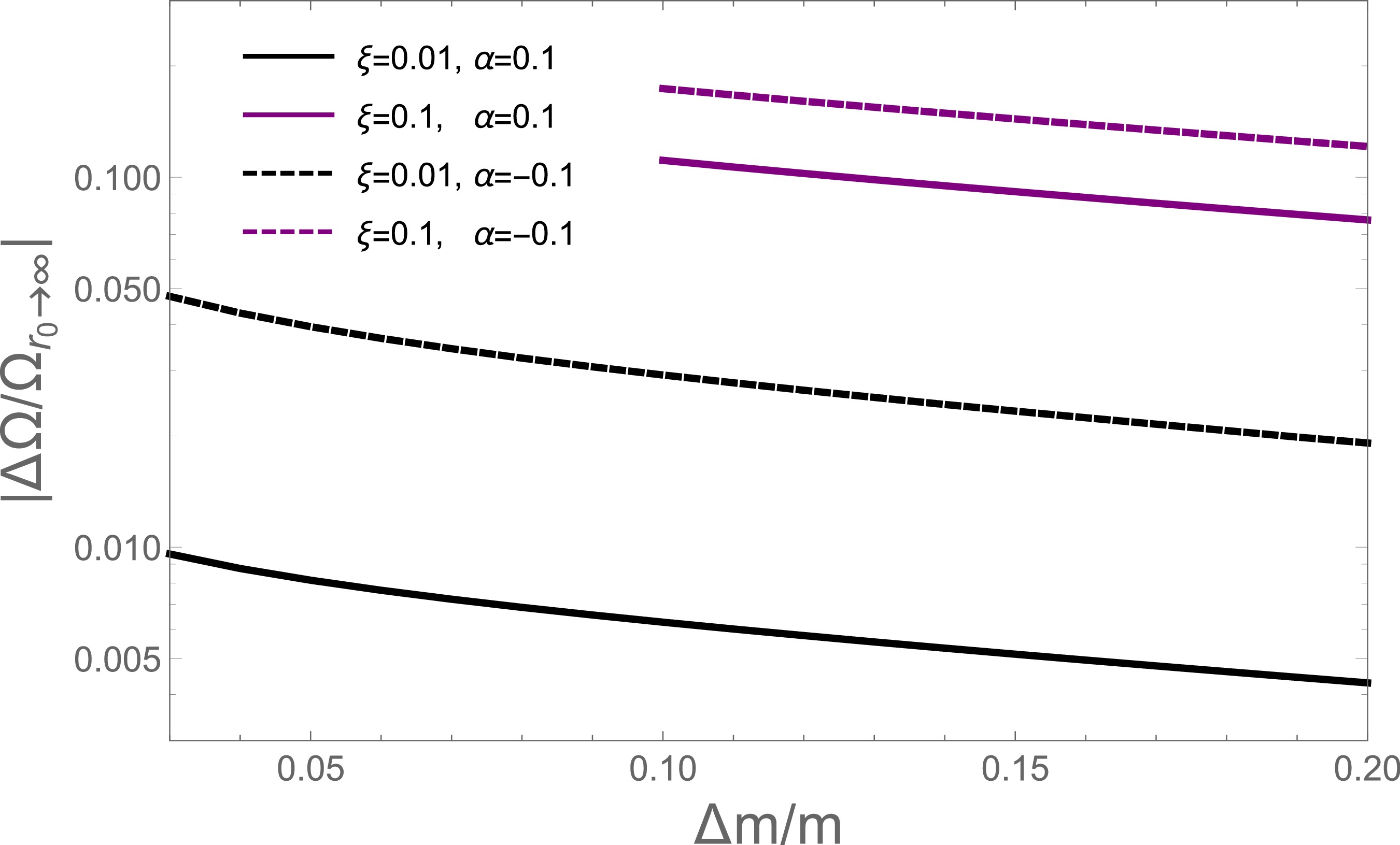

Figure 3.  (color online) Relative change of the DM thermal relic abundance due to the modification of the Sommerfeld factor induced by coannihilator decay, $\Delta \Omega/\Omega_{r_0 \to \infty}$, as a function of $\Delta m/m$. $\Delta \Omega/\Omega_{r_0 \to \infty}$ is positive for an attractive Coulomb potential, while it is negative for a repulsive one. The black and purple lines are for $\xi = 0.01$ and $0.1$, respectively. The solid lines are for an attractive potential with $\alpha = 0.1$, while the dashed lines are for a repulsive one with $\alpha = - 0.1$.

In Fig. 3, for $ \alpha = \pm 0.1 $ and $ \xi = 0.01 $ or $ 0.1 $, we plot $ |\Delta \Omega/\Omega_{r_0 \to \infty}| $ as a function of $ \Delta m/m $ for a choice of parameters $ g_\chi = g_{\tilde{C}} = 2 $, $ m_{\rm{DM}} = 2 \times 10^3 \,\text{GeV} $ and $ a_{\tilde{C} \tilde{C}} = 10^{-8} \, \text{GeV}^{-2} $. $ \Delta \Omega/\Omega_{r_0 \to \infty} $ is positive for $ \alpha = 0.1 $, while it is negative for $ \alpha = - 0.1 $. $ |\Delta \Omega/\Omega_{r_0 \to \infty}| $ decreases with increasing $ \Delta m/m $, as the coannihilation mechanism is less effective for larger $ \Delta m/m $. On each line, because ξ is fixed, the coupling between $ \tilde{C} $ and χ is smaller for larger $ \Delta m/m $. We can see that for each line, $ |\Delta \Omega/\Omega_{r_0 \to \infty}| $ is close to the difference between $\langle \overline{S}_{0_{\rm Coulomb}}\rangle$ and $ \langle S_{r_0 \to \infty}\rangle $ at $ m/T \sim 25 $ in Fig. 2, as we have estimated.

To obtain an estimate of the potential magnitude of the effect on the DM thermal relic abundance, in Fig. 4, we compute $|\langle S_{r_0 \to \infty}\rangle / \langle \overline{S}_{0_{\rm Coulomb}}\rangle - 1|$ at $ m/T = 25 $ on the ($ \alpha, \xi $) plane.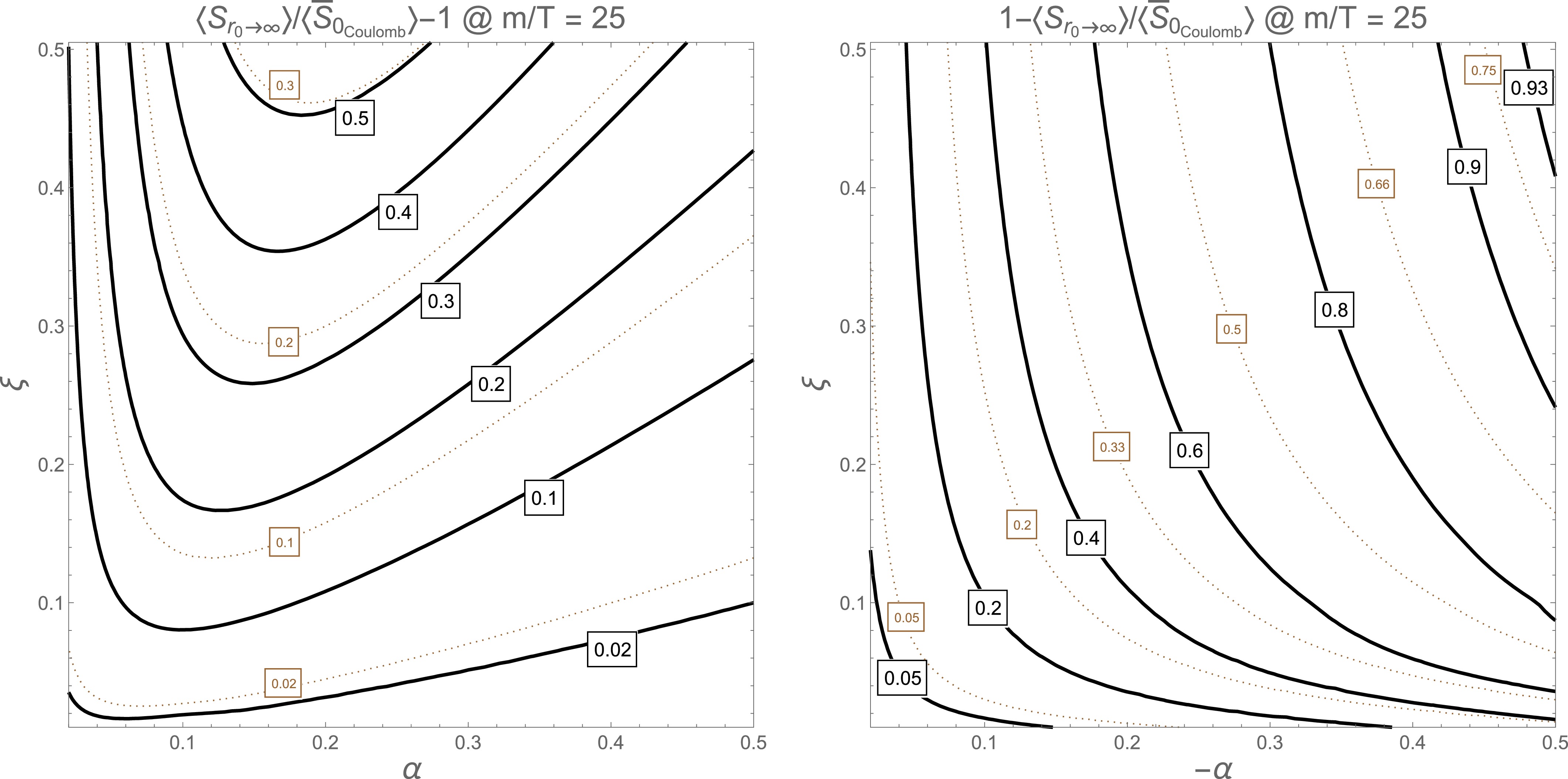

Figure 4.  (color online) The black solid lines are $|\langle S_{r_0 \to \infty}\rangle / \langle \bar{S}_{0_{\rm Coulomb}}\rangle - 1|$ contours computed at $m/T = 25$ for Coulomb potentials. The brown dotted lines are $|\Delta \Omega/\Omega_{r_0 \to \infty}|$ contours computed for $\Delta m / m = 0.2$ using $g_\chi = g_{\tilde{C}} = 2$, $m_{\rm{DM}} = 2 \times 10^3 \,\text{GeV}$, and $a_{\tilde{C} \tilde{C}} = 10^{-8} \, \text{GeV}^{-2}$. The left (right) panel is for attractive (repulsive) cases, where $\langle S_{r_0 \to \infty}\rangle / \langle \bar{S}_{0_{\rm Coulomb}}\rangle - 1$ and $\Delta \Omega/\Omega_{r_0 \to \infty}$ are positive (negative).

For both attractive and repulsive cases, for a given α, the values of contours are larger for larger ξ, meaning that a larger decay rate makes the Sommerfeld enhancement or suppression less effective. For a given ξ, for the attractive case, the values of contours first become larger and then smaller with increasing α, while for the repulsive case, the values monotonically increase with increasing $ |\alpha| $. These behaviors can also be seen in the lower panels of Fig. 1. This is due to the relative size of two length scales, namely, the initial separation of a pair of annihilating coannihilators and the Bohr radius. The modification of the Sommerfeld factor is significant when the former is comparable to or smaller than the latter. The former decreases with increasing ξ, while the latter is inversely proportional to α. For large α, while for the attractive case, $ S_{r_0 \to \infty} $ increases proportionally with increasing α, for the repulsive case, it decreases exponentially with increasing $ |\alpha| $.

For an attractive Coulomb potential, the difference between $\langle \overline{S}_{0_{\rm Coulomb}}\rangle$ and $ \langle S_{r_0 \to \infty}\rangle $ can be as much as $ \sim 50 $% for $ \alpha \sim 0.2 $ and $ \xi \sim 0.46 $. We recall that for the simple model we discussed in Section 3, to maintain a perturbative coupling between $ \tilde{C} $ and χ, $ 0.52 $ is the largest value that ξ can take for $ \Delta m / m = 0.2 $. In Fig. 4, the brown dotted lines show the $ |\Delta \Omega/\Omega_{r_0 \to \infty}| $ contours computed for $ \Delta m / m = 0.2 $ and the same choice of parameters as in Fig. 3, namely, $ g_\chi = g_{\tilde{C}} = 2 $, $ m_{\rm{DM}} = 2 \times 10^3 \,\text{GeV} $, and $a_{\tilde{C} \tilde{C}} = 10^{-8} \, \text{GeV}^{-2}$. The solid black and dotted brown contours have the same features, and they differ by less than a factor of $ 2 $. This reconfirms the viability of using $|\langle S_{r_0 \to \infty}\rangle / \langle \overline{S}_{0_{\rm Coulomb}}\rangle - 1|$ at $ m/T = 25 $ as a reasonable estimate of the effect of the modified Sommerfeld factor on the DM thermal relic abundance.

We conclude that, when there is an attractive Coulomb-like force between a pair of annihilating coannihilators, the modification of the s-wave Sommerfeld factor induced by coannihilator decay can potentially increase the calculated DM thermal relic abundance by as much as several tens of percent; when the force is repulsive, the calculated DM thermal relic abundance can be reduced by a factor of a few.

We note that the modification of the coannihilators' Sommerfeld factor is determined by α and ξ. Other quantities, such as DM mass and DM-DM in the Standard Model annihilation cross sections, determine the DM phenomenology but have little influence on the coannihilators' Sommerfeld factor. Nevertheless, because ξ is closely related to $ \Delta m $, which is a critical parameter in collider search of DM in coannihilation scenarios (for instance, jets plus missing transverse energy searches), in complete BSM models, modification of the Sommerfeld factor may lead to a shift of the parameter regions, which can both give correct DM thermal relic abundance and be testable by collider experiments.

We have calculated Sommerfeld factors for a pair of unstable annihilating particles. Due to decays, the two particles must approach each other from a finite initial separation, from where they start to feel the long-range potential generated by themselves. Consequently, conventional calculations of Sommerfeld factors, which essentially assume an infinite initial separation, may need to be modified.

To illustrate the physics, we focus our discussions on the s-wave Sommerfeld factor for a truncated Coulomb potential. We use the truncation distance to take into account the information that the initial separation of the two annihilating particles is finite. This distance is then averaged over, accounting for the probabilistic nature of decays. The resultant decay-rate-averaged Sommerfeld factors (RASFs) show that Sommerfeld effects are less prominent compared to situations when the annihilating particles are stable. The modifications are more significant for larger decay rates and/or smaller relative velocities. This confirms our intuitive idea. For an annihilation to occur, the typical initial separation of two incoming particles is given by the ratio of their relative velocity to the sum of their decay rates. Large decay rates and/or a small relative velocity lead to a small initial separation so that the accumulation of the changes of the two-body wave function from a plane wave is small, and consequently, the Sommerfeld effect is less effective.

Using the RASFs, we study thermally averaged s-wave Sommerfeld factors for a pair of unstable annihilating particles. Applying the result to a simple coannihilation scenario, we find that the modification of annihilating coannihilators' Sommerfeld factors caused by coannihilator decays may lead to a change of the DM thermal relic abundance well beyond the percent level.

Before we close, we note that there are other approaches to compute the Sommerfeld factor for unstable particles [24, 33, 35], in addition to the method based on the scattering wave function in the non-relativistic quantum mechanics framework, which we used in this work. It would be interesting to develop these approaches in the context of coannihilation scenarios, where the unstable coannihilator is customarily taken to be on-shell. This is different in collider situations, where the unstable final state particles are usually taken to be off-shell in the calculations of their Sommerfeld factors. Finally, in the parameter region where the coannihilator and DM are very degenerate in mass, the coannihilator (into DM) scattering rate, rather than the coannihilator (into DM) decay rate, dominates the coannihilator-DM interconversion rate. The investigations of this scenario will be left for future work.

The author thanks Xiaoyi Cui, Yuangang Deng, Michihisa Takeuchi, and Zhenhua Yu for helpful discussions.

Techniques for calculating the Sommerfeld factor are available in the literature (see, e.g., [8, 29, 30, 36]). In this appendix, we present a pedagogical approach for obtaining the l-wave Sommerfeld factor for a generic finite-range central-force potential $ V(r) $, meaning that $ V(r) $ vanishes for $ r > r_0 $. We require that the potential satisfies $ r^2 V(r) \to 0 $ for $ r \to 0 $. This includes the widely used Coulomb, Yukawa, and Hulthén potentials. After deriving general formulae, we give explicit expressions for a finite-range Coulomb potential, which we use in the main text.

Suppose that the long-range interaction between two massive annihilating particles can be described by a finite-range central-force potential $ V(r) $ and that the annihilation happens at $ r = 0 $, the Sommerfeld factor can be determined by solving for the scattering wave function of the Schrödinger equation for the relative motion

where we have set $ \hbar \equiv 1 $. μ is the reduced mass of the two-particle system. E is related to the relative momentum $ \boldsymbol{k} $ and the relative velocity $ v_{\rm rel} $ of the two incoming particles at large separation when $ V(r) = 0 $, satisfying $ k \equiv |\boldsymbol{k}| = \sqrt{2 \mu E} = \mu v_{\rm rel} $. Because of the axial symmetry about the z-axis, which is the direction of the incoming particles at large distance, the solution $ \psi (\boldsymbol{r}) $ takes the form

where $ A_l $ are constants and $ P_l (\cos\theta) $ are the Legendre polynomials. θ is the angle between $ \boldsymbol{r} $ and the z-axis. $ R_{kl} (r) $ are the radial functions associated with the orbital angular momentum quantum number l, and these functions are real.

Working with spherical coordinates, using

and the orthogonal relation

for each l, Eq. (22) gives

One can solve for $ R_{kl} (r) $ for both the ranges of $ r < r_0 $ and $ r > r_0 $. In either range, the solution has two constants. The total four constants are determined by the following four conditions. The requirement that $ R_{kl} (r) $ is finite as $ r \to 0 $ gives one condition:

In the range $ r > r_0 $, $ V(r) = 0 $, and $ R_{kl} (r) $ takes the form

where $ j_l (kr) $ and $ y_l (kr) $ are spherical Bessel functions of the first and second kind, respectively. $ c_{l_{\rm{outer1}}} $ and $ c_{l_{\rm{outer2}}} $ are real constants. The asymptotic form of $ R_{kl} (r) $ at $ r \to \infty $ is

One can choose to normalize $ R_{kl} (r) $ such that

where $ \delta_l $ is the phase shift, which is real. The normalization gives the relations $ c_{l_{\rm{outer1}}} = 2k \cos\delta_l $ and $ c_{l_{\rm{outer2}}} = - 2k \sin\delta_l $, such that Eq. (29) becomes

This is the second condition. The third and fourth conditions are that $ R_{kl} (r) $ and $\dfrac{\mathrm{d} R_{kl} (r)}{\mathrm{d}r}$ are continuous at $ r = r_0 $.

The l-wave Sommerfeld factor is

where $\psi_{l,\rm free} (r)$ is the l-wave function without the potential term for all r in Eq. (22), and it can also take the form of Eq. (23),

We can obtain$ A_l $ by the standard method in scattering theory (see, e.g., [37]). Making use of

and Eq. (26), and comparing the coefficients of $\mathrm{e}^{\mathrm{i}kr}$ and $\mathrm{e}^{-\mathrm{i}kr}$ of the two asymptotic forms of $ \psi (r) $,

and

we get

The scattering amplitude $ f(\theta) $ can be also obtained simultaneously, but it is not needed in deriving the Sommerfeld factor.

Without the potential term in Eq. (22) for all r, we get

where we have used the same normalization at $ r \to \infty $ and the requirement that $R_{kl,\rm free} (r) \propto r^l$ as $ r \to 0 $.

Following the same procedure as for obtaining $ A_l $, one can obtain

This is as expected, as there is no phase shift without a potential for all r. Indeed, Eqs. (34), (40), and (41) give

From Eq. (40), we have

Therefore, Eq. (33) becomes

where in the last step, we have again used the requirement that $ R_{kl} (r) \propto r^l $ as $ r \to 0 $.

In the remainder of this appendix, as an example, we derive Sommerfeld factors for a finite-range Coulomb potential, namely,

where $ \alpha > 0 $ for an attractive case and $ \alpha < 0 $ for a repulsive case.

For $ r < r_0 $, $ R_{kl} (r) $ can be written as a linear combination of the Whittaker functions

where $ \epsilon_v \equiv \dfrac{v_{\rm rel}}{\alpha} $. The condition of Eq. (28) requires that $ c_{l_{\text{inner2}}} = 0 $, so that

Using Eq. (32) and the continuity of $ R_{kl} (r) $ and $\dfrac{\mathrm{d} R_{kl} (r)}{\mathrm{e}r}$ at $ r = r_0 $, one can solve for $ c_{l_{\text{inner 1}}} $ and $ \delta_l $. Using

from Eq. (44), we get the l-wave Sommerfeld factor

For a general l, using the analytical expression of $ |c_{l_{\text{inner 1}}}|^2 $, we have checked that

which is the result given in the literature for a Coulomb potential without truncation [29, 30]. We have also checked that, as expected,

The s-wave Sommerfeld factor is

where $ \eta_0 \equiv \alpha \mu r_0 $, $ f_1 \equiv F \left(\dfrac{i}{\epsilon_v},2,2 i \epsilon_v \eta_0\right) $, and $ f_2 \equiv F \bigg(1 + \dfrac{i}{\epsilon_v},\bigg. \bigg.2,2 i \epsilon_v \eta_0\bigg) $. F is the confluent hypergeometric function given by $ F(a, b, z) = 1 + \dfrac{a}{b} \dfrac{z}{1!} + \dfrac{a(a+1)}{b(b+1)} \dfrac{z}{2!} + \cdots $.

Exchanges of some light but massive mediator between a pair of annihilating particles can give rise to a Yukawa-like potential. The main difference between Sommerfeld factors for a Coulomb and Yukawa potential is that the latter feature resonances. The importance of these resonances in DM indirect searches and relic abundance calculations has been well-studied. While the key physics that we want to convey has been illustrated in the main text by studying a Coulomb potential, we would like to investigate whether the resonance feature in Sommerfeld factors can bring more interesting results.

The procedure to obtain Sommerfeld factors outlined in Appendix A can be applied to Yukawa potentials. However, the exact Sommerfeld factor for a Yukawa potential must be obtained numerically. Fortunately, it is known that a Yukawa potential can be approximated by a Hulthén potential, for which an analytic Sommerfeld factor can be found [30]. Therefore, in this appendix, we present results for a finite-range Hulthén potential,

where $ \alpha > 0 $ for an attractive case and $ \alpha < 0 $ for a repulsive case. It was found [30] and confirmed [21] that by relating $ m_\phi^* $ with the mediator mass $ m_\phi $ as $ m_\phi^* = \dfrac{\pi^2 m_\phi}{6} $, the s-wave Sommerfeld factor for a Hulthén potential is an excellent approximation of that for a Yukawa potential $ - \alpha \mathrm{e}^{-m_\phi r}/r $.

Using the procedure described in Appendix A, we derive the analytic (though lengthy) s-wave Sommerfeld factor for this potential, $S_{0_{\rm Hulthen}}$, which is the analogue of Eq. (52) for the finite-range Coulomb potential. We have checked that, as expected,

Also,

where $ y \equiv m_\phi^*/(\mu \alpha) $, and this expression is the same as that given in the literature for a Hulthén potential without truncation ⁶.

Substituting $S_{0_{\rm Coulomb}}$ with $S_{0_{\rm Hulthen}}$ in Eq. (6), we obtain the s-wave rate-averaged Sommerfeld factor $\overline{S}_{0_{\rm Hulthen}}$, which is to be compared with $S_{r_0 \to \infty_{\rm Hulthen}}$. By further substituting $\overline{S}_{0_{\rm Coulomb}}$ with $\overline{S}_{0_{\rm Hulthen}}$ in Eq. (14) and $ S_{r_0 \to \infty} $ with $S_{r_0 \to \infty_{\rm Hulthen}}$ in Eq. (15), we obtain the thermally averaged Sommerfeld factors $\langle \overline{S}_{0_{\rm Hulthen}}\rangle$ and $\langle S_{r_0 \to \infty_{\rm Hulthen}} \rangle$, respectively, for the Hulthén potential.

For a massive mediator, researchers are usually interested in the Sommerfeld enhancement and in particular the resonance behavior. Thus, in the following, we show s-wave results for attractive Hulthén potentials and pay special attention to the largest resonance. To facilitate comparisons with the results of attractive Coulomb potentials shown in the main text, we use $ \alpha = 0.1 $ and the same two choices of ξ, namely, $ 0.01 $ (black curves) and $ 0.1 $ (purple curves).

In the left panel of Fig. B1, $\overline{S}_{0_{\rm Hulthen}}$ and ${S}_{r_0 \to \infty_{\rm Hulthen}} $ are plotted as functions of y for three choices of $ v_{\rm rel} $: 0.15, 0.01, and 0.003. For $S_{r_0 \to \infty_{\rm Hulthen}}$, it is known that the resonances are more prominent for smaller $ \epsilon_v $, and indeed, we can see the resonances clearly for $ v_{\rm rel} = 0.01 $ and $ 0.003 $. Similar to the attractive Coulomb case, for a given $ v_{\rm rel} $, $\overline{S}_{0_{\rm Hulthen}}$ is smaller for larger ξ. Additionally, we see that the resonances are more suppressed for larger ξ.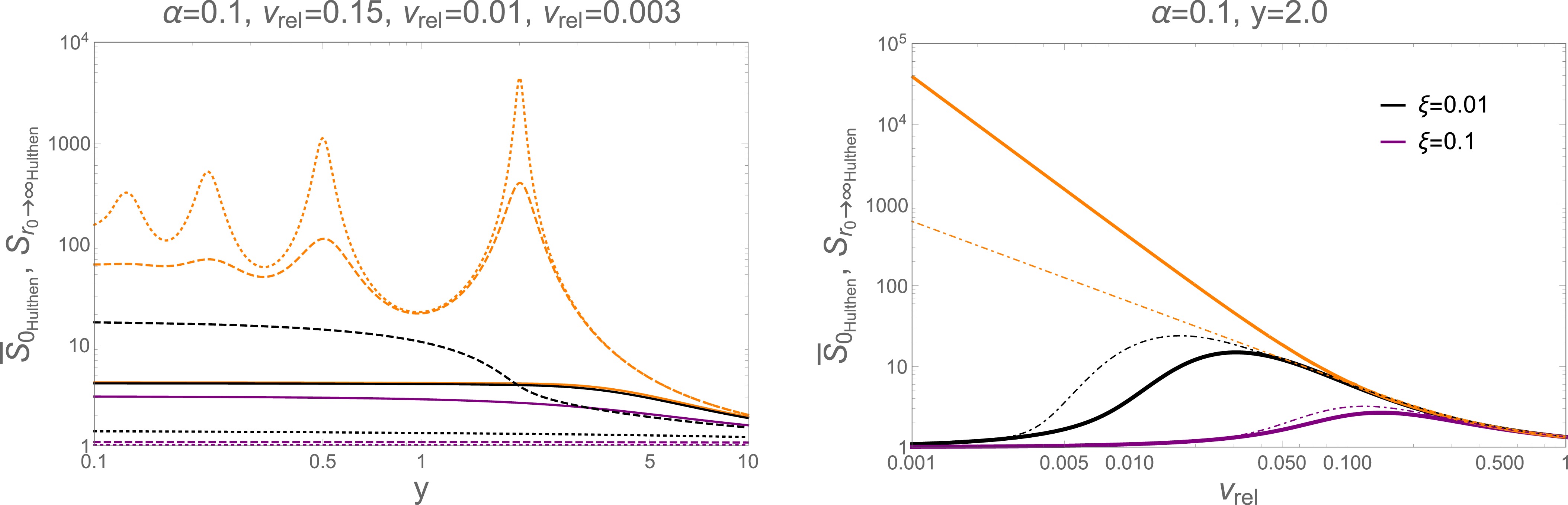

Figure B1.  (color online) In the left panel, we show $\bar{S}_{0_{\rm Hulthen}}$ (black and purple lines) and $S_{r_0 \to \infty_{\rm Hulthen}}$ (orange lines) as functions of y for three different $v_{\rm rel}$. The solid, dashed, and dotted lines are for $v_{\rm rel} = 0.15$, $0.01$, and $0.003$, respectively. In the right panel, using solid lines, we show $\bar{S}_{0_{\rm Hulthen}}$ (black and purple) and $S_{r_0 \to \infty_{\rm Hulthen}}$ (orange) as functions of $v_{\rm rel}$ for $y = 2.0$. For comparison, the curves for an attractive Coulomb potential with the same α shown in the upper-left panel of Fig. 1 are replotted here using dot-dashed lines. $\alpha = 0.1$ is used in both panels, and the black and purple lines are for $\xi = 0.01$ and $0.1$, respectively.

In the right panel of Fig. B1, $\overline{S}_{0_{\rm Hulthen}}$ and $S_{r_0 \to \infty_{\rm Hulthen}}$ are plotted as functions of $ v_{\rm rel} $ for $ y = 2.0 $, which is the value close to the position of the highest peak in the left panel. The curves are similar to those in the upper-left panel of Fig. 1 for the s-wave result of an attractive Coulomb potential. To make the comparison easier, we replot the curves of the latter case using dot-dashed lines. We can see that on the small $ v_{\rm rel} $ side, without a truncation in the potentials, the Sommerfeld factor for a Hulthén potential is much larger than that for a Coulomb potential. However, when a truncation is considered, the rate-averaged Sommerfeld factors for a Hulthén potential are smaller than those for a Coulomb potential. On the large $ v_{\rm rel} $ side, the resonance in the Hulthén case is almost invisible, and the lines with the same color merge. Other features of the curves for the Hulthén potential can be explained the same as those for the Coulomb potential, and we refer the reader to the discussions around the upper-left panel of Fig. 1 for details.

In the left panel of Fig. B2, we plot $\langle \overline{S}_{0_{\rm Hulthen}}\rangle$ and $\langle S_{r_0 \to \infty_{\rm Hulthen}} \rangle$ as functions of $ m/T $. These curves are similar to the solid ones shown in the left panel of Fig. 2, which are replotted here using dot-dashed lines. The difference between the solid and dot-dashed lines of the same color can be understood from the discussions for the right panel of Fig. B1, recalling that a larger $ m/T $ corresponds to a smaller typical value of $ v_{\rm rel} $. Again, other features of the curves for the Hulthén potential can be explained the same as those for the Coulomb potential, and one can refer to the discussions on the left panel of Fig. 2.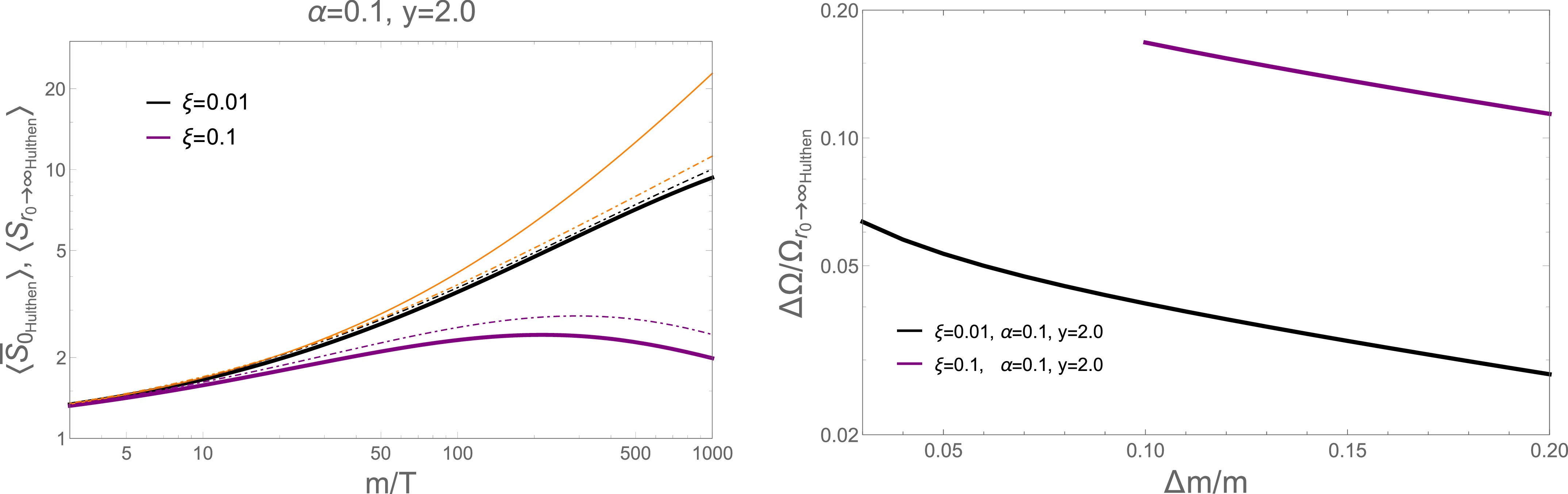

Figure B2.  (color online) Left panel: $\langle \bar{S}_{0_{\rm Hulthen}}\rangle$ (black and purple lines) and $\langle S_{r_0 \to \infty_{\rm Hulthen}} \rangle$ (orange line) for an attractive Hulthén potential for a pair of unstable annihilating particles as functions of the ratio of the annihilating particle's mass to temperature. Right panel: relative change of the DM thermal relic abundance due to modification of the Sommerfeld factor induced by coannihilator decay, $\Delta \Omega/\Omega_{r_0 \to \infty_{\rm Hulthen}}$, as a function of $\Delta m/m$ for $g_\chi = g_{\tilde{C}} = 2$, $m_{\rm{DM}} = 2 \times 10^3 \,\text{GeV}$, and $a_{\tilde{C} \tilde{C}} = 10^{-8} \, \text{GeV}^{-2}$. In both panels, $\alpha = 0.1$ and $y = 2.0$ are used, and the black and purple lines are for $\xi = 0.01$ and $0.1$, respectively. For comparison, in the left panel, the dot-dashed lines replot the curves for an attractive Coulomb potential with the same α shown by the solid lines in the left panel of Figure 2.

In the right panel of Fig. B2, we show $\Delta \Omega/\Omega_{r_0 \to \infty_{\rm Hulthen}}$ as a function of $ \Delta m/m $ for the same choice of parameters as in Fig. 3, namely, $ g_\chi = g_{\tilde{C}} = 2 $, $ m_{\rm{DM}} = 2 \times 10^3 \,\text{GeV} $, and $ a_{\tilde{C} \tilde{C}} = 10^{-8} \, \text{GeV}^{-2} $. $\Delta \Omega/\Omega_{r_0 \to \infty_{\rm Hulthen}}$ is defined the same way as in Eq. (21) but for the Hulthén potential. Compared to the corresponding solid lines in Fig. 3 for the attractive Coulomb case, it appears that the relative change of the DM thermal relic abundance is larger for the resonance in the Hulthén potential.

In this appendix, we derive Eq. (22) in Appendix A for a pair of unstable annihilating particles. The Sommerfeld factors we use in this work are determined by solving for this equation. Although this is a common starting point in the literature to derive the Sommerfeld factors, some discussions in the context when the annihilating particles can decay are needed.

The quantum mechanical approach for deriving Sommerfeld factors relies on the assumption that the distance scale for the long-range force and that for annihilation are well separated. Generally, this assumption is met because the annihilation can be approximated to occur only when the two particles collide at $ \boldsymbol{r} = 0 $. However, when annihilating particle decay is considered, one may wonder whether it is still possible to use this approach to derive Sommerfeld factors, given that the decay is now a short-distance process.

Let us start from the time-dependent Schrödinger equation for two particles, written in terms of the center-of-mass coordinate $ \boldsymbol{R} $ and relative coordinate $ \boldsymbol{r} $ as

where $ \boldsymbol{R} = \dfrac{m_1 \boldsymbol{r}_1 + m_2 \boldsymbol{r}_2}{m_1 + m_2} $, $ \boldsymbol{r} = \boldsymbol{r}_1 - \boldsymbol{r}_2 $, $ M = m_1 + m_2 $, and $ \mu = \dfrac{m_1 m_2}{m_1 + m_2} $. Γ is the sum of decay rates of the two particles. $ U(\boldsymbol{r}) $ is the sum of $ V(r) $ in Eq. (22) and the annihilation term, which is proportional to $ \delta^3(\boldsymbol{r}) $ ⁷.

As mentioned in the discussion below Eq. (6), we neglect the velocity dependence of Γ, because during and after freeze-out, the typical $ v_{\rm rel} $ is non-relativistic. Therefore, we treat Γ as a constant. Now, taking advantage of this, we can solve the above equation using a separation of variables:

where $ E_T $ is the total energy of the two-particle system. $ \psi (\boldsymbol{R}, \boldsymbol{r}) $ satisfies

and it can be further separated as $ \psi (\boldsymbol{R}, \boldsymbol{r}) = \psi_c (\boldsymbol{R}) \psi_r (\boldsymbol{r}) $, where $ \psi_c (\boldsymbol{R}) $ describes the motion of the mass center,

and $ \psi_r (\boldsymbol{r}) $ describes the relative motion of the two-particle system,

E is the relative energy appearing in Eq. (22), and the center-of-mass energy $ E_c = E_T - E $.

From Eq. (60), the usual procedure in the literature to derive Sommerfeld factors is then to neglect the annihilation term in $ U(\boldsymbol{r}) $ and solve for Eq. (22) ⁸.

Some discussion may be needed for the factor $ \mathrm{e}^{- \frac{\Gamma}{2} t} $ in Eq. (57). This factor leads to a reduction of the flux of the annihilating particle pair. However, in the context of coannihilation, the decay (and inverse-decay) of the coannihilators is traditionally taken into account in the coupled set of Boltzmann equations for the DM and coannihilators. In this sense, decay and annihilation processes of the coannihilators are in fact already simultaneously considered, no matter whether there is a Sommerfeld factor for the annihilation of coannihilators. Also, for the purpose of calculating DM relic abundance, the coupled set of Boltzmann equations can be reduced to a single Boltzmann equation if the decay rate is much larger than the Hubble expansion rate. The single Boltzmann equation is obtained by adding each of the coupled Boltzmann equations. In this way, the decay (and inverse-decay) terms cancel. Therefore, one usually does not have to consider this factor.