


 Abstract
 HTML
HTML Reference
 Related
 PDF
PDF


-
Dark matter (DM), which comprises about a quarter of the universe's mass, remains one of the most mysterious objects in particle physics. Primarily recognized through its gravitational influence on galaxies and cosmic structures, it might also be undetectable through electromagnetic means. The weakly interacting massive particle (WIMP) miracle, the suggestive coincidence of the weak coupling DM with a proper density that would have been thermally generated, motivated experimental tests through direct scattering of WIMPs, decay of WIMPs to visible cosmic rays, and DM production at collider experiments. However, no positive result has been reported thus far (for an incomplete list on this topic, please see Refs. [1−15]).
In addition to the WIMP, several other interesting DM models exist. An interesting scenario suggests that DM is likely glueballs, particles composed of strongly interacting dark gluons bound together without fermions. This scenario results from a confining dark
$S U(N)$ gauge theory extrapolated from Quantum Chromodynamics (QCD). These glueballs in the dark sector are hypothesized to interact with standard model particle primarily through gravitational forces and may contribute significantly to the DM content [16−21].Glueballs within QCD are bound states of gluons, characterized by the absence of quark constituents. These entities emerge from non-Abelian gauge theories, notably
$S U(N)$ lattice gauge theories, where non-perturbative effects support the formation of such composite particles [22−24]. This characteristic surprisingly bridges the gap between the domain of strong interactions and cosmological phenomena, suggesting a novel perspective where the dynamics of the strong force support the mysterious nature of DM. The similarities underscore the appealing hypothesis that glueballs may constitute the DM component in these scenarios [20]. Theoretical studies and simulations within this framework have been important in substantiating the glueball DM hypothesis and offering a robust statement that integrates the microcosmic interactions of particle physics with the large-scale structures and dynamics observed in the universe.Lattice QCD calculations are essential in non-perturbative studies of QCD glueballs [25−32]. This non-perturbative method offers detailed insights into key properties of glueballs, including the spectrum and decay properties. Consequently, it reveals their potential significance across a spectrum of physical phenomena. In the lattice investigation of self-interacting DM, the ratio of two-body scattering cross section to the mass of DM, denoted as
$ \sigma/m $ is of significant interest. It is not only a crucial quantity for experimental physicists seeking to constrain the characteristics of DM [33−35] but is also important in understanding cosmic phenomena, as highlighted in previous research [36]. Recent advances in lattice calculations [37, 38] have been also crucial in determining the scattering cross section of dark glueballs within the lattice$S U(2)$ Yang-Mills theory.Traditional Monte Carlo (MC) methods for lattice simulations encounter challenges such as critical slowing down [39] and topological freezing [40]. Owing to the chain-like nature of the Markov process, configurations generated by traditional methods are not strictly independent unless a very long Markov chain is achieved. Many improvements have been developed over the past decades, but another potentially promising method, inspired by machine learning (ML) concepts and techniques, is the flow-based model [41−44] (for a review, see Refs. [45, 46]). A flow-based model is a type of neural network that can learn a complicated probability distribution from data and generate new samples from it without using Markov chain MC methods. Moreover, flow-based models can also learn the potential features and correlations of the data, and provide insights into the structure and dynamics of the system. Flow-based models impose an invertible transformation constructed by neural networks transforming a simple distribution to a complex one to perform the maximum likelihood estimation.
In the remainder of this paper, we use the traditional MC method and an ML approach comparatively to generate lattice configurations for the
$S U(2)$ gauge theory with zero fermion flavors ($ N_f=0 $ ) and several coupling constants β. Subsequently, we compare the results for the dark glueball obtained from these distinct simulations. Furthermore, we calculate the interaction potential for dark glueballs and determine the interaction coupling constants in effective Lagrangian. Finally, we obtain the relation between the dark glueball mass and scattering cross section. By comparing theoretical results with experimental data, we extract the lower bound on the mass of scalar glueballs as candidates of DM. Some details are presented in the appendix. -
In this section, we exlpain the theoretical basis of our lattice simulations. This comprises the application of the
$S U(N)$ gauge theory action within both the MC method and ML approach. We elaborate on the specific ML methodology, particularly the flow-based model. Additionally, this section includes the strategy to investigate the dark glueball, demonstrating how to determine its mass, coupling constants of effective Lagrangian, and scattering cross section. -
The
$S U(N)$ gauge theory was established for describing interactions of non-Abelian gauge bosons, with$S U(3)$ gauge theory being crucial for modeling strong interactions. Explicitly, we can discretize the spacetime to simulate QCD in continuum with gauge links$ U_{\mu}(n) $ in the path integral approach [49]. Standard simulations of$S U(N)$ gauge theory utilize plaquettes$ U_{\mu\nu}(n) $ , defined as$ U_{\mu\nu}(n)=U_{\mu}(n)U_{\nu}(n+\hat{\mu})U^{\dagger}_{\mu}(n+\hat{\nu})U^{\dagger}_{\nu}(n), $

(1) where n represents the lattice coordinates, and
$ \mu,\nu $ represents gauge link directions. The discretized action is constructed as$ S[U]=\frac{\beta}{N}\sum\limits_{n,\mu<\nu}\mathrm{Re}\;\mathrm{tr}\left[1-U_{\mu\nu}(n)\right], $

(2) where β is related to the coupling constant:
$ \beta=2N/g^2 $ . N signifies the color degree of freedom within the$S U(N)$ gauge field, which is set to 2 in this study. The action described previously is referred to as the naive action.The Lüscher-Weisz (improved) action is frequently employed to reduce lattice spacing discretization effects, [50], in which both plaquettes
$ U_{\mu\nu}(n) $ and rectangles$ R_{\mu\nu}(n) $ are considered:$ \begin{aligned}[b] R_{\mu\nu}(n)= & U_{\mu}(n)U_{\mu}(n+\hat{\mu})U_{\nu}(n+2\hat{\mu})\\ & U^{\dagger}_{\mu}(n+\hat{\mu}+\hat{\nu})U^{\dagger}_{\mu}(n+\hat{\nu})U^{\dagger}_{\nu}(n). \end{aligned} $

(3) The corresponding action is constructed as
$ \begin{aligned}[b] S[U]=&\frac{\beta}{2N}\mathrm{Re}\Big[\sum\limits_{n,\mu<\nu}c_0\mathrm{tr}\left(1-U_{\mu\nu}(n)\right)\\ & +\sum\limits_{n,\mu,\nu}c_1\mathrm{tr}\left(1-R_{\mu\nu}(n)\right)\Big], \end{aligned} $

(4) where the coefficients for plaquettes and rectangles are
$ c_0=5/3 $ and$ c_1=-1/12 $ , respectively.Our study aims to apply self-interacting gauge fields to explore DM, where we opt for simplicity by setting
$ N=2 $ . We plan to employ both naive and improved actions for MC simulations, and the naive action in combination with ML simulations, as detailed in Section III. -
In the flow-based model [41−44], the process begins with a basic prior distribution
$ r(z) $ that is easy to sample. With this, a collection of samples$ {z_i} $ can be produced and subjected to a reversible one-to-one transformation$ f(z) $ . Consequently, the transformed samples$ x_i=f(z_i) $ inherently conform to a new distribution$ q(x) $ :$ q(x)=r(z)[J(z)^{-1}]=r(z)\left | {\det}\frac{\partial f(z) }{\partial z } \right |^{-1},~~ z=f^{-1}(x). $

(5) The objective is to align the new distribution
$ q(x) $ more closely with the target distribution$ p(x) $ , which takes the form$p(x)= {\rm e}^{-\beta S(x)}/Z$ under lattice gauge theory. To assess this alignment, we can make utilize the Kullback-Leibler (KL) divergence [47]. The KL divergence between two distributions$ q(x) $ and$ p(x) $ , denoted as$ D_{KL}(q|p) $ , is defined as$ D_{\text{KL}}(q | p) = \int {\rm d} x\,q(x) \log \left( \frac{q(x)}{p(x)} \right) \geq 0. $

(6) A low KL divergence suggests a close similarity between the two distributions, and
$ D_{KL}(q|p)=0 $ only when$ q(x)=p(x) $ . In this context, we can construct the transformation as a sequence of neural networks and employ the KL divergence between the resultant distribution$ q(x) $ and the target distribution$ p(x) $ as a loss function for network training. Throughout the training phase, the KL divergence can be approximated using the sample mean value:$ loss=E_q \left( \log \frac{q(x)}{p(x)}\right) \approx \frac{1}{N} \sum\limits_{i=1}^N \log \frac{q(x_i)}{p(x_i)}. $

(7) Within the flow-based model, the design of the invertible transformation
$ f(z) $ demands careful consideration because the Jacobian determinant of$ f(z) $ influences the resulting distribution$ q(x) $ . For optimized efficiency, the transformation is structured to yield an upper or lower triangular matrix for the Jacobian. More explicitly, we can first select certain components of z to transform, such as$z^1, z^2,...,z^k$ (where upper indices denote different components of the variable) and keep the remaining components$z^{k+1},z^{k+2},...,z^n$ frozen, i.e.,$f(z^{j})=z^{j},\; k+1 \leq j \leq n$ . The overall transformation, which is composed of many single transformations with different frozen freedoms, can transform the samples completely, such that every component of z is transformed at least once. Next, we can define a set of invertible one-to-one mappings$ F(z; \alpha_i) $ for$ 1 \leq l \leq k $ with the$ \alpha_i $ s being parameters. For example, if$ z^l \in \mathbb{R} $ , we can set the one-to-one maps as$F(z^l; \alpha_i)= \alpha_1 z^l + \alpha_2$ with$ \alpha_1 > 0 $ . Subsequently, we can construct neural networks that utilize the fixed components as inputs and output the parameters of the mappings, i.e., the networks map the fixed components to the parameters:$ \{\alpha_i\} = F_{NN}(z^{k+1},z^{k+2}...z^n; \omega_\lambda). $

(8) Here,
$ F_{NN} $ denotes the neural network transformation, which is typically non-invertible or difficult to invert, whereas the transformation applied to the samples remains invertible. The neural network parameters, denoted as$ \omega_\lambda $ , must be optimized. Incorporating fixed components as inputs to the neural networks enhances the overall expressiveness of the transformation and enables correlations among the various components.Under the above transformation, the Jacobian is structured as follows:
$ \mathbf{J}= \begin{bmatrix} \dfrac{\partial x^i}{\partial z^j} \delta_{ij} & \dfrac{\partial x^l}{\partial z^j} \\ \mathbf{0} & \mathbf{I}_{n-k} \end{bmatrix}, \;1 \leq i,j \leq k,\; k+1 \leq l \leq n. $

(9) This results in an upper triangular matrix whose determinant can be efficiently computed.
By following these steps, we can illustrate the implementation of the flow-based model in 4-dimensional
$S U(2)$ lattice gauge theory. For further insights, refer to [52]. The prior distribution is established as a uniform distribution with respect to the Haar measure of the$S U(2)$ group owing to its numerical sampling convenience.First, the fixed components of the gauge fields should be selected. For a 4-dimensional lattice with coordinates
$n_i,\; i=0,\,1,\,2,\,3,\; n_i \in \mathbb{Z}$ , a translational phase is defined based on a translation vector$ \mathbf{t} $ , where$ t_i \in \mathbb{Z} $ :$ \phi(n) = \sum\limits_i n_i t_i \mod 4. $

(10) This method divides the entire lattice into four segments based on their respective phase values. During a single transformation, one direction of the link variables within a segment is designated as the actively transformed component, and the others are fixed. By combining a minimum of 16 individual transformations, we achieve a comprehensive transformation. In our numerical experiments, we set the translation vector to
$ (0,1,2,1) $ and designate$ U_0(n) $ as the active transformed link direction.Second, one-to-one mappings are designed. In gauge theory, the gauge invariance of the theory must be preserved. Therefore, as link variables are not gauge covariant, they are not directly transformed. Instead, the plaquettes containing the actively transformed links are transformed. Describing the one-to-one mapping on plaquettes or in
$ S U(2) $ group space directly in numerical terms is challenging. However, by considering the theory’s requirement for gauge covariance, we can confine the mapping to$ f(XPX^{-1}) = Xf(P)X^{-1} $ , where P and X belong to$ S U(2) $ . We can prove that, given the diagonalization of P,$ P=SUS^{-1} $ the requirement is equivalent to$ f(P) = Sf(U)S^{-1},\; U = \text{diag} ({\rm e}^{{\rm i}\theta_1},{\rm e}^{{\rm i}\theta_2}). $

(11) In other words, only the eigenvalues must be transformed. The two eigenvalues are not independent of each other owing to the constraint
$ \det P=1 $ , which results in$ \theta_1+\theta_2=0 $ . We can design diagonalization procedure to make$ \theta_1 \geq 0, \theta_2 \leq 0 $ ; subsequently,$ P=S \begin{bmatrix} {\rm e}^{{\rm i}\theta} & 0 \\ 0 & {\rm e}^{-{\rm i}\theta} \end{bmatrix} S^{-1}, \quad 0 \leq \theta \leq \pi. $

(12) The one-to-one mapping can now be simplified as
$ f(P)=S \begin{bmatrix} {\rm e}^{{\rm i}f(\theta)} & 0 \\ 0 & {\rm e}^{-{\rm i}f(\theta)} \end{bmatrix} S^{-1},\quad 0 \leq f(\theta) \leq \pi. $

(13) The requirement now reduce to that
$ f(\theta) $ should be a one-to-one map on interval$ [0, \pi] $ . In our numerical simulations, we opt for the rational-quadratic neural spline flow method with five nodes as the one-to-one mapping on the interval$ [0, \pi] $ owing to its high flexibility. This choice is based on Ref. [53].In constructing the neural network, maintaining gauge covariance necessitates that inputs consist solely of plaquettes containing frozen link variables. To ensure the translation invariance and cyclic boundary conditions inherent in lattice theory, the optimal architecture involves convolutional neural networks (CNNs) with cyclic padding. In our simulations, we used a four-dimensional CNN with a kernel size of 3 and 48 hidden channels, employing LeakyReLU as the activation function and the Adam optimizer for training. A mask, shaped to match the lattice plaquettes, was applied to select the frozen plaquettes before they are inputted.
Although the flow-based model has been proven to be effective, it encounters the mode collapse problem when β increases [54]. A quenched method was proposed in Ref. [55] to solve this problem. The quenched method involves first training a model to generate samples that adhere to the distribution
${\rm e}^{-\beta_1 S(x)}/Z_1$ , where$ \beta_1 $ is small. Subsequently, this distribution with a small$ \beta_1 $ is utilized as the prior distribution to train a second model that generates samples following${\rm e}^{-\beta_2 S(x)}/Z_2$ with a larger$ \beta_2 $ . This process is iterated until the value of β reaches the desired level. In this study, we begin with$ \beta=0 $ and incrementally vary β by 0.1 or 0.2 every 10 or 20 rounds of training until β reaches the target value. Thus, the total training time is reduced compared with the original method, and an advantage is that only one model needs to be saved. The overall training time increases approximately linearly with β and the lattice volume (the number of training parameters increases approximately linearly with the lattice volume), whereas the time required for generating configurations is dependent only on the lattice volume. At this point, note that the flow-based model is inefficient in generating configurations with a very large volume. For a comparative analysis in this study, we set β up to 2.2 and the lattice volume up to$ 10^4 $ . -
In lattice simulations, the operator for dark glueball with
$ J^{PC}=0^{++} $ is given:$ \hat{O}(t,\vec{x})=\mathrm{Re} \;\;\mathrm{tr}\sum\limits_{\mu<\nu}U_{\mu\nu}(t,\vec{x}). $

(14) To account for the vacuum state sharing the quantum numbers of the glueball
$ J^{PC}=0^{++} $ , we subtract the vacuum expectation value, reformulating the operator as$\hat{O}^{\prime}(t,\vec{x})= \hat{O}(t,\vec{x})-\langle\hat{O}(t,\vec{x})\rangle$ . We can use two-point correlation functions to determine the mass of dark glueball:$ C_2(t)=\sum\limits_{\vec{x}, \vec{y}}\langle0|\hat{O}(t,\vec{x})\hat{O}(0,\vec{y})|0\rangle. $

(15) When the time slice t is sufficiently large, the two-point correlation function is reduced to
$ C_2(t) \sim C_0 {\rm e}^{-E_0t}. $

(16) The effective energy
$ E_0 $ represents the energy of the lowest dark glueball state (ground state), and when the momentum is zero, it is reduced to the mass$ m_g $ .In contrast to the naive action, the operator formulation for the dark glueball in the context of the improved action incorporates an additional rectangular term, as defined in Eq. (3). Thus, the operator becomes
$ \hat{O}_{\mathrm{imp}}(t,\vec{x}) = \mathrm{Re}\mathrm{tr}\sum\limits_{\mu<\nu}\left[U_{\mu\nu}(t,\vec{x}) + \frac{1}{20}R_{\mu\nu}(t,\vec{x})\right]. $

(17) For subsequent analyses, we employ this refined operator representation for the dark glueball within the framework of configurations derived from the improved action.
-
In the following, we determine the two-body dark glueball scattering cross section using various methods.
The cross section of dark glueballs scattering can be inferred from the interaction glueball potential in a non-relativistic limit. In this approach, we can employ the Bonn approximation to determine the cross section from the interaction glueball potential. This potential is modeled in this study, for instance, as a spherically symmetric Yukawa and Gaussian potential:
$ V_{\mathrm{Yukawa}}(r)=Y\frac{{\rm e}^{-m_gr}}{4\pi r}, $

(18) $ V_{\mathrm{Gaussian}}(r)=Z^{(1)}{\rm e}^{-\frac{(m_gr)^2}{8}}+Z^{(2)}{\rm e}^{-\frac{(m_gr)^2}{2}}. $

(19) where
$ m_g $ represents the mass of the dark glueball, and$Y,~ Z^{(1)},~ Z^{(2)}$ are the parameters. For both Yukawa and Gaussian potentials, we can consider the differential cross section in the nonreltivistic limit with$ k\to0 $ , which is derived as follows:$ \frac{{\rm d}\sigma}{{\rm d}\Omega}=\frac{m^2_g}{|\vec{K}|^2}\left|\int_0^{\infty}rV(r)\sin(|\vec{K}|r){\rm d} r\right|^2. $

(20) Here,
$ \vec{K}=\vec{p}_3-\vec{p}_1 $ represents the momentum transfer, and$ |\vec{K}|=2k\sin\dfrac{\theta}{2} $ , with k and θ being the magnitude and scattering angle of the relative momentum$ \vec{k} $ between two interacting particles, respectively.$ V(r) $ denotes either the Yukawa or Gaussian potential.Alternatively, using an effective theory for scalar particles, and considering the
$ \phi^3 $ and$ \phi^4 $ interaction, we can construct the Lagrangian for dark glueballs as$ \mathcal{L}=\frac{1}{2}(\partial_{\mu}\phi)^2-\frac{1}{2}m_g^2\phi^2-\frac{\lambda_3}{3!}\phi^3-\frac{\lambda_4}{4!}\phi^4. $

(21) Corresponding to the contributions in the potential, the
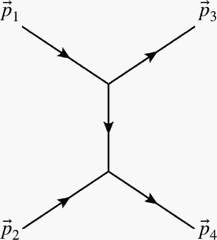
$ \phi^4 $ interaction term yields a delta function, but it is difficult to obtain numerically. Therefore, only the$ \phi^3 $ term is considered for the scattering. Perturbative theory yields the differential cross section for two-body elastic scattering$ \phi(\vec{p}_1)\phi(\vec{p}_2)\to\phi(\vec{p}_3)\phi(\vec{p}_4) $ . The Feynman diagram in Fig. 1 provides the${\rm i}\mathcal{M}$ matrix element: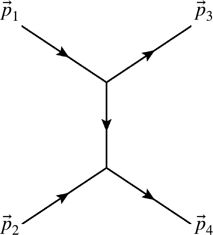
Figure 1. Feynman diagram of the t channel for elastic scattering of scalar field particles.
$ {\rm i} \mathcal{M}=(-{\rm i}\lambda_3)^2\frac{\rm i}{-(\vec{p}_3-\vec{p}_1)^2-m_g^2}=\frac{{\rm i}\lambda_3^2}{|\vec{K}|^2+m_g^2}. $

(22) Setting
$ |\vec{K}|=0 $ , we obtain the differential cross section as$ \frac{{\rm d}\sigma}{{\rm d} \Omega}=\frac{|\mathcal{M}|^2}{64\pi^2(2m_g)^2}=\frac{\lambda_3^4}{256\pi^2m_g^6}. $

(23) The
$ \phi^3 $ interaction generates a Yukawa potential in the coordinate space in non-relativistic limit. If$ V_{\mathrm{Yukawa}}(r) $ is inserted to Eq. (20), the differential cross section is expressed as$ \frac{{\rm d}\sigma}{{\rm d} \Omega}\Bigr\|_{\mathrm{Yukawa}}=\frac{Y^2}{16\pi^2m_g^2}. $

(24) Comparing Eqs. (23) and (24), we find that the value of
$ \lambda_3 $ is determined by the coefficient Y:$ \lambda_3=2m_g\sqrt{|Y|}. $

(25) The s-wave scattering cross section can also be directly extracted from the wave function. This method is grounded in the radial Schrödinger equation, in which the wave function asymptotically approaches the asymptotic form as
$ r \to \infty $ :$ \Psi(r)\xrightarrow{r\to\infty}\frac{A_{l}}{r}\sin\left[kr+\delta_l(k)\right]. $

(26) By solving the radial Schrödinger equation, we can extract the wave function
$ \Psi(r) $ and determine the phase shift$ \delta_l(k) $ . This enables the calculation of both the differential and total cross sections for the s-wave scattering in the$ k\to0 $ limit:$ \frac{{\rm d}\sigma_s}{{\rm d}\Omega} =\lim\limits_{k\to0}\frac{1}{k^2}\sin^2\left[\delta(k)\right], $

(27) $ \sigma \sim\sigma_s=4\pi\frac{{\rm d}\sigma_s}{{\rm d}\Omega}. $

(28) -
To calculate the coefficient Y in the Yukawa potential or
$ Z^{(1)} $ and$ Z^{(2)} $ in the Gaussian potential, we use the Nambu-Bethe-Salpeter (NBS) wave function derived from lattice calculations. The NBS wave function was initially developed for hadrons [57, 58] and is also suitable for analyzing glueballs. It is defined as$ \Psi_g(\vec{r})=\sum\limits_{\vec{x}}\langle0\left|\hat{O}'(0,\vec{x}+\vec{r})\hat{O}'(0,\vec{x})\right|GG\rangle, $

(29) where
$ \hat{O}' $ is a glueball operator, and$ |GG\rangle $ represents a hadron state comprising two glueballs.The NBS wave function is related to the Schrödinger equation with the interaction dark glueball potential. The spatial Schrödinger equation with a non-local potential is expressed as
$ \frac{1}{m_g}\nabla^2\Psi_g(\vec{r})=\int {\rm d}^3r^{\prime}U(\vec{r}^{\prime},\vec{r})\Psi_g(\vec{r}^{\prime}), $

(30) where
$ U(\vec{r}^{\prime},\vec{r}) $ approximates a local, central potential$ U(\vec{r}^{\prime},\vec{r})=V(r)\delta^3(\vec{r}^{\prime}-\vec{r}) $ . The relation between$ V(r) $ and$ \Psi_g(\vec{r}) $ is$ V(r)=\frac{1}{m_g}\frac{\nabla^2\Psi_g(\vec{r})}{\Psi_g(\vec{r})}. $

(31) Replacing
$ V(r) $ with Eq. (18) or (19) enables us to determine the coefficient Y or$ Z^{(1)} $ ,$ Z^{(2)} $ from$ \Psi_g(\vec{r}) $ .In lattice simulations, correlation functions to extract the NBS wave function are constructed as
$ C_g(t,\vec{r})=\sum\limits_{\vec{x}}\langle0\left|\hat{O}'(t,\vec{x}+\vec{r})\hat{O}'(t,\vec{x})\hat{S}(0,0)\right|0\rangle, $

(32) where
$ \hat{S} $ is the glueball operator source. Subsequently, the wave function is given as$ \Psi_g(\vec{r})=\lim\limits_{t\to\infty}\frac{C_g(t,\vec{r})}{C_g(t,\vec{r}=0)}. $

(33) In principle, a two-body state could serve as the source
$ \hat{S} $ . However for the dark glueball with$ J^{PC}=0^{++} $ ,$ |GG\rangle $ and$ |G\rangle $ share the same quantum numbers. Additionally, we cannot split one-body source into spatially separated correlators, unlike two- and three-body sources. Hence, we use$ \hat{S}=\hat{O}' $ . -
In this section, we present our numerical results obtained from lattice simulations. This includes an in-depth overview of the configuration generation process, the results for dark glueball mass, and the determination of the coupling coefficient for the effective Lagrangian and dark glueball scattering cross section.
-
When generating lattice configurations, we varied the coupling constant β in the set
$\{2.0,~ 2.2,~ 2.4,~ 2.6\}$ for naive actions in$S U(2)$ simulations. In contrast, for the improved actions, we specifically employed$ \beta=3.5 $ for comparative purposes.Table 1 delineates the setup of configurations employed in our study. During the generation process, we used both heatbath and overelaxation updates for the
$S U(2)$ gauge field. To enhance signal clarity, we implemented Array Processor with Emulator (APE) smearing for the gauge links, as described in [26],action β Volume heat+over Warm up Conf naive 2.0 $ 10^4 $ 

1+1 500 $ 4608 $ 

naive 2.2 $ 10^4 $ 

1+2 700 $ 4608 $ 

naive(ML) 2.2 $ 10^4 $ 

/ / $ 4608 $ 

naive 2.4 $ 16^4 $ 

1+3 700 $ 2304 $ 

naive 2.6 $ 24^4 $ 

1+5 1000 $ 1536 $ 

improved 3.5 $ 16^4 $ 

1+5 1000 $ 1536 $ 

Table 1. Setup for
$S U(2)$ lattice simulations: The initial configurations were random$S U(2)$ matrices, followed by warm-up process with heatbath updates and a production process employing combinations of one heatbath update and multiple overrelaxation updates.$ V_{\mu}(n) = U_{\mu}(n) + \alpha \sum\limits_{\pm\nu \neq \mu} U_{\nu}(n) U_{\mu}(n+\hat{\nu}) U^{\dagger}_{\nu}(n+\hat{\mu}), $

(34) $ U^{\mathrm{smear}}_{\mu}(n) = V_{\mu}(n)/\sqrt{\det{V_{\mu}(n)}}. $

(35) In our simulations, we selected a smearing parameter of
$ \alpha = 0.1 $ , and a total of 20 APE smearing iterations were uniformly applied across all configurations. Employing the established relation between the string tension σ and the scale parameter Λ as documented in [59], we determined the lattice spacing in terms of$ \Lambda^{-1} $ for each simulation setting [60]. Detailed information is given in Appendix A, and the results are listed in Table 2.action β $ a\sqrt{\sigma} $ 

$ a[\Lambda^{-1}] $ 

naive 2.0 0.6365(66) 0.3727(39) naive 2.2 0.4857(30) 0.2844(17) naive 2.4 0.2868(24) 0.1621(14) naive 2.6 0.1669(96) 0.0977(56) improved 3.5 0.3246(17) 0.1900(10) Table 2. Lattice spacings in string tension σ unit and
$S U(2)$ scale Λ for configurations of several β based on naive and improved actions.In contrast, for the ML approach, we restricted our simulations to the naive action at
$ \beta = 2.2 $ with a lattice volume of$ 10^4 $ . While ML yields configurations that closely resemble$S U(2)$ gauge configurations, they are not precise. Therefore, we used the heatbath method to update the gauge links from ML. Figure 2 compares the plaquette values from MC and ML with heatbath updates. This comparison reveals that MC configurations aligned with the ML ones after 25 heatbath updates. Eventually, we performed 40 times. Furthermore, we compared the static potentials$ aV(n_x) $ derived from large Wilson loops (see Eq. (A1)), as shown in Fig. 3. In this figure, the static potential displays a positive value of B for the$ B/r $ term, which is attributed to APE smearing. Further details are discussed in Appendix A. This comparison supports our conclusion that ML with heatbath updates can generate reasonable results as the traditional MC method.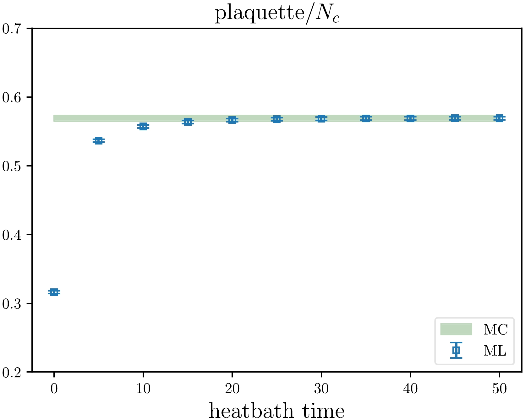
Figure 2. (color online) Comparison of plaquette based on configurations from the Monte Carlo (MC) and machine learning (ML) methods refined using the heatbath method.
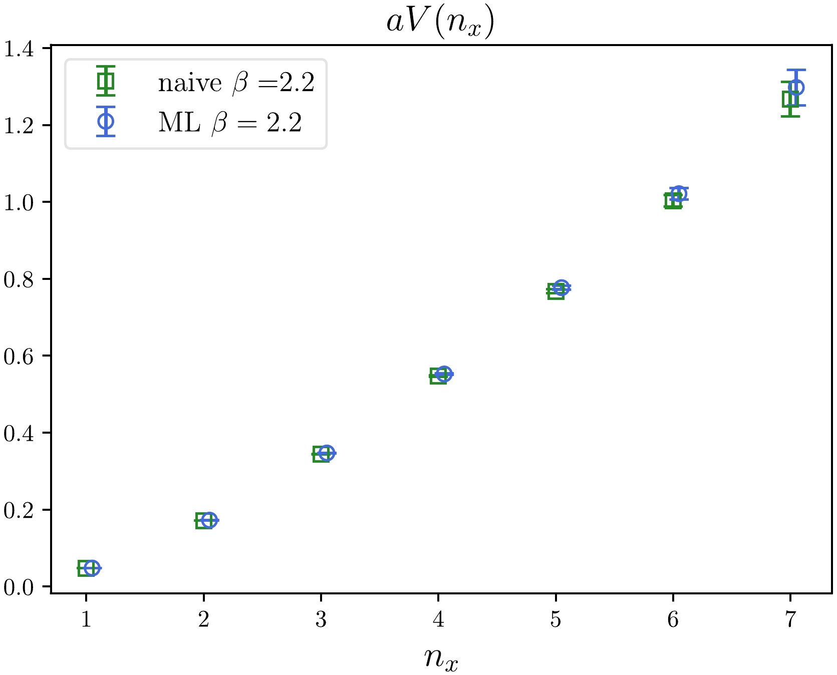
Figure 3. (color online) Comparison of static potentials from MC and ML methods with 40 times heatbath updates.
In this investigation, we also comparatively analyze the computational time consumptions of the MC and ML approaches. Note that this comparison is qualitative because, owing to the lack of GPU nodes, we used the CPU resources across six DCU nodes for the ML method. In the MC calculation for
$ 10^4 $ lattice configurations, the processing time was approximately 0.17 s per configuration. This implied that the initial warm-up process required approximately 120 s, and the total time for generation, including both warm-up and production, was calculated as (Conf$ \times $ 0.17+120) s. In contrast, the ML method involved distinct training and production phases, consuming 21 h for training and Conf$ \times $ 0.12 s for production. Figure 4 shows a cost comparison of the MC and ML methods. Based on this analysis, we can infer that the MC method is more efficient for small-scale computations, whereas ML demonstrates greater suitability for extensive-scale simulations. Therefore, in this example, configurations derived from ML exhibit reduced correlation and demand less computational time. From this perspective, ML may become an efficient method for generation.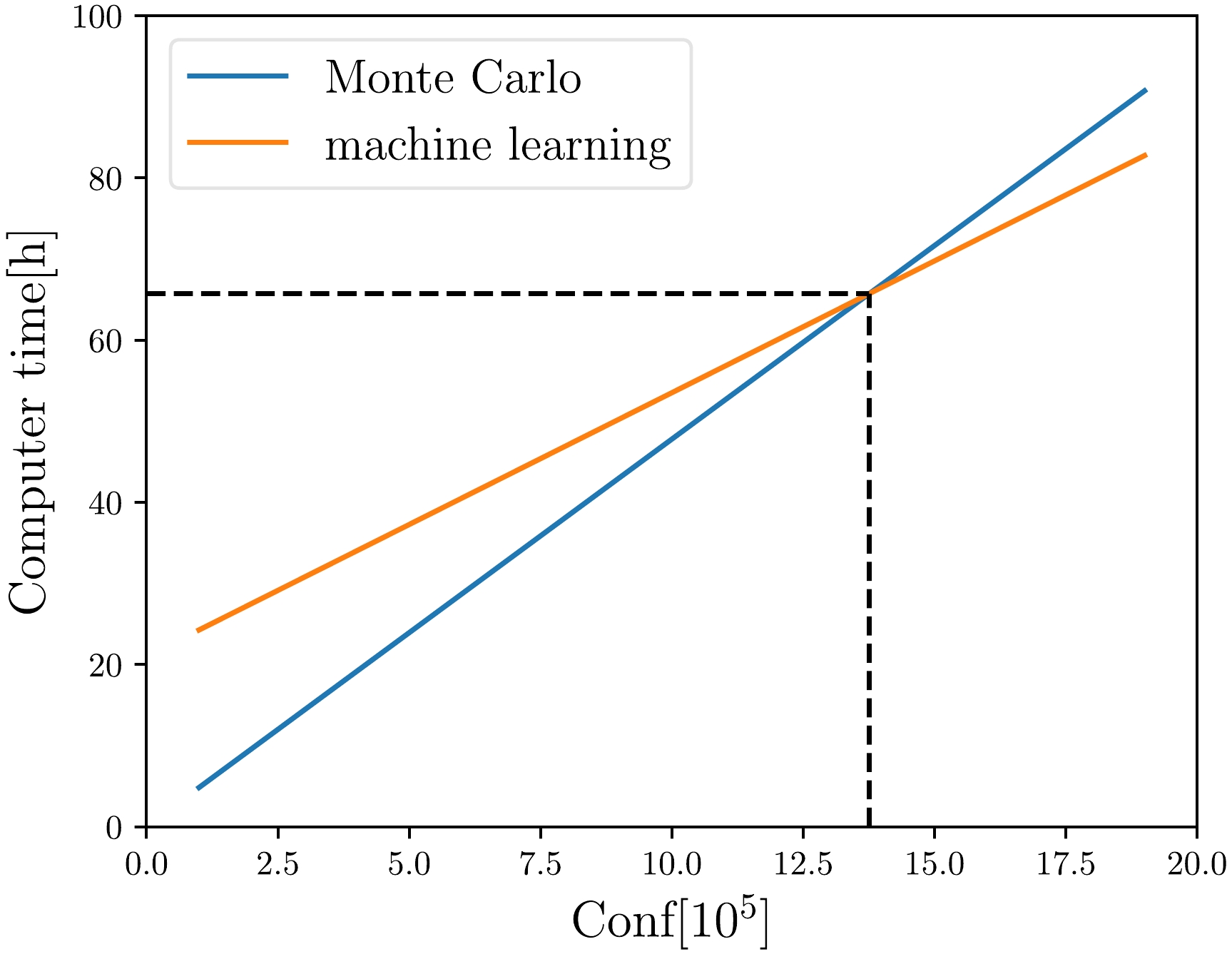
Figure 4. (color online) Comparison of computation costs of MC and ML methods.
Moreover, note that the implementation of ML is still limited. A significant problem is the large memory requirement during the training process, which may exceed the capacity of limited-core systems. Additionally, the persistent problem of mode-collapse in ML necessitates the continued use of the MC method for configuration filtering. With these considerations, our primary simulations employed the MC approach, whereas ML was utilized only for a comparative analysis at this stage.
-
The mass of the dark glueball in the framework of
$S U(2)$ gauge theory can be ascertained through the analysis of the two-point correlation function$ C_2(t) $ , as delineated in Eq. (15). Utilizing the dark glueball operator provided in Eq. (14), we select μ and ν along the spatial directions to characterize the dark glueball. Considering the ground state contribution,$ C_2(t) $ exponentially decays with respect to time slice t. Based on the periodic boundary conditions applied during the configuration generation,$ C_2(t) $ is modeled as$ C_2(t) \sim C_0 {\rm e}^{-m_gt} + C_0 {\rm e}^{-m_g(N_t-t)}. $

(36) To clearly demonstrate the value of the dark glueball mass, we present the effective mass plots in Fig. 5. Here, we calculated the effective mass
$ m^{\rm eff} $ using the following formula: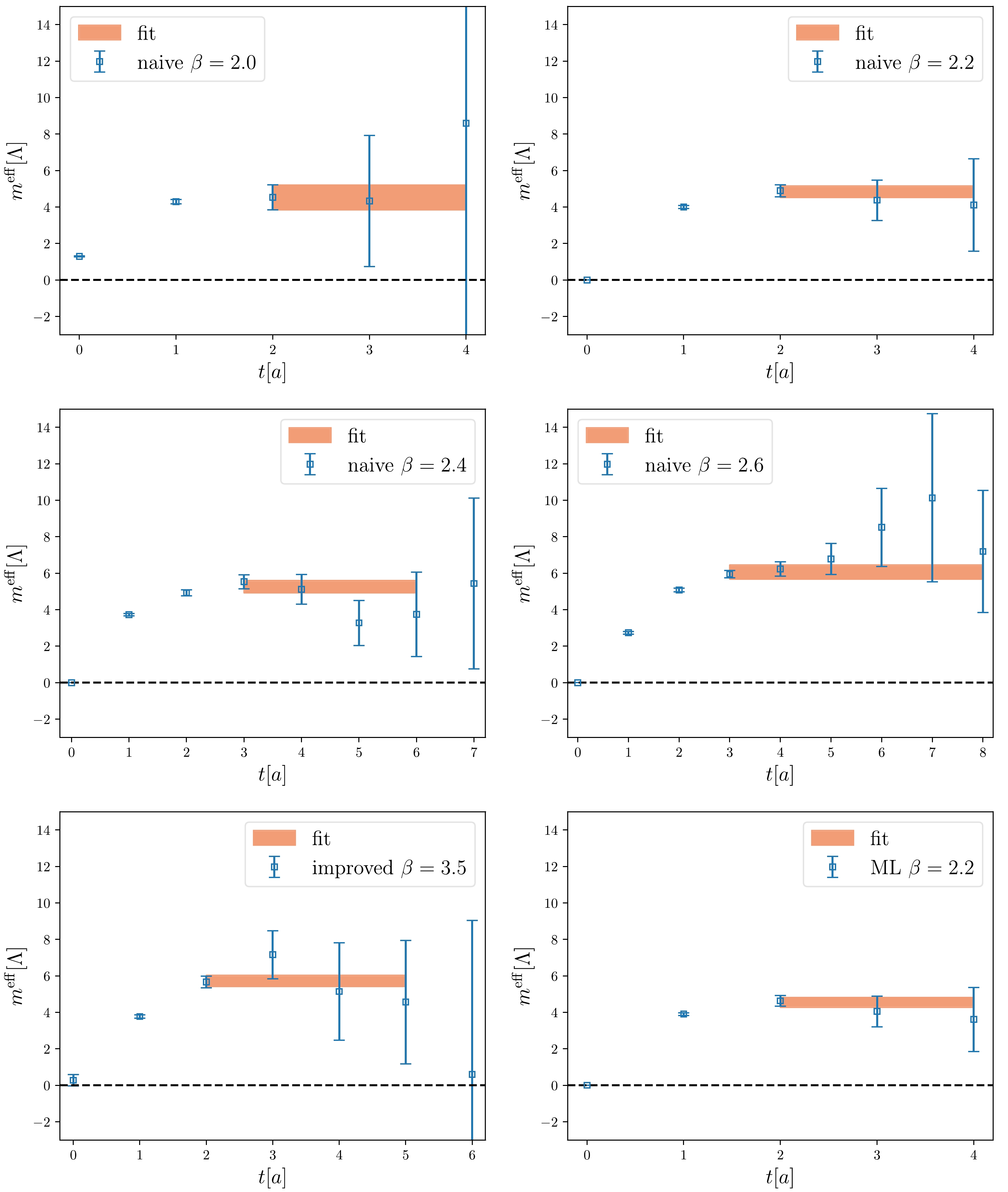
Figure 5. (color online) Effective mass plots for all cases. The corresponding fitting results are shown in Table 3. The red bands in these plots represent the fitting results, with their lengths corresponding to the fitting ranges.
$ m^{\rm eff}={\rm arccosh } \frac{C_2(t-1)+C_2(t+1)}{2C_2(t)}. $

(37) Despite considerable uncertainties in each case, the trend suggests that as t increased,
$ m^{\rm eff} $ tended to stabilize roughly towards a plateau. To enhance the stability and clarity of our fitting process, we performed a constant fit for$ m^{\rm eff} $ . The results are shown in Fig. 5 as red bands, whose lengths represent the ranges of used data in fitting. The results are also listed in Table 3, which indicates that as β increased, the dark glueball mass exhibited a gradual increase.action β $ am_g $ 

$ m_g[\Lambda] $ 

naive 2.0 1.69(25) 4.53(68) naive 2.2 1.373(89) 4.83(32) naive(ML) 2.2 1.293(77) 4.56(27) naive 2.4 0.853(54) 5.26(34) naive 2.6 0.593(17) 6.06(39) naive continuum limit / 6.35(51) improved 3.5 1.087(58) 5.72(31) Table 3. Results of effective masses of
$ 0^{++} $ glueball in lattice units and Λ.Moreover, we extrapolated the dark glueball mass to the continuum limit by using the equation
$ m^{\rm eff}_g(a) = m^{\rm eff}_g(a\to0)+c_1a+c_2a^2, $

(38) and determined the results
$ m_g(a\to0)=6.35(51)\Lambda $ . Because only the naive action was employed in the extrapolation, we retained the$ \mathcal{O}(a) $ term, which should be neglected with improved action. In parallel, our simulations using the improved action suggested an effective glueball mass of$ m_g=5.72(31)\Lambda $ . Comparing this result with those obtained using the naive action, we found that the improved action configurations at such a large lattice spacing$ a=0.1900(10)\Lambda^{-1} $ had a smaller discrete effect than naive action. We have compiled all these results in Table 3, which also shows very similar values for the naive action at$ \beta=2.2 $ , achieved through both ML and MC methods. This comparison confirms that traditional MC methods and ML techniques were consistent with each other. These results from different methods underline the usefulness of ML in particle physics, particularly for complicated tasks such as calculating the dark glueball mass. -
In this subsection, we address the determination of interaction dark glueball potentials using the NBS wave function [57, 58], as outlined in Eq. (31). Addressing the numerical second partial derivative in this context is challenging. If the potential is spherically symmetric, we can approach it by solving a radial partial differential equation:
$ \frac{{\rm d}^2R(r)}{{\rm d}r^2}+\frac{2}{r}\frac{{\rm d}R(r)}{{\rm d}r}-m_gV(r)R(r)=0, $

(39) here,
$ R(r) $ is the radial part of$ \Psi_g(\vec{r}) $ . The angular component of the solution is expressed as spherical harmonics with quantum numbers$ l,m $ , leading to$ \Psi_g(\vec{r})= R(r)Y_{l,m}(\theta,\phi) $ . Averaging$ \Psi_g(\vec{r}) $ over a spherical shell simplifies$ Y_{l,m}(\theta,\phi) $ to$ 1 $ , effectively reducing the NBS wave function$ \Psi_g(\vec{r}) $ to$ R(r) $ times a constant.To proceed, we calculate the two-body correlation function as stated in Eq. (32) and average it over spherical shells, approximating it as
$ R(r) $ . However, it is derived under the condition$ t\to\infty $ , which cannot be achieved in lattice simulations. Therefore, we examine$ R(r) $ at a fixed time separation, denoted as$ t_{\rm fix} $ , and the results are shown in Fig. 6. We observe that$ R(r) $ exhibits a modest variation with increasing t, prompting us to utilize the averaged results from several$ t_{\rm fix} $ (s). Our findings for$ R(r) $ from different lattice setups are presented in Fig. 7.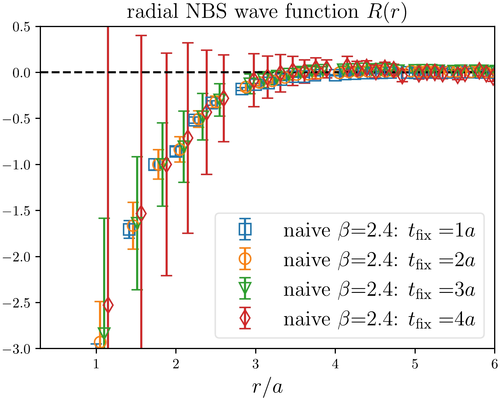
Figure 6. (color online) Radial NBS wave function
$ R(r) $ at different time separations.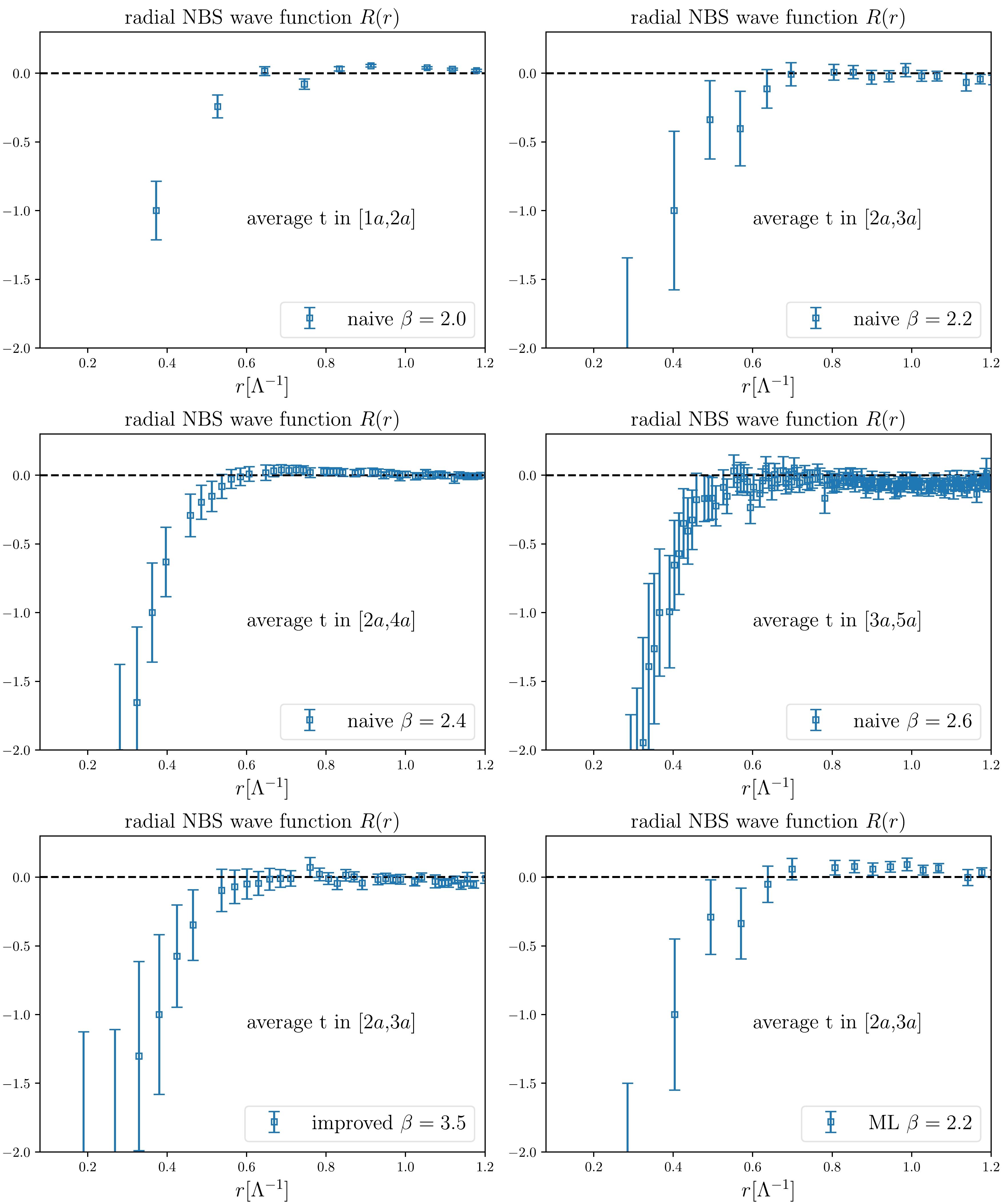
Figure 7. (color online) Radial part of the NBS wave function derived from various lattice setups. We normalize all data at
$ r=0.3727\Lambda $ and show the selected t range in the middle of each panel. As noted in the main text, the results labeled ''naive'' and ''improved'' are based on configurations with naive and improved gauge action, and ''ML'' represents results obtained with machine learning methods.Considering Yukawa and Gaussian forms of potential energy, we set boundary conditions and adjust the coefficient Y or coefficients
$ Z^{(1)} $ and$ Z^{(2)} $ to determine solutions for$ R(r) $ , denoted as$ R(r,Y) $ or$ R(r,Z^{(1)},Z^{(2)}) $ , using the fourth-order Runge-Kutta method. We then measure the differences between the$ R(r,Y) $ or$ R(r,Z^{(1)},Z^{(2)}) $ curves and the data of$ R(r) $ , selecting the curve that most closely matches our data to determine the coefficients.Figure 8 compares the solutions with Yukawa and Gaussian potentials to our lattice data. This shows that solving the differential equation Eq. (39) using the Runge-Kutta method corresponds well with our simulations, indicating reliable results. Thus, we obtained the values for Y in the Yukawa potential as well as
$ Z^{(1)} $ and$ Z^{(2)} $ in the Gaussian potential. In addition, we also investigated the$ \chi^2/\text{d.o.f} $ values of both Yukawa and Gaussian fits, finding them to be$ 2.915 $ and$ 0.764 $ , respectively, over the fitting range of$ r\in[0.4,0.9]\Lambda^{-1} $ . This indicates that the Yukawa form only partially captures the data. Consequently, we decided to increase the uncertainty of the fit parameters by a factor of$ \sqrt{\chi^2/\text{d.o.f}} $ . For clarity, we reformulate these equations as follows: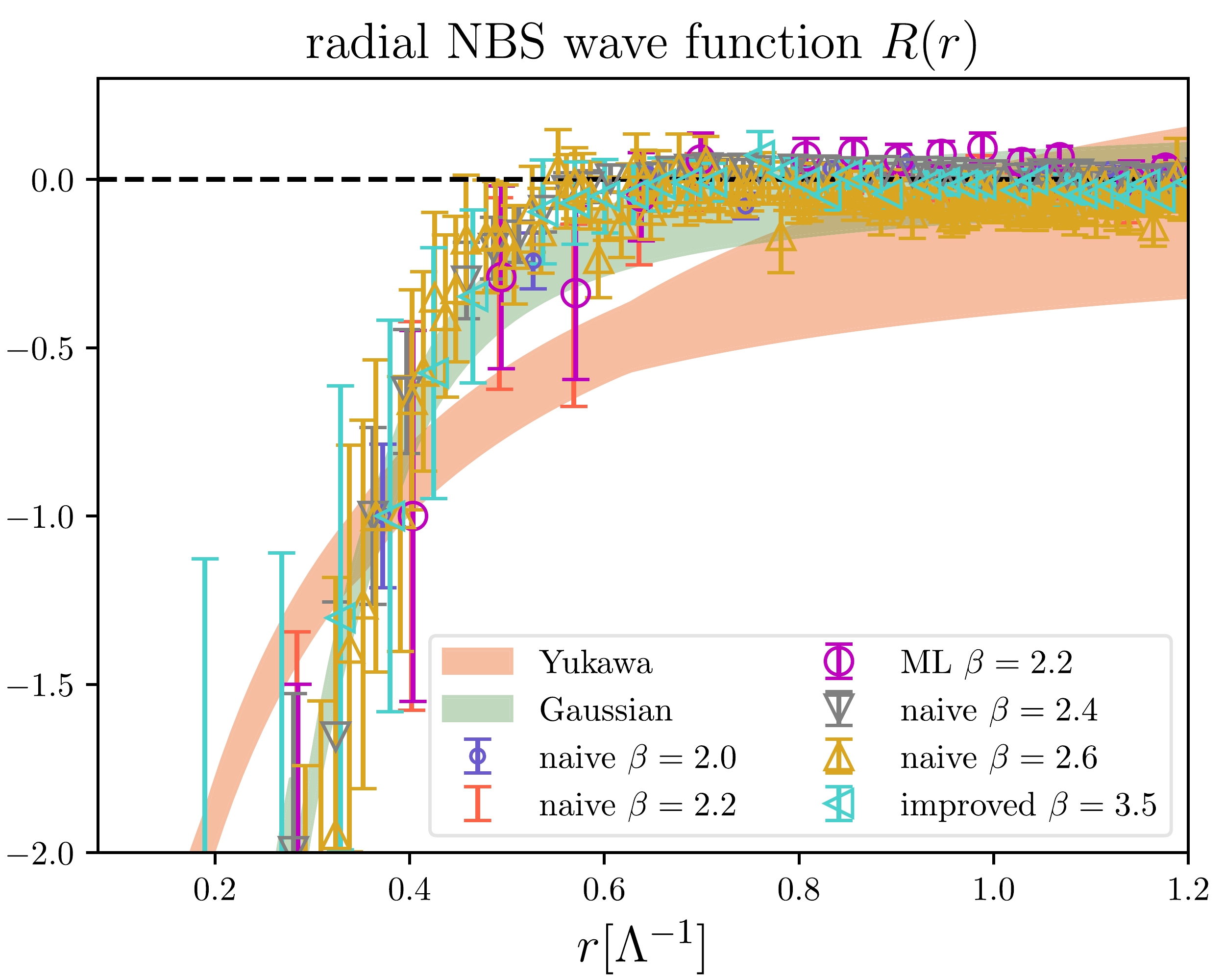
Figure 8. (color online) Results of solving the differential equation with Yukawa and Gaussian potentials.
$ V_{\mathrm{Yukawa}}(r) = -17.6(2.6)\frac{{\rm e}^{-m_gr}}{4\pi r}, $

(40) $ V_{\mathrm{Gaussian}}(r) = 12.46(0.35)\Lambda {\rm e}^{-\frac{(m_gr)^2}{8}}- 40.0(4.3)\Lambda {\rm e}^{-\frac{(m_gr)^2}{2}}. $

(41) Our current analysis shows that the Gaussian potential better matches the original data, as observed in Fig. 8. We use a combination of bands from several lattice sets for each potential, helping us to determine the final coefficients in these potentials. Through the relation between the Yukawa potential coefficient Y and the coupling coefficient
$ \lambda_3 $ in the scalar glueball Lagrangian (see Eq. (25)), we find$ \lambda_3=2m_g\sqrt{Y}=53.3(5.8)\Lambda $ .Because of these findings, we decide to use both potentials in our cross section results. We treat the difference between these two types of potential to estimate the systematic uncertainties.
Having established the values of Y,
$ Z^{(1)} $ , and$ Z^{(2)} $ , we are now equipped to formulate the Schrödinger equation for the radial wave function$ \Psi(r) $ , which is related to$ r\Psi_g(r) $ , in the presence of a non-zero relative momentum k. This equation is expressed as$ \left(\frac{{\rm d}^2}{{\rm d}r^2} + k^2 - m_gV(r)\right)\Psi(r) = 0. $

(42) When
$ r\to\infty $ ,$ V(r)\to0 $ . This suggests that$ \Psi(r) $ approaches an asymptotic form$ \Psi(r) \propto \sin(kr + \delta(k)) $ at large distances. Using the Runge-Kutta method, we can accurately solve for$ \Psi(r) $ . Applying the parameters derived from the Yukawa and Gaussian potentials, we calculate the s-wave total cross sections separately. The results with only statistic uncertainties are as follows:$ \sigma_{\mathrm{Yukawa}} = 1.110(15)\Lambda^{-2}, $

(43) $ \sigma_{\mathrm{Gaussian}} = 3.716(52)\Lambda^{-2}. $

(44) Our final result for the cross section is given as
$ \sigma = (1.09\sim3.77)\Lambda^{-2}, $

(45) which contains both statistic and systematic uncertainties.
Given our finding that both σ and
$ m_g $ vary with Λ, we can use$ m_g $ instead of Λ when representing$ \sigma/m $ . This enables us to match our$ \sigma/m $ result with experimental data and assign an appropriate value to m. Figure 9 presents our findings alongside data from experimental studies [61−64]. Our analysis shows that the ratio$ \sigma/m_g $ tends to decrease as$ m_g $ increases. Additionally, according to the current constraint, we estimate that the value of$ m_g $ is likely 0.3 GeV.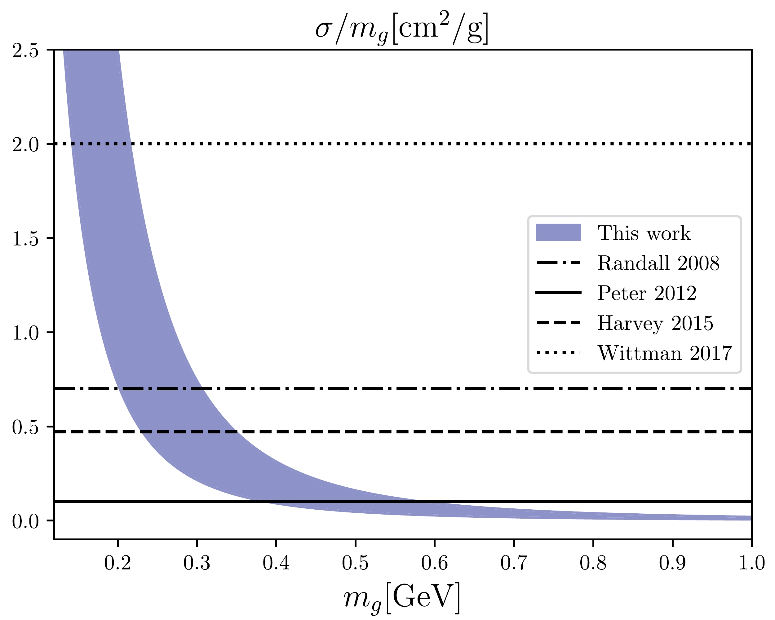
Figure 9. (color online) Ratio
$ \sigma/m_g $ against the dark glueball mass$ m_g $ . It incorporates the constraints from several researchers who have reported on the cross section of self-interacting DM. The band in the graph represents the range encompassed by our calculations. For context and comparison, the graph also includes results from established literature:$ \sigma/m=0.7 $ $ \;\mathrm{cm}^2/\mathrm{g} $ from Ref. [61],$ \sigma/m=0.1\;\mathrm{cm}^2/\mathrm{g} $ from Ref. [62],$\sigma/m= $ $ 0.47\;\mathrm{cm}^2/\mathrm{g}$ from Ref. [63], and$ \sigma/m=2.0\;\mathrm{cm}^2/\mathrm{g} $ from Ref. [64]. -
In this study, we analyze
$ 0^{++} $ glueballs within the$ S U(2) $ gauge theory using both Monte Carlo simulations and machine learning techniques. We use these two approaches to generate various lattice configurations and extract the dark glueball mass using these configurations based on naive and improved actions. Using a coupling constant of$ \beta=2.2 $ as an illustration, we compare the dark glueball mass calculated from the configurations generated from the two methods. While consistent results are achieved, the two methods demonstrate distinct advantages. Given these considerations, our primary simulations have employed the Monte Carlo approach, whereas machine learning is utilized only for a comparative analysis.Subsequently, we obtain the glueball interaction potential, which is crucial for extracting the interaction coupling constant in effective quantum field theory and determining the glueball scattering cross section. We then establish a connection between the scattering cross section and the dark glueball mass, which is a vital aspect for understanding dark glueball behavior in various physical scenarios. Our findings show that the ratio
$ \sigma/m_g $ decreases with increasing$ m_g $ , aligning with values determined in experimental studies. This correlation, along with estimated dark glueball mass$ m_g\approx0.3\;\mathrm{GeV} $ from experimental data, has significant implications for dark matter research.The application of lattice simulations to dark glueball not only reveals the potential of computational advancements in theoretical physics but also lays the foundation for more refined and efficient research methodologies in the future. Our results can contribute to the broader understanding of dark glueball dynamics and their interactions in the universe [65], particularly in relation to dark matter. This study encourages further exploration into complex particle systems and their interactions, which can be pivotal in understanding the mysteries of dark matter and its fundamental forces.
-
We are very grateful to Ying Chen, Longcheng Gui, Zhaofeng Kang, Hang Liu, Jianglai Liu, Peng Sun, Jinxin Tan, Lingxiao Wang, Yibo Yang, Haibo Yu, Ning Zhou, and Jiang Zhu for valuable discussions. The computations in this paper were run on the Siyuan-1 cluster supported by the Center for High Performance Computing at Shanghai Jiao Tong University and Advanced Computing East China Subcenter.
-
In the realm of lattice gauge theory, the expectation value of the Wilson loop is crucial. We use this value to set the lattice spacing for each lattice configuration. The static potential for the
$ S U(2) $ gauge field is determined as described in [60]:$ V(n_r) = \lim\limits_{t\to\infty}\frac{1}{a}\ln\frac{W(n_r,n_t)}{W(n_r,n_t+1)}, $

(A1) where
$ W(n_r,n_t) $ represents the Wilson loop's expectation value with length$ n_r $ and width$ n_t $ in lattice units. At short distances, this potential behaves as$ 1/n_r $ , and at larger distances, it exhibits a linear growth, represented by the string tension$ \sigma_{st} $ .In our study, we focus on the space-space Wilson loop in the
$ x-y $ plane. To represent$ aV(n_r) $ , we use the average value of$ \ln[W(n_x,n_y)/W(n_x,n_y+1)] $ over a large range of t values. As an illustration, we consider a basic setup with$ \beta=2.4 $ , depicted in Fig. A1. Here, we calculate$ aV(n_x) $ as follows: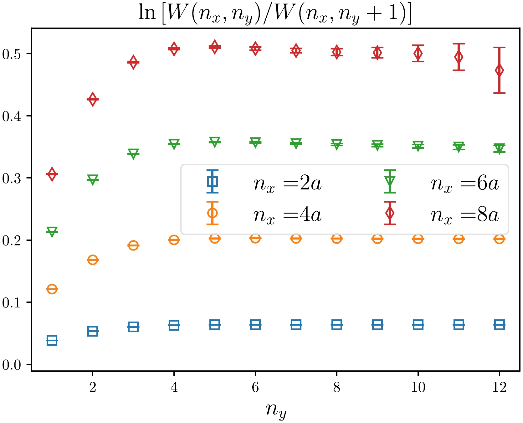
Figure A1. (color online) Plot of
$ \ln\dfrac{W(n_x,n_y)}{W(n_x,n_y+1)} $ based on naive action with$ \beta=2.4 $ .$ aV(n_x)=\frac{1}{2}\left[\ln\frac{W(n_x,8)}{W(n_x,9)}+\ln\frac{W(n_x,9)}{W(n_x,10)}\right]. $

(A2) As shown in the figure, when
$ n_y \geq 6 $ , the term$ \ln[W(n_x,n_y)/ W(n_x,n_y+1)] $ stabilizes, forming a plateau. This supports the fact that our approach is conservative.One can express
$ aV(n_x) $ as a function of$ n_x $ :$ aV(n_x) = A+\frac{B}{n_x}+a^2\sigma_{st} n_x. $

(A3) For each lattice setup, we fit the Wilson loop data to this formula to obtain the string tension
$ a^2\sigma_{st} $ . The outcomes of our fitting process are illustrated in Fig. A2, where we have selected examples with naive$ \beta=2.2 $ and$ 2.4 $ , in addition to an improved$ \beta=3.5 $ for demonstration. Fig. A2 reveals that the formula in Eq. (48) effectively captures the string tension derived from our Wilson loop data. It should be noted that, in the small spatial separation region, the term B will be influenced by APE smearing, resulting in the modification of the sign of B. However, the string tension is not significantly affected by smearing. The comparison of static potential without and with 10/20 times APE smearing is shown in Fig. A3, supporting the above observation. The effect on the lattice spacing is approximately$ (1\sim 2)\sigma $ .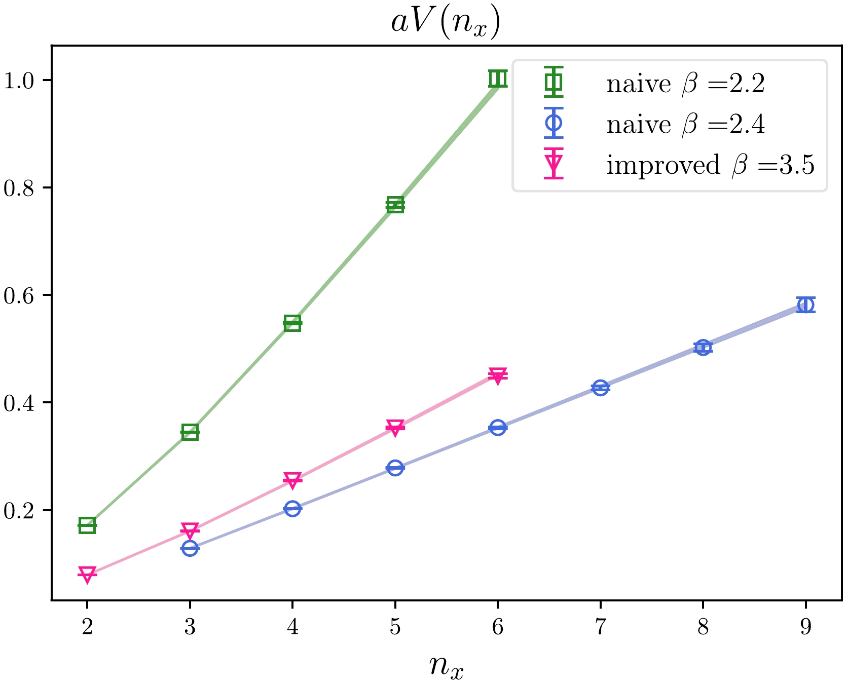
Figure A2. (color online) Fitting results for
$ aV(n_x) $ . The string tension values$ a^2\sigma_{st} $ for cases of naive$ \beta=2.2 $ and$ 2.4 $ and improved$ \beta=3.5 $ are$ 0.2359(29) $ ,$ 0.0766(13) $ , and$ 0.1053(11) $ respectively.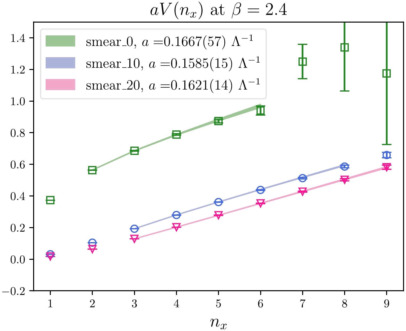
Figure A3. (color online) Static potentials from configurations with or without APE smearing at
$ \beta=2.4 $ . The number in the label after "smear_" represents times of smearing.Using the relationship between string tension and the energy scale Λ for
$S U(2)$ gauge theory [66],$ \Lambda = 0.586(45)\sqrt{\sigma_{st}}, $

(A4) we finally determine the lattice spacing in units of Λ. The results are listed in Table 2.
-
In Sec. III.C, we outline our method to determine coefficients for a specific potential using the radial wave function
$ R(r) $ , satisfying$ \frac{{\rm d}^2R(r)}{{\rm d} r^2}+\frac{2}{r}\frac{{\rm d}R(r)}{{\rm d}r}-m_gV(r)R(r)=0. $

(B1) Here,
$ V(r) $ may represent Yukawa or Gaussian potentials, each requiring one or two coefficients. Our approach is to use a test coefficient in$ V(r) $ and solve the differential equation via the Runge-Kutta method, starting from$ R(r_{\mathrm{ini}}) $ and$ R'(r_{\mathrm{ini}}) $ . The initial condition is derived from the NBS wave function of lattice data, replacing differentiation with difference.Applying the fourth-order Runge-Kutta method, we rewrite the above equation as
$ R''(r)=f(r,R,R')=\frac{2}{r}R'(r)-m_gR(r)V(r). $

(B2) Then, we can obtain the solution
$ R(r) $ by iterating the following equations with step length h:$ k_1R = hr,\;\;k_1R' = hf(r,R,R'), $

(B3) $ k_2R = h(R'+\frac{1}{2}k_1R'), $

(B4) $ k_2R' = hf(r+\frac{1}{2}h,R+\frac{1}{2}k_1R,R'+\frac{1}{2}k_1R'), $

(B5) $ k_3R = h(R'+\frac{1}{2}k_2R'), $

(B6) $ k_3R' = hf(r+\frac{1}{2}h,R+\frac{1}{2}k_2R,R'+\frac{1}{2}k_2R'), $

(B7) $ k_4R = h(R'+k_3R'), $

(B8) $ k_4R' = hf(r+h,R+k_3R,R'+k_3R'), $

(B9) $ r_1 = r+h, $

(B10) $ R_1 = R+\frac{1}{6}(k_1R+2k_2R+2k_3R+k_4R), $

(B11) $ R'_1 = R'+\frac{1}{6}(k_1R'+2k_2R'+2k_3R'+k_4R'), $

(B12) where
$ r_1 $ ,$ R_1 $ , and$ R'_1 $ are the iteratively updated values at$ r+h $ . Using test coefficients in$ V(r) $ , we approximate the corresponding solution, denoted as$ R_{\mathrm{test}}(r) $ . We then assess the distance between this test solution and our lattice data. Then, by varying the coefficients within a certain range and finding the minimal distance, we eventually identify the corresponding coefficients for$ V(r) $ .
A comparative lattice analysis of SU(2) dark glueballs
- Received Date: 2024-03-13
- Available Online: 2024-08-15
Abstract: We study the mass and scattering cross section of


 DownLoad: