


 Abstract
 HTML
HTML Reference
 Related
 PDF
PDF


-
In 2018, the BELLE Collaboration made an exciting announcement regarding the discovery of the
$ \Omega(2012) $ hyperon. This discovery was based on the$ \Omega^{*-} \to \Xi^0 K^- $ and$ \Omega^{*-} \to \Xi^- K_s^0 $ decay channels, with a measured mass of$ m = 2012.4 \pm 0.7 \,{\rm(stat)} \pm 0.6 \,{\rm(sys)}\,{\rm{MeV}} $ and decay width of$\Gamma_{\rm tot} = 6.4_{-2.0}^{+2.5} \, {\rm(stat)} \pm 1.6 \,{\rm(sys)}\,{\rm{MeV}}$ [1]. However, knowing only the mass of the state is not sufficient to determine the quantum numbers of a state. For instance, within the QCD sum rule method, the mass of the$ \Omega(2012) $ baryon is estimated, assuming it to be either the 1P or 2S excitation state [2]. Both assumptions yield the same mass value, although the estimated residues differ. Thus, additional physical quantities, such as the decay width, are necessary to identify the quantum numbers of newly discovered particles.In a previous study [3], the
$ \Omega(2012) \to \Xi^0 K^- $ transition was investigated, and its corresponding decay width was estimated by considering two possible scenarios for$ \Omega(2012) $ : either a$ 1P $ or$ 2S $ state. A comparison of the total decay widths obtained in this work led to the conclusion that$ \Omega(2012) $ is itself a$J^P = \dfrac{3}{2}^-$ state. Moreover, predictions from various theoretical models also converge on the likely quantum numbers$J^P = \dfrac{3}{2}^-$ for the observed state [4−15].In this study, considering
$ \Omega(2012) $ as the$J^P = \dfrac{3}{2}^-$ state, the strong couplings of the SU(3) partners of this state are investigated within the framework of light cone sum rules (LCSRs) using the distribution amplitudes (DAs) of the octet baryon. Note that this problem was also investigated in [16] using the flavor SU(3) symmetry approach.The structure of this paper is as follows. Section II introduces the LCSRs for the strong couplings of the transition
$\dfrac{3}{2}^- \to \dfrac{1}{2}^+$ + pseudoscalar mesons. Section III provides a numerical analysis of the LCSRs, focusing on the relevant strong couplings. Within this section, we also present the computed values of the decay widths based on the obtained coupling constants. Additionally, we compare our results with those obtained using the flavor SU(3) symmetry method. Finally, our conclusions are summarized in Section IV. -
To calculate the strong couplings of
$S U(3)$ partners, denoted as$\dfrac{3}{2}^-$ states in the following discussions, we introduce the vacuum-to-octet baryon correlation function:$ \Pi_{\mu\nu}(p,q) = {\rm i} \int {\rm d}^4x {\rm e}^{{\rm i}qx} \left\langle 0 | T\Big\{ \eta_\mu(0) J_\nu(x) \Big\} | {\cal O}(p) \right\rangle\, , $

(1) where
$ \eta_\mu $ represents the interpolating current of the decuplet baryons,$ J_\nu = \bar{q}_1 \gamma_\nu \gamma_5 q_2 $ is the interpolating current of the pseudoscalar mesons, and$ | {\cal O}(p) \rangle $ represents the octet baryon state.The interpolating current of the decuplet baryons can be written as
$ \begin{aligned}[b] \eta_\mu =\;& \varepsilon^{abc} A \Big\{ \left(q_1^{aT} C \gamma_\mu q_2^b\right) q_3^c + \left(q_2^{aT} C \gamma_\mu q_3^b \right) q_1^c \\&+ \left(q_3^{aT} C \gamma_\mu q_1^b \right) q_2^c \Big\}\; , \end{aligned} $

(2) where
$ a,b,c $ are the color indices, C is the charge conjugation operator, and A is the normalization factor. The quark content of the decuplet baryons and the normalization factor A are presented in Table 1.A $ q_1 $ 

$ q_2 $ 

$ q_3 $ 

$ \Delta^+ $ 

$\sqrt{1/3}$ 

u u d $ \Sigma^{+} (3/2) $ 

$\sqrt{1/3}$ 

u u s $ \Sigma^{0} (3/2) $ 

$\sqrt{2/3}$ 

u d s $ \Sigma^{-} $ (3/2)

$\sqrt{1/3}$ 

d d s $ \Xi^{0} $ (3/2)

$\sqrt{1/3}$ 

s s u $ \Xi^{-} (3/2) $ 

$\sqrt{1/3}$ 

s s d $ \Omega^- $ 

$ 1 $ 

s s s Table 1. Quark content of the decuplet baryons and the normalization factor A.
To derive the LCSRs for the strong coupling constants, the correlation function is computed in two ways: in terms of hadrons and in terms of quark-gluon fields within the deep Euclidean domain. By applying the quark-hadron duality ansatz, the relevant sum rules can be derived.
Strong coupling constants appear in the double dispersion relation for the correlation function given in Eq. (1). Hence, to calculate these constants, the double dispersion relation for the correlation function must be calculated. The double dispersion relation is obtained via analytical continuation of the imaginary part of the corresponding invariant amplitudes with respect to the variables
$ p^{\prime 2} $ and$ q^2 $ in the spin-3/2 and pseudoscalar meson channels, respectively.Before delving into the details of the calculations, it is important to highlight the following aspect: the interpolating current for the decuplet baryons interacts not only with the ground positive parity states
$ J^P = \dfrac{3}{2}^+ $ , but also with the negative parity states$ J^P =\dfrac{3}{2}^- $ and even with the states$ J^P = \dfrac{1}{2}^- $ .To eliminate the contributions from unwanted states,
$J^P = \dfrac{3}{2}^+$ and$J^P = \dfrac{1}{2}^-$ , a technique involving the linear contributions of different Lorentz structures is employed (for more details about this approach, refer to [17]).Following the standard procedure, we insert the total set of baryons with
$J^P = \dfrac{3}{2}$ into the correlation function along with the corresponding pseudoscalar mesons. Then, we obtain$\begin{aligned}[b] \Pi_{\mu\nu} (p,q) =\;& \sum\limits_{i=\pm} { \left\langle 0 | \eta_\mu | {3\over 2}^i (p^\prime) \right\rangle \over m_i^2 - p^{\prime 2} } \,{ \left\langle {3\over 2}^i (p^\prime) {\cal P}(q) | {\cal O}(p) \right\rangle \over m_{\cal P}^2 - q^2 } \,\\& \times \left\langle 0 | J_\nu(x) | {\cal P}(q) \right\rangle, \end{aligned} $

(3) where summation is over positive and negative states, and
$ m_{\cal P} $ is the mass of the corresponding pseudoscalar meson$ {\cal P} $ with momentum q. The matrix elements in the above equation are defined as$ \begin{aligned}[b]& \left\langle 0 \Big| \eta_\mu \Big| {3\over 2}^+ (p^\prime) \right\rangle = \lambda_+ u_\mu (p^\prime)\; , \\& \left\langle 0 \Big| \eta_\mu \Big| {3\over 2}^- (p^\prime) \right\rangle = \lambda_- \gamma_5 u_\mu (p^\prime)\; , \\ &\left\langle {3\over 2}^+ (p^\prime) {\cal P}(q) \Big| {\cal O} (p) \right\rangle = g_+ \bar{u}_\alpha (p^\prime) u(p) q^\alpha\; , \\& \left\langle {3\over 2}^- (p^\prime) {\cal P}(q) \Big| {\cal O} (p) \right\rangle = g_- \bar{u}_\alpha (p^\prime) \gamma_5 u(p) q^\alpha\; , \\& \left\langle 0 | J_\nu | {\cal P}(q) \right\rangle = {\rm i} f_{\cal P} q_\nu\; , \end{aligned} $

(4) where
$ \lambda_\pm $ are the residues of the related$\dfrac{3}{2}^\pm$ baryons,$ g_\pm $ represents the coupling constants of the$J^P = \dfrac{3}{2}^\pm$ baryons with the octet baryons and pseudoscalar mesons,$ f_{\cal P} $ is the decay constant of the pseudoscalar meson and q denotes its 4-momentum, and$ u_{\mu}(p^\prime) $ and$ u(p) $ are the Rarita-Schwinger and Dirac spinors, respectively. Performing summation over the spins of the Rarita-Schwinger spinors using the formula$ \begin{aligned}[b] \sum\limits_{s^\prime} u_\mu(p^\prime,s^\prime) \bar{u}_\alpha(p^\prime,s^\prime) =\;& - (\not {p}^\prime + m) \Bigg[ g_{\mu\alpha} - {1\over 3} \gamma_\mu \gamma_\nu \\&- {2 p_\mu^\prime p_\alpha^\prime \over 3 m^2} +{p_\mu^\prime \gamma_\alpha - p_\alpha^\prime \gamma_\mu \over 3 m} \Bigg]\; , \end{aligned} $

(5) and using Eqs. (3) and (4), we can obtain an expression for the correlation function from the hadronic part. It should be reminded that the interpolating current interacts not only with spin
$\dfrac{3}{2}$ states, but also with spin$\dfrac{1}{2}$ states.Using the condition
$ \gamma^\mu \eta_\mu=0 $ , it can easily be shown that$ \begin{array}{*{20}{l}} \left\langle 0 \Big| \eta_\mu \Big| \dfrac{1}{2} (p^\prime) \right\rangle \sim \left[ \alpha \gamma_\mu - \beta p_\mu^\prime \right] u(p^\prime)\; . \end{array} $

(6) It follows from this equation that any structure containing
$ \gamma_\mu $ or$ p_\mu^\prime $ is "contaminated" by the contributions of spin$\dfrac{1}{2}$ -states. Hence, to remove the contributions of spin$\dfrac{1}{2}$ -states, such structures are all discarded.Another problem is all Dirac structures not being independent of each other. To overcome this issue, Dirac structures must be arranged in a specific order. In this study, we choose the ordering
$\gamma_\mu \not {p}^\prime \not {q} \gamma_\nu$ .Keeping this in mind, and using Eqs. (3), (4), and (5), we obtain the correlation function from the phenomenological part as follows:
$ \begin{aligned}[b] \Pi_{\mu\nu} =\;& {\lambda_+ g_+ (- \not {q} + m_+ + m_{\cal O}) q_\mu q_\nu f_{\cal P} \over (m_+^2 - p^{\prime 2}) (m_{\cal P}^2 - q^2 )} u(p) \\&+ {\lambda_- g_- ( \not {q}+ m_- - m_{\cal O}) q_\mu q_\nu f_{\cal P} \over (m_-^2 - p^{\prime 2}) (m_{\cal P}^2 - q^2 )} u(p) + ...\; , \end{aligned} $

(7) where
$ m_{\cal O} $ is the mass of the relevant octet baryon, and$ m_+(m_-) $ is the mass of the spin-$\dfrac{3}{2}$ positive (negative) parity baryon. Here,$... $ indicates the contributions of the excited states and continuum.As a final step, we must eliminate the contributions of
$J^P = \dfrac{3}{2}^+$ states. For this purpose, the linear combinations of the invariant functions corresponding to different Lorentz structures are considered.We now turn our attention to the calculation of the correlation function using operator product expansion (OPE) in the deep Euclidean region for the variables
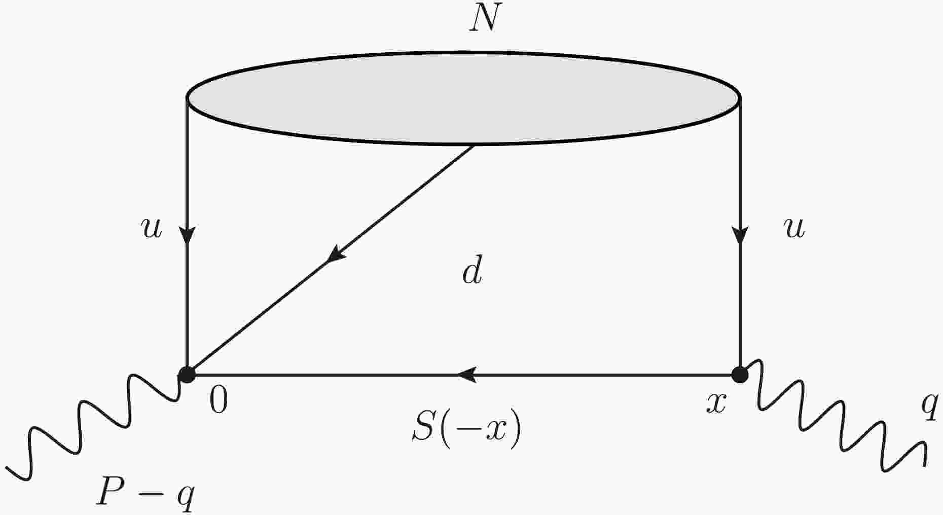
$ p^{\prime 2} = (p-q)^2 $ and$ q^2 \ll 0 $ . To calculate OPE, the explicit forms of the interpolating current are placed in the correlator, and possible contractions are performed between quark fields using Wick's theorem. As an example, for the correlation function of$ \Sigma^0 (3/2) \to N K $ , we obtain$ \begin{aligned}[b] \Pi_{\mu \nu} =\;& \sqrt{\frac{2}{3}} \int {\rm d}^4x {\rm e}^{{\rm i} q x} \epsilon_{abc} (C \gamma_\mu)_{\alpha \beta} (\gamma_\nu \gamma_5)_{\rho \sigma} \\ & \times \Big\{ \langle 0 | u_{\alpha}^a (0) u_{\sigma}^b(x) d_{\beta}^c(0) | N \rangle S_{\gamma \rho}(-x) \\ &+ \langle 0 | u_{\gamma}^c (0) u_{\sigma}^b(x) d_{\alpha}^c(0) | N \rangle S_{\beta \rho}(-x) \\ &+ \langle 0 | u_{\beta}^a (0) u_{\sigma}^b(x) d_{\gamma}^c(-x) | N \rangle S_{\alpha \rho}(-x) \Big\}, \end{aligned} $

(8) where
$ S(-x) $ is the strange quark propagator. From this expression, it follows that the OPE results are obtained via convolution of the quark propagator to the sum of the nucleon DAs, obtained from the$ \epsilon^{abc} \langle 0 | u_{\alpha}^a (0) u_{\beta}^b(x) d_{\gamma}^c(0) | N \rangle $ matrix element. A diagrammatic description of Eq. (8) is given in Fig. 1. Once we use the explicit expressions of the quark propagators and the definition of the DAs of octet baryons, the following master integral appears in the coefficients of different Lorentz structures: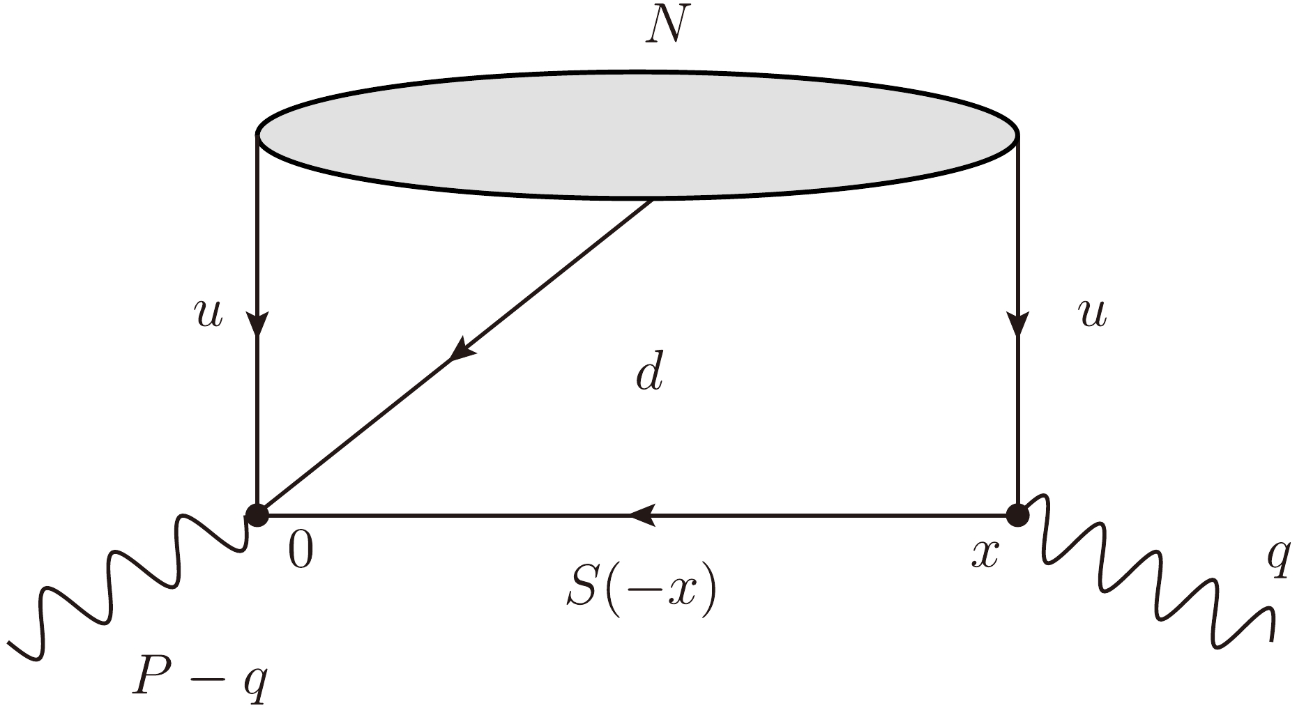
Figure 1. Diagrammatic representation of the correlation function. The wavy lines denote the external currents, solid lines correspond to the quark fields, and shaded regions correspond to the DAs of the nucleon.
$ I_{n,k} = \int {\rm d} u {u^k\over \left[m^2 - (p u - q)^2\right]^n}\; ; \; \; n=1,2,3. $

For the calculation of the double spectral densities, it is sufficient to find the double spectral representations of the master integrals. The details of the spectral density calculations for the
$ n=1 $ case are presented in Appendix A. The cases of$ n=2 $ and$ n=3 $ are calculated in a similar manner.The invariant amplitudes are related to the spectral densities via the double dispersion relation as follows:
$ \Pi[(p-q)^2,q^2] = \int {\rm d} s_1\int {\rm d} s_2 {\rho(s_1,s_2) \over [s_1-(p-q)^2] (s_2-q^2)} + \cdots $

(9) The spectral density can be obtained from
$ \Pi[(p-q)^2, q^2] $ by applying two subsequent double Borel transformations (for more details of the calculation, see Appendix A.)Matching the OPE results with the double dispersion relations for the relevant Lorentz structures of the hadrons, applying the quark-hadron duality ansatz, and performing double Borel transformation with respect to the variables
$ -(p-q)^2 $ and$ -q^2 $ , we obtain the LCSRs for the relevant coupling constants whose explicit form can be written as$ \begin{aligned}[b] g_- =\;& { {\rm e}^{m_-^2/M_1^2} \, {\rm e}^{m_{\cal P}^2/M_2^2}\over f_{\cal P} \lambda_-(m_+ +m_-) } {1\over \pi^2} \int_0^{s_0} {\rm d} s_1 \\& \times \int_{t_1(s_1)}^{\min(s_0^\prime,t_2(s_1))} {\rm d} s_2 \, {\rm e}^{-s_1/M_1^2} {\rm e}^{-s_2/M_2^2} \, {\rm I}m_{s_1} {\rm I}m_{s_2} \\& \times \Big\{\Pi_1 (m_+ - m_{\cal O}) + \Pi_2 \Big\} , \end{aligned} $

(10) where
$ \Pi_1 $ and$ \Pi_2 $ are the invariant functions of the Lorentz structures$\not {q} q_\mu q_\nu$ and$ q_\mu q_\nu $ , respectively, and$ \begin{array}{*{20}{l}} t_{1,2} = s_1 + m_{\cal O}^2 \mp 2 m_{\cal O} \sqrt{s_1-m^2}\, , \end{array} $

where m is the corresponding mass of light quarks. Here,
$ s_0^\prime $ is the continuum threshold in the pseudoscalar meson channel. The continuum threshold$ s_0^\prime $ is chosen as a mass square of the first radial excitation of the corresponding pseudoscalar meson. Finally, note that in the$ m_{\cal O} \rightarrow 0 $ limit, the applied method must be modified (for more details, see [18,19]). -
This section is devoted to the numerical analysis of the coupling constants derived in the previous section within the LCSRs. The main nonperturbative input of the considered LCSRs is the DAs of the octet baryons, namely, N, Σ, and Ξ. The explicit expressions of the relevant DAs are obtained in [20−23]. The DAs contain the normalization constants f,
$ \lambda_1 $ , and$ \lambda_2 $ , which are determined from the analysis of mass sum rules as well as lattice QCD [24, 25]. The normalization constant of the leading twist f, (for N, Σ, and Ξ baryons) is defined via the matrix element of the local current (all quark fields are at the same point).$ \begin{array}{*{20}{l}} \epsilon^{abc} \langle 0 | (q_1^{a}(0) C \not {n} q_2^{b}(0)) \gamma_5 \not {n} q_3^{c}(0) | \mathcal{O}(p) \rangle =f (pn) \not {n} u(p)\, . \end{array} $

(11) Moreover, the DAs of higher twist contributions involve two additional normalization constants,
$ \lambda_1 $ and$ \lambda_2 $ , which are defined as the matrix elements of local three quark twist-four operators,$ \begin{array}{*{20}{l}} \begin{split} \epsilon^{abc} \langle 0 | (q_1^{a}(0) C \gamma_\mu q_2^{b}(0)) \gamma_5 \gamma^\mu q_3^{c}(0) | \mathcal{O}(p) \rangle &= \lambda_1 m_{\mathcal{O}} u(p)\; , \\ \epsilon^{abc} \langle 0 | (q_1^{a}(0) C \sigma_{\mu \nu} q_2^{b}(0)) \gamma_5 \sigma^{\mu \nu} q_3^{c}(0) | \mathcal{O}(p) \rangle &= \lambda_2 m_{\mathcal{O}} u(p)\; , \end{split} \end{array} $

(12) where n is the light-like vector, and
$ u(p) $ is the Dirac bispinor.The normalization constants f,
$ \lambda_1 $ , and$ \lambda_2 $ for the Λ baryon can be obtained from Eqs. (11) and (12) via the following replacements:$ \begin{array}{*{20}{l}} & C \not {n} \to C \gamma_5 \not {n} & \gamma_5 \not {n} \to \not {n} & \quad \text{for} ~ f \end{array} $

(13) $ \begin{array}{*{20}{l}} & C \gamma_\mu \to C \gamma_5 \gamma_\mu & \gamma_5 \gamma_\mu \to \gamma_\mu & \quad \text{for}~~ \lambda_1 \end{array} $

(14) $ \begin{array}{*{20}{l}} & C \sigma_{\mu \nu} \to C \gamma_5 & \gamma_5 \sigma_{\mu \nu} \to 1 & \quad \text{for }~~ \lambda_2 \end{array} $

(15) In our analysis, we use the parameter values obtained from lattice QCD that are presented in Table 2 for completeness. The masses of the
$S U(3)$ partners of$ \Omega(2012) $ are obtained in [16] and presented below.f $ \lambda_1 $ 

$ \lambda_2 $ 

N $ 3.54 $ 

$ -44.9 $ 

$ 93.4 $ 

Σ $ 5.31 $ 

$ -46.1 $ 

$ 85.2 $ 

Ξ $ 6.11 $ 

$ -49.8 $ 

$ 99.5 $ 

Λ $ 4.87 $ 

$ -42.2 $ 

$ 98.9 $ 

Table 2. Numerical values of the parameters
$ f, \lambda_1 $ , and$ \lambda_2 $ , given in units of$ 10^{-3}\; {\rm{GeV^2}} $ .$ \begin{array}{*{20}{l}} \begin{aligned} m_- = \begin{cases} 1700 \pm 90\; {\rm{MeV}} & \text{for}\;\; \Delta , \\ 1805 \pm 100\; {\rm{MeV}} & \text{for}\;\; \Sigma(3/2) , \\ 1910 \pm 110\; {\rm{MeV}} & \text{for}\;\; \Xi(3/2), \\ 2012.4 \pm 0.9\; {\rm{MeV}} & \text{for}\;\; \Omega\; \text{[26]}. \end{cases} \end{aligned} \end{array} $

These mass values are used in our numerical analysis. For the masses of the ground state baryons, we adapt values from the PDG [26]. In addition, the value of the quark condensate is taken as
$ \langle \bar{q} q \rangle = -(246_{-19}^{+28}\; {\rm{MeV}})^3 $ [17] and$ \langle \bar{s} s \rangle = 0.8 \langle \bar{q} q \rangle $ [27].The residues of the negative parity
$J^P = \dfrac{3}{2}^-$ baryons are related to the residues of the radial excitations of the decuplet baryons as follows:$ \lambda_- = \lambda_{\rm rad} \sqrt{m_- - m_+\over m_- + m_+}\; . $

The residues of the radial excitations of the decuplet baryons are calculated in [2]. Using these results, we can easily determine the residues of the
$J^P =\dfrac{3}{2}^-$ baryons.The working regions of the Borel mass parameters and continuum thresholds,
$ s_0 $ and$ s_0^\prime $ , used in the numerical analysis are presented in Table 3. Determination of the working regions of the Borel parameters is based on the criteria that both power corrections and continuum contributions should be suppressed. Moreover, the continuum threshold$ s_0 $ is obtained under the condition that the mass of the considered states reproduces the experimental values with an accuracy of approximately 10%.Borel mass parameters Continuum threshold Continuum threshold $ M_1^2/{\rm{GeV}}^2 $ 

$ M_2^2 /{\rm{GeV}}^2 $ 

$ s_0 /{\rm{GeV}}^2 $ 

$ s_0^\prime /{\rm{GeV}}^2 $ 

$ \Delta \to N \pi $ 

$ 3 \div 4 $ 

$ 0.25 \div 0.35 $ 

$ 5.0 \pm 0.2 $ 

$ 1.7 $ 

$ \Sigma (3/2) \to N K $ 

$ 3 \div 4 $ 

$ 0.25 \div 0.35 $ 

$ 5.5 \pm 0.2 $ 

$ 2.0 $ 

$ \Sigma (3/2) \to \Lambda \pi $ 

$ 3 \div 4 $ 

$ 0.42 \div 0.44 $ 

$ 5.5 \pm 0.2 $ 

$ 1.7 $ 

$ \Sigma (3/2) \to \Sigma \pi $ 

$ 3 \div 4 $ 

$ 0.42 \div 0.44 $ 

$ 5.5 \pm 0.2 $ 

$ 1.7 $ 

$ \Xi (3/2) \to \Lambda K $ 

$ 3 \div 4 $ 

$ 0.45 \div 0.47 $ 

$ 6.0 \pm 0.2 $ 

$ 2.0 $ 

$ \Xi (3/2) \to \Sigma K $ 

$ 3 \div 4 $ 

$ 0.60 \div 0.65 $ 

$ 6.0 \pm 0.2 $ 

$ 2.0 $ 

$ \Xi (3/2) \to \Xi \pi $ 

$ 3 \div 4 $ 

$ 0.50 \div 0.60 $ 

$ 6.0 \pm 0.2 $ 

$ 1.7 $ 

$ \Omega \to \Xi K $ 

$ 3 \div 4 $ 

$ 0.55 \pm 0.65 $ 

$ 6.5 \pm 0.2 $ 

$ 2.0 $ 

Table 3. Working regions of the Borel mass parameters and continuum threshold
$ s_0 $ .Having the values of all input parameters at hand, we can perform the numerical analysis of the relevant coupling constants. As an example, in Fig. 2, we present the dependency of the coupling constant on
$ M_1^2 $ at fixed values of the continuum thresholds$ s_0 $ ,$ s_0^\prime $ , and$ M_2^2 $ for the$ \Omega \to \Xi K $ transition, because this transition has already been discovered. From this figure, we observe that there is good stability of the coupling constant when$ M_1^2 $ varies in its working region (Table 3). The obtained coupling constants are presented in Table 4. The errors in the results for the coupling constants can be attributed to the uncertainties in the input parameters as well as errors to the Borel mass parameters$ M_1^2 $ and$ M_2^2 $ and continuum threshold$ s_0 $ and$ s_0^\prime $ .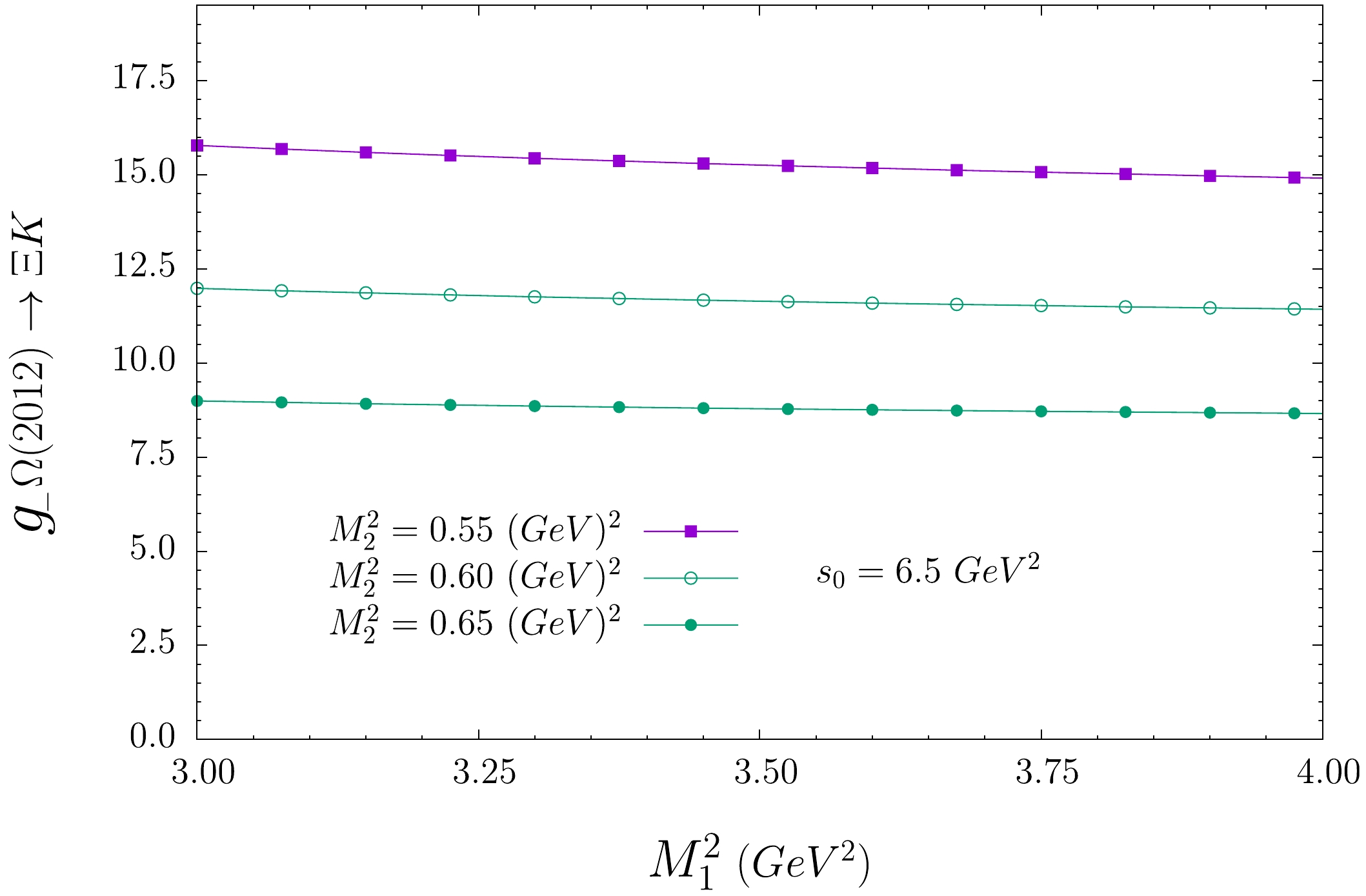
Figure 2. (color online) Dependency of the coupling constant of the
$ \Omega(2012) \to \Xi^- K^+ $ transition on the Borel mass parameter$ M_1^2 $ at several fixed values of the Borel parameter$ M_2^2 $ and the continuum threshold$s_0=6.5\;\rm GeV^2$ .Decay channels $g_-\,/{\rm{GeV} }^{-1}$ 

$\Gamma/{\rm{MeV} }$ (This study)

$\Gamma/{\rm{MeV} }$ [16]

$ \Delta \to N \pi $ 

$ 12 \pm 3 $ 

$ 71.6 \times (1.0 \pm 0.5) $ 

39−58 $ \Sigma \to N K $ 

$ 6 \pm 2 $ 

$ 11.1 \times (1.0 \pm 0.6) $ 

7−12 $ \Sigma \to \Lambda \pi $ 

$ 9 \pm 3 $ 

$ 23.7 \times (1.0 \pm 0.6) $ 

11−18 $ \Sigma \to \Sigma \pi $ 

$ 5 \pm 1 $ 

$ 4.5 \times (1.0 \pm 0.4) $ 

4−7 $ \Xi \to \Lambda K $ 

$ 10 \pm 2 $ 

$ 15.5 \times (1.0 \pm 0.4) $ 

5−10 $ \Xi \to \Sigma K $ 

$ 6 \pm 2 $ 

$ 2.7 \times (1.0 \pm 0.6) $ 

2−5 $ \Xi \to \Xi \pi $ 

$ 7 \pm 2 $ 

$ 6.9 \times (1.0 \pm 0.5) $ 

5−9 $ \Omega \to \Xi K $ 

$ 12 \pm 3.5 $ 

$ 7.4 \times (1.0 \pm 0.6) $ 

- Table 4. Decay widths of the
$J^P = \dfrac{3}{2}^-$ baryons.Having determined the coupling constants, we can calculate the decay widths of the corresponding transitions. Using the matrix elements for the considered
$\dfrac{3}{2}^- \to \dfrac{1}{2}^+ + \text{pseudoscalar meson}$ transitions, the decay width can be written as$ \Gamma = {g_-^2 \over 24 \pi m_-^2} \Big[(m_- - m_{\cal O})^2 - m_{\cal P}^2\Big] |\vec{p}|^3\; , $

(16) where
$ | \vec{p} | = {1\over 2 m_-} \sqrt{m_-^4 + m_{\cal O}^4 + m_{\cal P}^4 - 2 m_-^2 m_{\cal O}^2 - 2 m_-^2 m_{\cal P}^2 - 2 m_{\cal O}^2 m_{\cal P}^2 }\; , $

is the momentum of octet baryon, and
$ m_{\cal O} $ and$ m_{\cal P} $ are the mass of the octet baryon and pseudoscalar meson, respectively. Using the values of the coupling constants obtained within this study, we estimate the decay widths of the relevant transitions summarized in Table 4. For comparison, we also present the results of the decay widths obtained from the flavor$S U(3)$ analysis [16]. We would like to make the following remark at this point. From the expression of the decay width, it is evidently sensitive to the mass splitting among the$S U(3)$ partners of the$ \Omega(2012) $ and ground state baryons. Thus, for a fair comparison, we use the same mass values as in [16].Finally, we compare our results with the values obtained within the framework of the flavor
$S U(3)$ method [16]. In this analysis, the coupling constant for$ \Omega \to \Xi K $ is taken as the input parameter, and all the remaining couplings are expressed in terms of this coupling using$ SU(3) $ symmetry relations. Using the experimental value of the decay width$ \Omega \to \Xi K $ , we can determine the coupling constant of this transition via Eq. (16), and hence all the other coupling constants can be determined. When we compare our results on the coupling constants and decay widths of the considered decays with those obtained within the flavor$S U(3)$ analysis, we find that they are compatible within the uncertainties of the the model predictions. Small deviations in the results can be attributed to the$S U(3)$ violation effects and uncertainties of the input parameters of the theory. Furthermore, our prediction of the decay width for$ \Omega \to \Xi K $ is compatible with those observed by the BELLE Collaboration within the uncertainties [1]. Moreover, note that the coupling constant, and hence the decay width of$ \Omega \to \Xi K $ , within LCSRs method was calculated using the DAs of pseudoscalar mesons in [3]. However, in this study, we recalculate these quantities within the same framework using the DAs of the Ξ baryon. In this method, the calculations of the theoretical part of the sum rules can be achieved using only one quark propagator; however, in [3], two quark propagators were required, making the calculations difficult because each quark propagator contains many terms. Another advantage of the present method lies in dealing with the contributions of baryons with different parities, especially when mass splittings are small. In this method, no pollution arise due to negative parity baryons. However, with the methods used in [3], the problem of the separation of the contributions of positive baryons remains unsolved. Another difference between the two methods is that in this study, we consider both Borel mass parameters$ M_1^2 $ and$ M_2^2 $ but in [3],$ M_1^2 = M_2^2 $ was considered. The uncertainties of the parameters entering the DAs of baryons are larger than those of meson DAs. Once the errors are minimized in the determination of these parameters, more precise results can be obtained. When we compare our results on the coupling constant for$ \Omega \to \Xi K $ , we find that our result is consistent with that in [3] within the uncertainties. -
In conclusion, we employ the LCSR method to compute the strong coupling constants and decay widths for the
$S U(3)$ partners of the$ \Omega(2012) $ baryon in$\dfrac{3}{2}^- \to \dfrac{1}{2}^+ + \text{pseudoscalar meson}$ transitions. The "contamination" caused by the$J^P = \dfrac{3}{2}^+$ baryons are eliminated by considering the linear combinations of the sum rules obtained from different Lorentz structures. By comparing our decay width results with the findings of [16], we ascertain the compatibility of our decay width predictions with the outcomes of the flavor$S U(3)$ symmetry analysis. The small discrepancy between the predictions of the two methods may be attributed to the$S U(3)$ violation effects. Moreover, our estimated decay width for the$ \Omega \to \Xi K $ transition is also compatible with the measurement of the BELLE Collaboration within the uncertainty limits. In addition, our result on the coupling constant for$ \Omega \to \Xi K $ calculated using the DAs of Ξ is consistent with the prediction in [3], where the DAs of pseudoscalar mesons are used.Our results on the branching ratios can provide useful hints about the nature of the
$S U(3)$ partners of the$ \Omega(2012) $ baryon. -
We are grateful to Y. M. Wang for discussions on numerical analysis. We also thank A. Ozpineci for useful remarks.
-
Here, we provide the detailed derivation of the spectral density (see also [28]).
After applying the double Borel transformation over the variables
$ -{p^\prime}^2 $ and$ -q^2 $ to Eq. (9), we obtain$ \Pi^{{\cal B}_1} (M_1^2,M_2^2) = \int {\rm d}s_1 \int {\rm d}s_2 {\rm e}^{-s_1/M_1^2 -s_2/M_2^2} \rho(s_1,s_2)\; . $

(A1) Before implementing the second double Borel transformation, we introduce the new variables
$\sigma_1 = \dfrac{1}{M_i^2}$ . The second Borel transformation can be performed over the new Borel parameter$ \tau_i $ using the relation$ {\cal B}_\tau {\rm e}^{-s\sigma} = \delta\left({1\over\tau}-s\right)\; . $

(A2) As a result, we have
$ {\cal B}_{\tau_1} {\cal B}_{\tau_2} \Pi^{{\cal B}_1}(M_1^2,M_2^2) = \rho\left({1\over\tau_1},{1\over \tau_2}\right)\; . $

(A3) Hence, the double spectral density can be obtained as follows:
$ \rho(s_1,s_2) = {\cal B}_{1\over s_1}(\sigma_1) {\cal B}_{1\over s_2}(\sigma_2) \Pi^{\cal B} \left({1\over \sigma_1},{1\over \sigma_2}\right)\; . $

Let us now focus on the double spectral density for the
$ n=1 $ case. Using$ - (pu - q)^2 = -u (p-q)^2 - \bar{u} q^2 + u \bar{u} m_{\cal O}^2\; , $

where
$ \bar{u}=1-u $ ,$ I_{1,k} $ can be written as$ \begin{aligned}[b] I_{1,k} =\;& \int {\rm d} u {u^k \over \left[m^2 - u (p-q)^2 - \bar{u} q^2 + \bar{u}um_{\cal O}^2 \right]}\\=\;& \int {\rm d} u {u^k\over {\cal D}}\; , \end{aligned} $

where m is the corresponding quark mass. Using the Schwinger representation for the denominator and performing the first double Borel transformation over the variables
$ -(p-q)^2 $ and$ -q^2 $ , we obtain$ \begin{aligned}[b] I_{1,k} =\;& {\sigma_2^k \over (\sigma_1 + \sigma_2)^{k+1}} \, \exp \left[-m_{\cal O}^2 {\sigma_1 \sigma_2 \over \sigma_1 + \sigma_2} - m^2 (\sigma_1 + \sigma_2)\right]\; , \\ =\;& {\sigma_2^k \over (\sigma_1 + \sigma_2)^{k+1}} \, \exp \Bigg[m_{\cal O}^2 {\sigma_1^2 + \sigma_2^2 \over 2(\sigma_1 + \sigma_2)} - \left(m^2 + {m_{\cal O}^2 \over 2}\right)\\& (\sigma_1 + \sigma_2) \Bigg] , \end{aligned} $

where
$ \sigma_i = \dfrac{1}{M_i^2} $ . To perform the second double Borel transformation, we use the relation$ \begin{aligned}\\[-8pt] \sqrt{\sigma_1 + \sigma_2 \over 2 \pi} \int_{-\infty}^{+\infty} {\rm d} x_i \, \exp \left[{-{\sigma_1 + \sigma_2 \over 2} x_i^2 - \sigma_i m_{\cal O} x_i}\right] = \, \exp \left[{ m_{\cal O}^2 \sigma_i^2 \over 2(\sigma_1 + \sigma_2)}\right]\, . \end{aligned} $ 
Then, we obtain
$ \begin{aligned}[b] I_{1,k}^{\cal B} =\;& {1\over 2 \pi} \int_{-\infty}^{+\infty} {\rm d} x_1 \int_{-\infty}^{+\infty} {\rm d}x_2 \, {\sigma_2^k \over (\sigma_1 + \sigma_2)^k} \, \exp \Bigg[- \sigma_1 \Bigg(m^2 + {(m_{\cal O} + x_1)^2 + x_2^2 \over 2}\Bigg) - \sigma_2 \Bigg(m^2 + {(m_{\cal O} + x_2)^2 + x_1^2 \over 2}\Bigg)\Bigg]\; \\=\;& {1\over 2 \pi} {1\over \Gamma(k)} \int_{-\infty}^{+\infty} {\rm d}x_1 \int_{-\infty}^{+\infty} {\rm d}x_2\int_{0}^{\infty} {\rm d}t\, t^{k-1} \sigma_2^k \, \exp\Bigg[- \sigma_1 \Bigg(m^2 + {(m_{\cal O} + x_1)^2 + x_2^2 \over 2} + t \Bigg) - \sigma_2 \Bigg(m^2 + {(m_{\cal O} + x_2)^2 + x_1^2 \over 2} + t \Bigg)\Bigg]\; \\=\;& {1\over 2 \pi} {1\over \Gamma(k)} \int_{-\infty}^{+\infty} {\rm d}x_1 \int_{-\infty}^{+\infty} {\rm d}x_2\int_0^{\infty} {\rm d}t\, t^{k-1} \, \exp \Bigg[- \sigma_1 \Bigg(m^2 + {(m_{\cal O} + x_1)^2 + x_2^2 \over 2} + t \Bigg) \Bigg] \\&\times \Bigg( - {\partial \over \partial t}\Bigg)^k \, \exp \Bigg[ - \sigma_2 \Bigg(m^2 + {(m_{\cal O} + x_2)^2 + x_1^2 \over 2} + t \Bigg)\Bigg]\; . \end{aligned} $

After performing the second Borel transformation, we obtain the the spectral density corresponding to
$ I_{1,k} $ :$ \begin{aligned}[b] \rho_{1,k}(s_1,s_2) =\;& {1\over 2 \pi} {1\over \Gamma(k)} \Bigg(-\frac{\partial}{\partial s_2} \Bigg)^k \int_{-\infty}^{+\infty} {\rm d}x_1 \int_{-\infty}^{+\infty} {\rm d}x_2\int_0^{\infty} {\rm d}t\, t^{k-1} \delta\Bigg[ s_1 - \Bigg(m^2 + {(m_{\cal O} + x_1)^2 + x_2^2 \over 2} + t \Bigg)\Bigg]\\&\times \delta\Bigg[ s_2 - \Bigg(m^2 + {(m_{\cal O} + x_2)^2 + x_1^2 \over 2} + t \Bigg)\Bigg] \\ =\;& {1\over 2 \pi} {1\over \Gamma(k)} \Bigg( - {\partial \over \partial s_2}\Bigg)^k \int_{-\infty}^{+\infty} {\rm d}x_1 \int_{-\infty}^{+\infty} {\rm d}x_2\int_0^{\infty} {\rm d}t\, t^{k-1} \delta\Bigg[ s_1 - \Bigg(m^2 + {(m_{\cal O} + x_1)^2 + x_2^2 \over 2} + t \Bigg)\Bigg] \\&\times \delta\Bigg[ s_2 - \Bigg(m^2 + {(m_{\cal O} + x_2)^2 + x_1^2 \over 2} + t \Bigg)\Bigg] \; . \end{aligned} $

Using two Dirac delta functions, we can easily perform integrals over t and
$ x_2 $ :$ \rho_{1,k}(s_1,s_2) = {1\over 2 \pi \Gamma(k) m_{\cal O}} \Bigg( - {\partial \over \partial s_2}\Bigg)^k \int_{-\infty}^{+\infty} {\rm d}x_1 \Bigg[s_1 - \Bigg(m^2 + {(m_{\cal O} + x_1)^2 + x_2^2 \over 2} \Bigg)\Bigg]^{k-1} \Theta\Bigg[s_1 - \Bigg(m^2 + {(m_{\cal O} + x_1)^2 + x_2^2 \over 2} \Bigg)\Bigg]\; , $

where
$ x_2 = {s_2 - s_1 \over m_{\cal O}} + x_1\; , $

and
$ \Theta(x) $ is the Heaviside step function, which restricts the integral over$ x_1 $ between the limits$ y_\pm(s_1,s_2) $ , where$ y_\pm(s_1,s_2) = {- m_{\cal O}^2 + s_1 - s_2 \pm \sqrt{\Delta} \over 2 m_{\cal O}}\; , $

and
$ \begin{array}{*{20}{l}} \Delta = - m_{\cal O}^4 - (s_1-s_2)^2 + 2 m_{\cal O}^2 (-2 m^2 +s_1+s_2)\; . \end{array} $

As a result of the above summarized calculations, the spectral density can take the following form:
$ \begin{aligned}[b] \rho_{1,k}(s_1,s_2) =\;& {1\over 2 \pi} {1\over \Gamma(k)} {1\over m_{\cal O}} \Bigg( - {\partial \over \partial s_2}\Bigg)^k\\& \int_{y_-}^{y_+}{\rm d}x \Big[ (y_+-x) (x-y_-)\Big]^k \Theta(\Delta)\; . \end{aligned} $

To evaluate the x integral, we introduce a new variable through the relation
$ \begin{array}{*{20}{l}} x = (y_+-y_-) y +y_-\; , \end{array} $

so that the spectral density can be written as
$ \rho_{1,k}(s_1,s_2) = {1\over 2 \pi} {\Gamma(k)\over \Gamma(2k)} {1\over m_{\cal O}^{2 k}} \Bigg( - {\partial \over \partial s_2}\Bigg)^k \Big[\Delta^{k-{1\over 2}}\Theta(\Delta) \Big]\; . $

(A4) The double spectral densities for
$ I_{2,k} $ and$ I_{3,k} $ can be calculated using the following relations:$ I_{2,k} = \Bigg(-{\partial\over \partial m^2} \Bigg)I_{1,k}\; ,\; \rm{and,} $

$ I_{3,k} = {1\over 2} \Bigg(-{\partial\over \partial m^2}\Bigg)^2 I_{1,k}\; , $

(see also [17] for the calculation of the spectral densities
$ I_{2,k} $ and$ I_{3,k} $ ).
Analysis of strong decays of SU(3) partners of Ω(2012) baryon
- Received Date: 2024-03-26
- Available Online: 2024-08-15
Abstract: We estimate the coupling constants and decay widths of the


 DownLoad: