


 Abstract
 HTML
HTML Reference
 Related
 PDF
PDF


-
Updated mean values with estimated covariance of neutron cross sections play an important role in the advanced nuclear applications especially in the Generation-IV reactor design for its relatively higher requirement to the key targets, economy and security [1]. Evaluation methods grounded on Bayesian theory and using better physical inputs have been developed for several decades to improve existing evaluations and properly estimate not only the mean values but also the associated covariance matrices.
Great efforts have been dedicated to establishing the deterministic (Generalized Least-Squares, GLSQ) and stochastic (Monte Carlo, MC) approaches in the past to produce the consistent covariance matrix of the central values in nuclear data studies [2, 3]. The deterministic GLSQ method has been successfully introduced in the evaluations for several important databases like COMMARA-2.0 [4], BOLNA [5] and AFCI-1.2 [6], and parts of them are also adopted in the international evaluated nuclear data libraries ENDF/B-VIII.0 [7], JENDL-5 [8] and CENDL-3.2 [9]. However, some inherent problems are hard to solve due to linear approximation in GLSQ, especially when working in the model parameter space with highly-nonlinear parameter dependencies and complicated measured quantities [10].
An alternative method based on the stochastic (Monte Carlo) sampling was first proposed around 2000 by D.L. Smith et al. [11]. Various derived MC methods have been gradually developed to incorporate the nonlinear effects in the nuclear reaction study in a natural way compared to the GLSQ approach [3, 12]. However, most of the approaches only estimate the model-related uncertainties from the nuclear model parameters and lack the systematic consideration of experimental data. A Unified Monte Carlo (UMC) approach based on invoking the Bayes Theorem and the Maximum Entropy Principle from statistics was suggested to deal with this issue in 2008 [11]. Two versions UMC-G and UMC-B were proposed to adapt to different applications. UMC-G [13] works in the cross-section space and has more stringent requirements on the prior probability density function describing the theoretical calculation values of the nuclear model; UMC-B further reduces the requirement for a prior probability function, which can be non-normal or even inexpressible [14]. UMC-B is easier to be used in a realistic nuclear data evaluation.
Titanium (Ti) is one of the preferential choices for many crucial nuclear application studies [15]. The latest main evaluated libraries ENDF/B-VIII.0 [7], JEFF-3.3 [16], JENDL-5 [8] and TENDL-2021 [17] contain the covariance files for cross sections (MF=33) but covariances are not available yet in CENDL-3.2 [9]. Available covariances for selected reaction channels (MT) are listed in Table 1; the meanings of channel number MT can be found in Ref. [18]. Therefore, this paper explores the actual covariance evaluation of the neutron cross sections of the most abundant Ti isotope (48Ti) in the fast neutron energy range below 20 MeV with UMC-B, and compares the results with the existing evaluations.
Version ENDF/B-VIII.0 JEFF-3.3 TENDL-2021 JENDL-5 CENDL-3.2 Release Year 2018 2015 2019 2021 2008 First Author T. Kawano A.J. Koning A.J. Koning N. Iwamoto R. Xu Channels (MT) 1,4,16,28, 102,103,107 1-4,16,17, 22,24,28,32, 33,34,41,45, 51-54,91, 102-107,112, 115-117 1-4,16,17, 22,24,28,32, 33,34,41,45, 51-54,91, 102-107,112, 115-117 1,2,4,16, 22,28,51-91, 102-107,111 No data Method Deterministic approach with KALMAN and experimental data analysis Total Monte Carlo by TASMAN Total Monte Carlo by TASMAN Deterministic approach with KALMAN and experimental data analysis No data Table 1. Covariance evaluation in ENDF/B-VIII.0, JEFF-3.3, TENDL-2021, JENDL-5 and CENDL-3.2.
The paper is organized as follows: in Sec. II we describe the covariance evaluation formalism of UMC-B for nuclear reaction cross sections; then, in Sec. III we present the experimental data information, discuss the correlation sampling and uncertainty of nuclear model parameters and give the results and discussion for the covariance. Finally, this study is summarized in Sec. IV and the future plans are given.
-
It is known that the fast neutron reactions below 20 MeV can mainly be described with the classical theoretical models including the optical model (OM) for building a complex mean-field potential to divide the reaction flux into the shape elastic scattering and particle absorption to form the compound nucleus; the pre-equilibrium and equilibrium model for the compound nuclear decay which determine the competing particle emission channels. Nuclear reaction model is described in detail in our previous work [19], and all the current nuclear reaction calculations are performed using the Chinese nuclear reaction code UNF [20].
Nineteen parameters in total are considered in the covariance evaluation, and their central values are shown in Table 2. The parameters are explained as follows: ar, as represent the diffusive widths for the real part of the optical model potential, respectively; Rr is the radius for the real part of potential; V0, V1, V2 for depths of the real potentials; W0 for the potential of surface absorption; and U0 for depth of the potential of volume absorption. As for the compound nuclear reaction, the level density parameters and pair correction parameters for (n, inl), (n, p), (n, α), (n, γ) and (n, 2n); and the Kalbach matrix element parameter Kal to describe the two-body matrix element residual interaction, and it can control the proportion between the preequilibrium and the equilibrium process. Except the optical model potentials, all the values are taken from our previous work [19], which are also used in CENDL-3.2. The spherical optical model potential was improved to get a better fit to the neutron scattering from 48Ti in this work.
Model Parameter Central value Optical Model potential ar 0.667 (OMP) as 0.549 Rr 1.222 V0 54.398 V1 -0.498 V2 0.0068 W0 6.20 U0 -1.561 Level density (n,inelastic) 6.2 (LD) (n,p) 7.395 (n,α) 7.86 (n,γ) 6.635 (n,2n) 9.521 Pair correction (n,inelasitc) 0.01 (PC) (n,p) 0.15 (n,α) 0.1 (n,γ) 0.1 (n,2n) 0.1 Kalbach (Kal) Kal 400 Table 2. Central values of model parameters.
-
It is reported that the Unified Monte Carlo B (UMC-B) approach is an alternative compared to the original approach[21] of UMC (UMC-G) [13]. The UMC method is essentially based on Bayes' theorem and the principle of maximum entropy. The posterior probability function of target quantities is generated through involving the experimental data information (used to construct the likelihood function) and the nuclear model calculation outputs (used to construct the prior probability function). UMC-G and UMC-B differs on the fact that UMC-B estimates the Markov chain on the fly, while the UMC-G requires a calculation of a prior model PDF.
In the following derivations, the symbol “×” represents scalar multiplication, and the symbol ''·'' represents vector (or matrix) multiplication. The experimental data and their relevant covariance matrix are denoted as
$ {\bf{y}}_{E} $ and$ {\bf{V}}_{E} $ . Assume that$ {\bf{y}}_{E} $ is a n dimensional vector of the experimental data;$ {\bf{V}}_{E} $ is in n×n, which is a square, symmetrical, and positive definite matrix. The theoretical values calculated from the nuclear model are denoted by$ {\sigma}_{C} $ with m components, and its corresponding m×m dimensional covariance matrix is represented as$ {\bf{V}}_{C} $ . Similarly,$ {\bf{V}}_{C} $ is also a square, symmetrical, positive definite matrix.In this formalism, the posterior distribution function
${\boldsymbol{p}}$ of random quantity σ in Bayes theorem can be expressed as:$ p({\sigma}) = CL({\bf{y}}_{E},{\bf{V}}_{E}|{\sigma})p_0({\sigma}|{\sigma}_{C},{\bf{V}}_{C}), $

(1) where p0 is the prior probability density function;
${\boldsymbol{L}}$ is the likelihood function and${\boldsymbol{C}}$ is the normalization constant, which satisfies the normalization condition over the region of space${\boldsymbol{S}}$ to achieve convergence,$ \int_{S} p({\sigma}) \, {\rm d} {\sigma} =1, $

(2) here, the random quantity σ is composed of
$ {\sigma}_{1} $ ,$ {\sigma}_{2} $ ,...,$ {\sigma}_{i} $ ,...,$ {\sigma}_{m} $ , and its dimension is same with the theoretical quantity$ {\sigma}_{C} $ . The “best estimation” of$i-{\rm th}$ element of σ can be derived by the posterior${\boldsymbol{p}}$ as in Eq. (3)$ {\sigma}_{i}=\int_{S} {\sigma}_{i}p({\sigma}) \, {\rm d}{\sigma},\quad i=1,m, $

(3) The covariance matrix
$ {\bf{V}}_{{\sigma}} $ of the evaluated value σ is obtained with Eq. (4)$ {\rm cov} ({\sigma}_i,{\sigma}_j)=<{\sigma}_{i}{\sigma}_{j}>-<{\sigma}_{i}><{\sigma}_{j}>\quad i,j=1,m $

(4) Note that here
$ <...> $ denotes multivariate integral.It is difficult to produce the covariance matrix with equations given above. In a realistic calculation, to derive the prior probability density function p0 and the likelihood function
${\boldsymbol{L}}$ , the principle of maximum entropy by Shannon [22] and Jaynes [23] is introduced to solve the problem. The random variables can be summarized by the mean values and associated covariance matrices, and the best form to describe the prior probability density function is a multivariate normal function, namely$ p_0({\sigma}|{\sigma}_{C},{\bf{V}}_{C})\sim\exp \bigg[-\frac{1}{2}[({\sigma}-{\sigma}_{C})^T.{\bf{V}}_{C}^{-1}.({\sigma}-{\sigma}_{C})]\bigg], $

(5) $ L({\bf{y}}_{E},{\bf{V}}_{E}|{\sigma})\sim\exp\bigg[-\frac{1}{2}[({\bf{y}}-{\bf{y}}_{E})^T.{\bf{V}}_{E}^{-1}.({\bf{y}}-{\bf{y}}_{E})]\bigg], $

(6) Note that the theoretical values
$ {\bf{y}} $ and$ {\bf{y}}_{E} $ in Eq. (5) and (6) could be related by the expression$ {\bf{y}} $ =f(σ), where f represents n scalar functions$ f_{1} $ ,$ f_{2} $ ,...,$ f_{i} $ ,...,$ f_{n} $ . As a result, the posterior probability density function p(σ) can be expressed as$ \begin{aligned}[b]& p({\sigma})\sim\exp\bigg[-\frac{1}{2}[({\sigma}-{\sigma}_{C})^T.{\bf{V}}_{C}^{-1}.({\sigma}-{\sigma}_{C})\\&\quad+({\bf{y}}-{\bf{y}}_{E})^T.{\bf{V}}_{E}^{-1}.({\bf{y}}-{\bf{y}}_{E})]\bigg], \end{aligned} $

(7) where
$ [({\sigma}-{\sigma}_{C})^T.{\bf{V}}_{C}^{-1}.({\sigma}-{\sigma}_{C})+({\bf{y}}-{\bf{y}}_{E})^T.{\bf{V}}_{E}^{-1}.({\bf{y}}-{\bf{y}}_{E})]= minimum $

(8) after introducing the principle of maximum entropy, and p(σ) reaches maximum. Then, the results of UMC-B can be expressed as
$ \omega_k=\exp\bigg[-\frac{1}{2}[({\bf{y}}_k-{\bf{y}}_{E})^T.{\bf{V}}_{E}^{-1}.({\bf{y}}_k-{\bf{y}}_{E})]\bigg], $

(9) $ {\sigma}_{i} = \bigg[\sum\limits_{k=1,K} \omega_k{\sigma}_{Cik} \bigg] \Big/ \bigg[\sum\limits_{k=1,K} \omega_k\bigg],\qquad i=1,m, $

(10) $ \begin{aligned}[b]& {\rm cov} ({\sigma}_i,{\sigma}_j)= \bigg[\sum\limits_{k=1,K} \omega_k{\sigma}_{Cik}{\sigma}_{Cjk} \bigg] \Big/ \bigg[\sum\limits_{k=1,K} \omega_k\bigg]-{\sigma}_i{\sigma}_j,\\&\quad i,j=1,m, \end{aligned}$

(11) $ \omega_{k} $ is treated as a common constant for each kth sampling. The Monte Carlo history K needs to be large enough to ensure that ω values have a significant impact on the final result, so as to avoid the bias caused by the incomplete sampling. -
The present study focuses on investigating the covariance of major neutron cross sections including the total cross section (n, tot), prompt g-ray production cross section (n, γ), neutron inelastic cross section (n, inl), proton, deuterium, tritium, alpha emission cross sections (n, p), (n, d), (n, t), (n, α) and two neutron emission cross section (n, 2n) of 48Ti within the incident neutron energy (En) below 20 MeV.
In order to build the likelihood function, the experimental information of the nuclear reactions above is firstly surveyed in the EXFOR library [24]. After referring to the previous evaluation [19] and the status of measurements, we found the experimental data of three reactions (n, inl), (n, p) and (n, α) are sufficient to provide the experimental information; the experimental data of natural Ti are introduced to (n, tot) and (n, 2n) reactions to compensate the scarcity of data for 48Ti isotope. All of them are briefly listed in Table 3. The original reported uncertainties are accepted as much as possible in our work. However, since a large amount of experimental uncertainties are always missing in most of the literature, some necessary uncertainties from samples, detector, background and monitors, etc according to various experimental methods are supplemented as inputs of UMC-B. The applied data will be discussed further in Sec. IV together with the outputs of UMC-B.
Reaction Author Year Energy/MeV natTi(n,tot) W. P. Abfalterer [25] 2001 5.293-559.1 48Ti(n,inl) A. Olacel [26] 2017 0.999-17.02 48Ti(n,p) H. Lu [27] 1989 5.0-17.97 Y. Ikeda [28] 1988 13.33-14.93 Y. Ikeda [29] 1991 9.5-12 S. M. Qaim [30] 1991 5.37-10.47 H. L. Pai [31] 1966 13.6-19.5 48Ti(n,a) S. M. Qaim [30] 1991 6.48-10.47 S. M. Qaim [32] 1992 12.64-19.58 natTi(n,2n) J. Fréhaut [33] 2016 10.19-14.76 G. F. Auchampaugh [34] 1977 14.7-21 Table 3. Experimental data used in UMC-B calculation.
-
As mentioned in Sec. II, the neutron reactions of 48Ti are calculated with the theoretical calculation program UNF from 1 keV to 20 MeV, and the center values for all model parameters in Table 2. To generate the K Monte Carlo history for the eight evaluated neutron cross sections, the normal distribution is assumed for all probability functions of model parameters in sampling. In this estimation, the standard deviation of the normal distribution is assumed to be 20% for each parameter.
In the framework of the nuclear reaction models, various parameters from the optical models, level densities, and pair corrections are obviously correlated [19, 20]. An effective method to generate correlated random variables sampling sequence (with correlation coefficient matrix) based on linear transformation with Cholesky factor [35, 36] is introduced in this work, which is briefly illustrated as follows.
The target m sampling sequences for n random variables are denoted as
$ X_{m\times n} $ =($ X_{1} $ ,$ X_{2} $ ,...,$ X_{n} $ ), satisfying N-dimensional normal correlated distribution. The means and the standard deviations of these distributions are represented by$ \mu_{m\times n} $ =($ \mu_{1} $ ,$ \mu_{2} $ ,...,$ \mu_{n} $ ) and$ \eta_{m\times n} $ =($ \eta_{1} $ ,$ \eta_{2} $ ,...,$ \eta_{n} $ ) respectively. The target correlation coefficient matrix of the model parameters can be written as$ R_{n\times n} =\left[ \begin{array} {*{20}{c}} { 1 } & { r_{12} } & { ... } & { r_{1n}}\\{ r_{21} } & { 1 } & { ... } & { r_{2n}}\\{ ... } & { ... } & { ... } & { ...}\\ {r_{n1} } & { r_{n2} } & { ... } & { 1 }\end{array} \right], $

(12) $ R_{n\times n} $ is decomposed by a so-called Cholesky factor$ C_{r,n\times n} $ to make$ R_{n\times n} $ =$ C_{r,n\times n}^{\boldsymbol{T}} C_{r,n\times n} $ , noted that$ C_{r,n\times n} $ is an upper triangular matrix. Then,$ X_{m\times n} $ is finally derived through the linear transformation$ X_i = \eta_i \cdot Y_{m\times n}C_{r,n\times n}+\mu_i\qquad i=1,n, $

(13) $ Y_{m\times n} $ =($ Y_{1} $ ,$ Y_{2} $ ,...,$ Y_{n} $ ) is a sampling sequence of N-dimensional independent normally distributed random variables.Regarding to
$ R_{n\times n} $ , the nuclear reaction model parameter correlation is assumed approximately based on the empirical information from nuclear reaction calculation as in the covariance evaluation in low fidelity [37], that is,a) in the optical model: the correlation among the optical potential parameters is 50%;
b) in the compound nuclear model: the correlation among the level densities of different channels is 5%; the correlation among the pair corrections of different channels is 5%; the correlation between level density and pair correction of the same channel is 20%;
c) no correlation is considered between the optical model parameters and the compound nuclear model parameters.
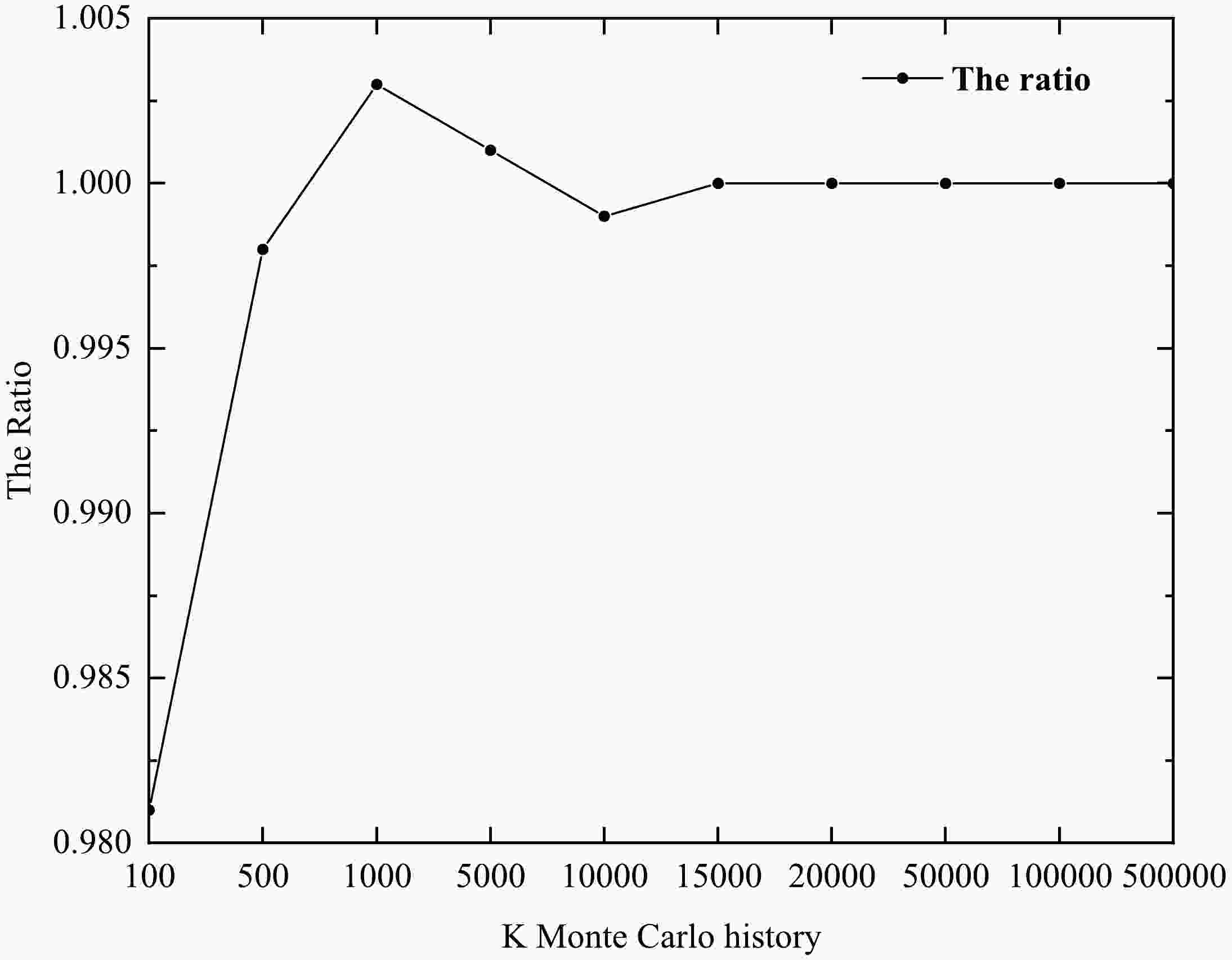
Before investigating the joint sampling for multi-parameters, the sampling convergence is discussed first. The history number K in our calculation is varied from 100, 500, 1000, 5000, 10000, 15000, 20000, 50000, 100000 to 500000 to consider this issue. To simplify the discussion, the Kalbach matrix-element parameter Kal is selected as an example here as it is assumed to be uncorrelated with other parameters. The average values and the ratios of the averages and the central values under different K samplings are shown in Fig. 1. One can conclude that the convergence can be achieved after 15000 samplings. Therefore, K = 20000 is used in our calculations to take into account the balance of stability and computing consumption. This number is also suitable for other parameters and is the one used in our calculations.
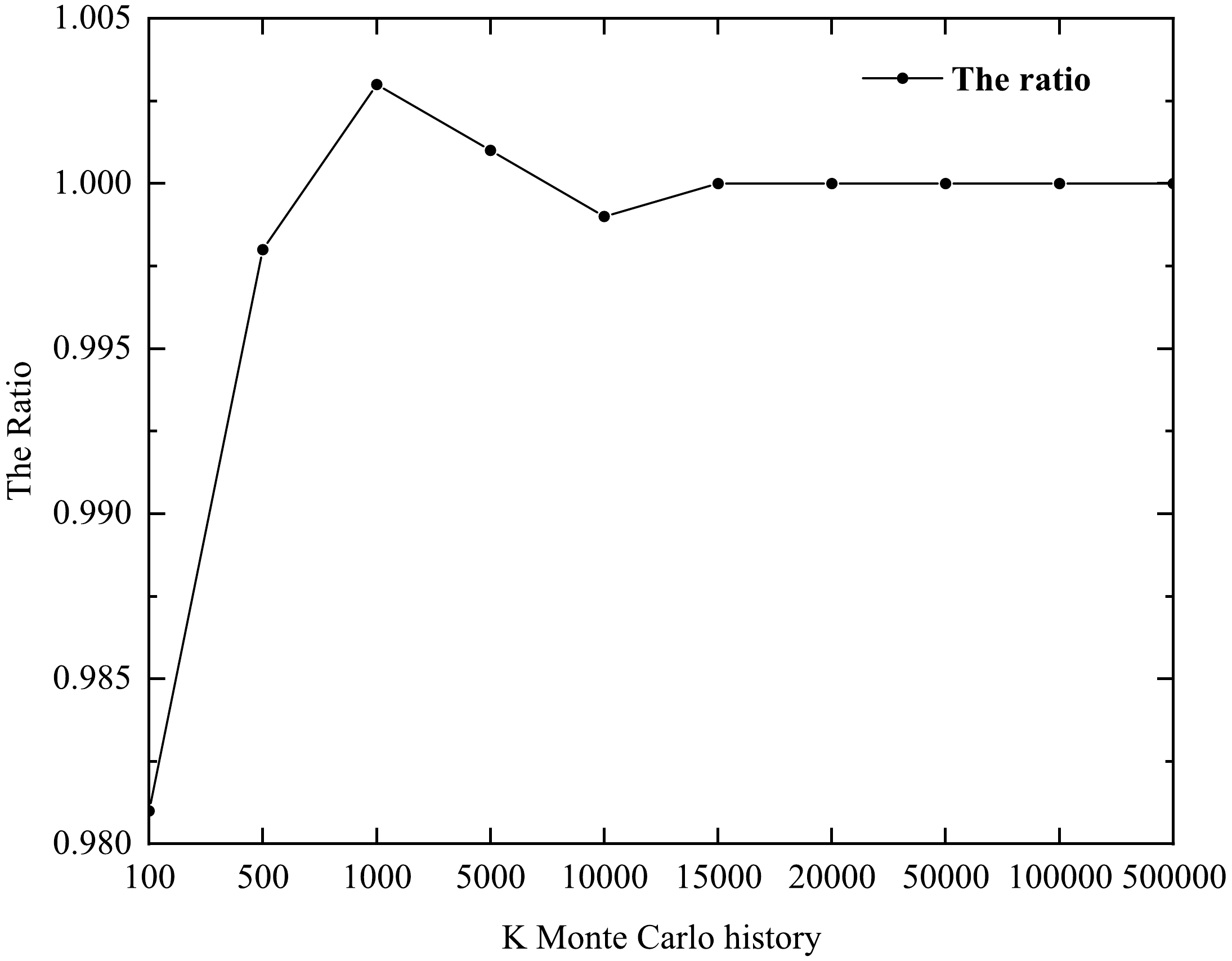
Figure 1. Ratio of sample mean to central value under different sampling histories.
The joint multi-dimensional parameter sampling is performed according to the designed
$ R_{n\times n} $ with the Cholesky approach and K = 20000 histories. As examples, Fig. 2 shows parts of the Monte-Carlo samples for the correlated level densities of different nuclear channels in Fig. 2(a), the correlated level density and pair correction of the same channel in Fig. 2(b). Slope analysis (red line in Fig. 2) estimates the correlations are 0.2 and 0.5 which satisfy the given values of$ R_{n\times n} $ . At the same time, Fig. 3 shows the comparison of the real samples of LD for (n, inl), and proposed objective normal function, and perfect coincidence is observed in the figure. As discussed above, the Cholesky factorization approach has been proved to be a very effective technique in joint sampling.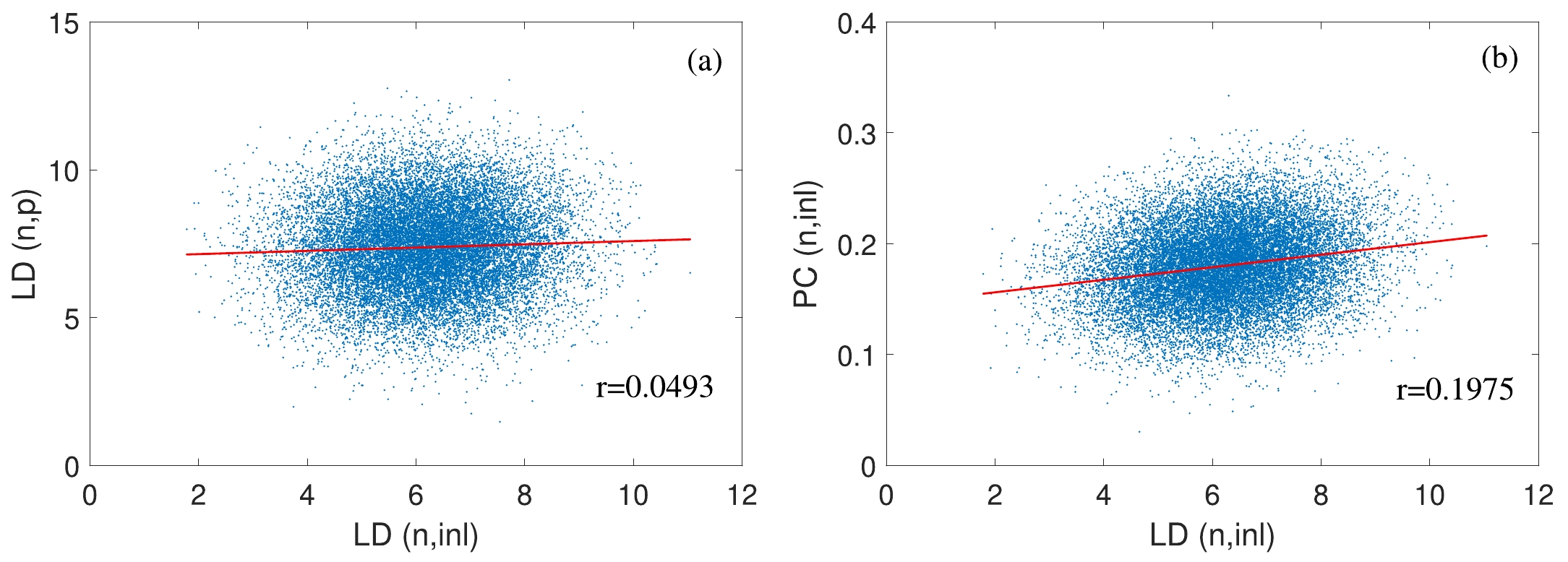
Figure 2. (color online) (a) The samples for the correlated level densities (LD) of different nuclear channels; (b) The samples for the correlated level densities (LD) and pair correction (PC) of same nuclear channel.
Figure 3. (color online) The comparison between the proposed probability with normal distribution and the real samples.
-
In order to explore the UMC-B performance with various estimated nuclear model parameter uncertainties, three calculation cases listed in Table 4 are discussed in this paper. Meanwhile, the UMC-B approach is also verified for the single nuclear reaction and the joint calculations for multi-channels in the three cases, where the (n, 2n) reaction is sampled to illustrate this systematic discussion, and two types of nuclear reaction combinations are selected as:
Case 1 Case 2 Case 3 Uncertainty OMP: 10% OMP: 30% OMP: 5% LD: 20% LD: 30% LD: 40% PC: 20% PC: 30% PC: 40% Kalbach: 30% Kalbach: 30% Kalbach: 30% Correlation OMP: 50% LD for different reactions: 5% PC for different reactions: 5% LD and PC for same reactions: 20% Table 4. Three case of nuclear model parameters uncertainty and correlation.
1) Calculation of a single reaction channel (n, 2n);
2) Joint calculations of (n, 2n) and (n, tot), (n, inl), (n, p) and (n, α), respectively.
Figure 4 shows the UMC-B results of a single reaction channel (n,2n). It can be observed that the prior theoretical value (UNF) is lower than the experimental values especially for the data from Auchampaugh [34]. The posterior results get significantly better by UMC-B in all three cases under the constraint of the concerned experimental data. This excellent ability to improve the prior curve to describe the experimental data has already been demonstrated in previous works [21].
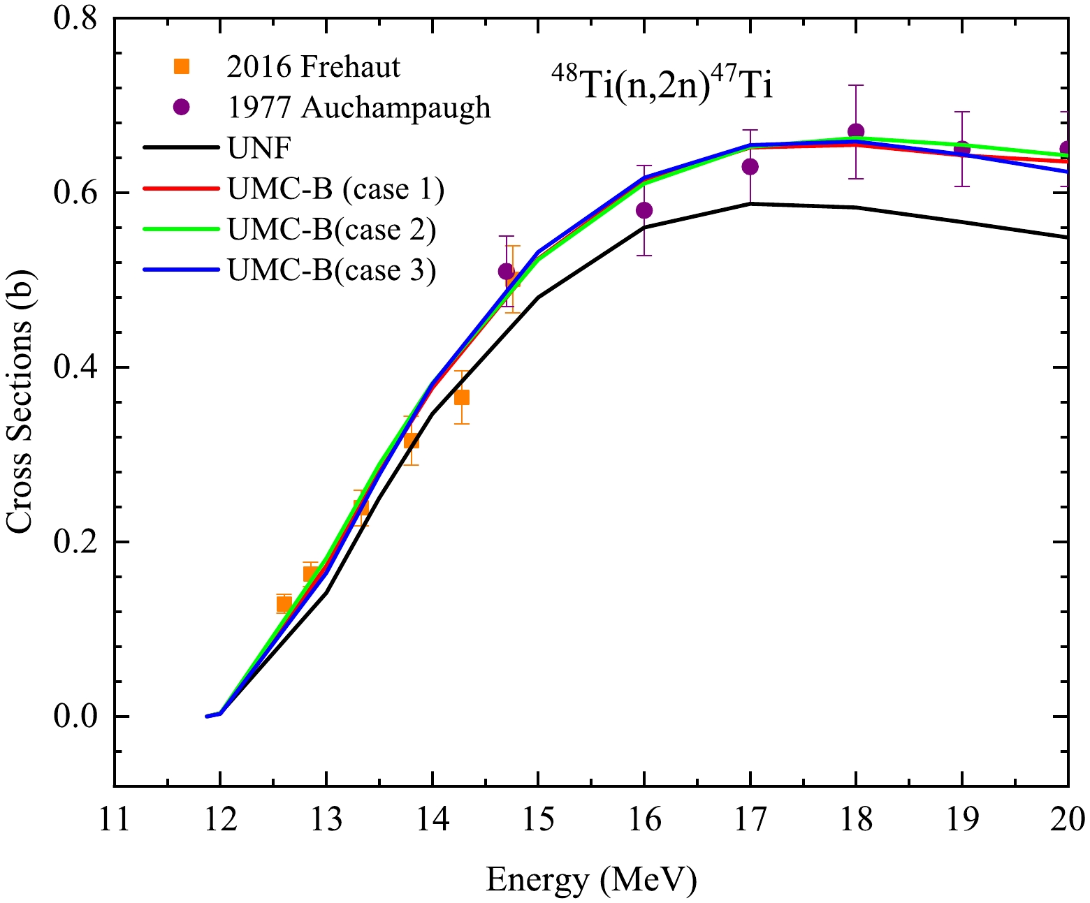
Figure 4. (color online) Comparison of UMC-B calculation results of single reaction channel in three cases.
Figure 5 exhibits the joint calculations for two channels (n, 2n) and (n, tot). For the (n, 2n) cross section, the results of case 3 is in better agreement with the experimental data, which indicates that 40% uncertainty of LD and PC is more appropriate. As for (n, tot) all cases look suitable to get good UMC-B results. Moreover, Figs. 6, Figs. 7, Fig. 8 show the joint calculations for two channels (n, 2n) with (n, inl), (n, p), and (n, α), respectively, which are competing channels involved in the compound nuclear process and the LD and PC are the main model parameters in the compound nuclear process. It can be seen that the calculated result under the condition of case 3 is more consistent with the experimental measurement, which indicates that when the uncertainties of LD and PC are larger, the experimental measurement can better constrain the theoretical value to be consistent with the experimental value.
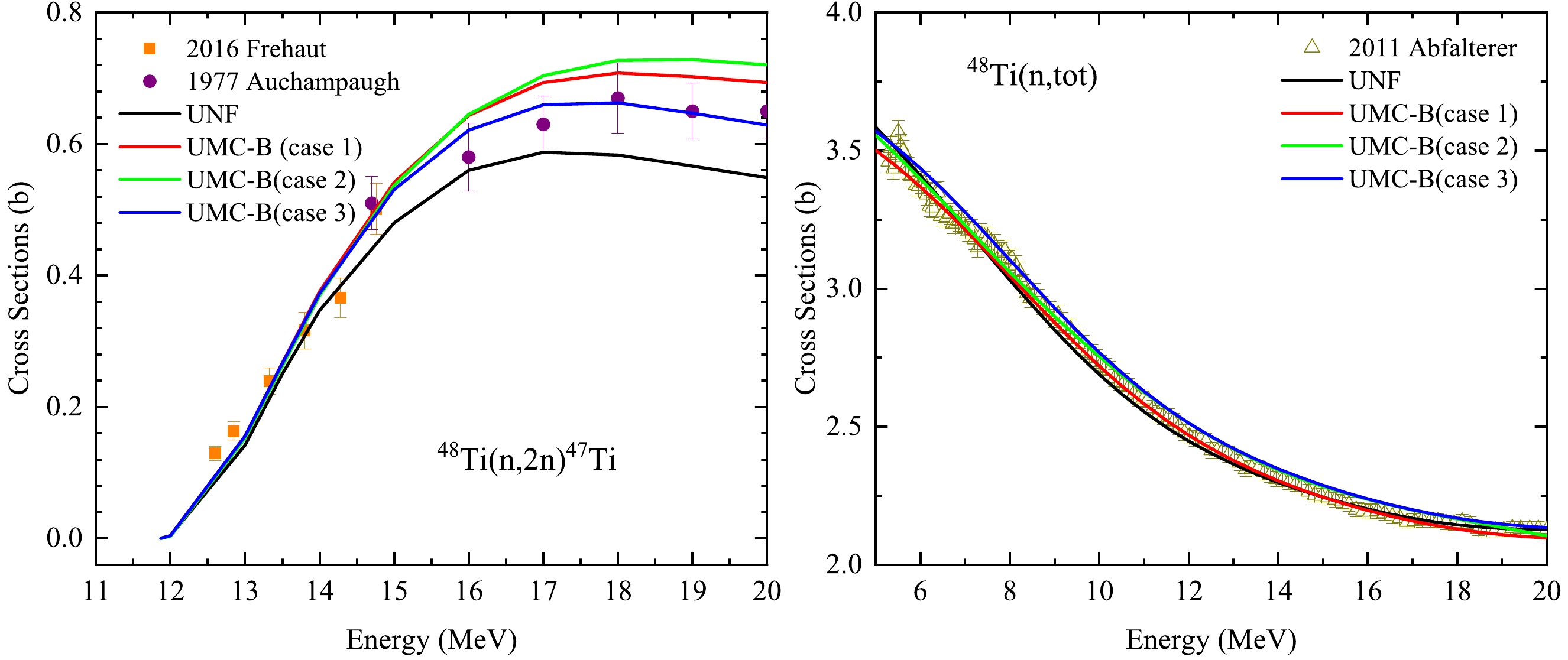
Figure 5. (color online) The UMC-B (n, 2n) and (n, tot) results under the joint calculations of (n, 2n) and (n, tot) in three cases.

Figure 6. (color online) The UMC-B (n, 2n) and (n, inl) results under the joint calculations of (n, 2n) and (n, inl) in three cases.
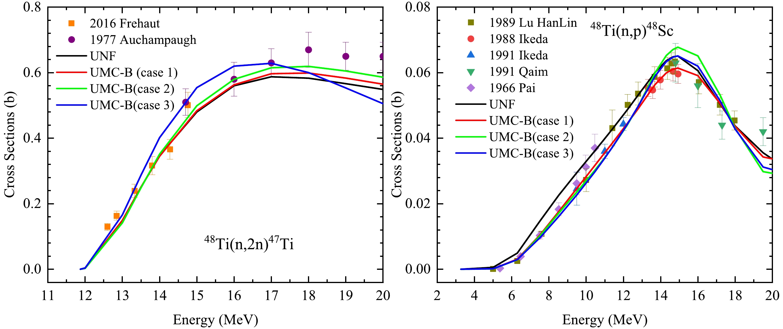
Figure 7. (color online) The UMC-B (n, 2n) and (n, p) results under the joint calculations of (n, 2n) and (n, p) in three cases.
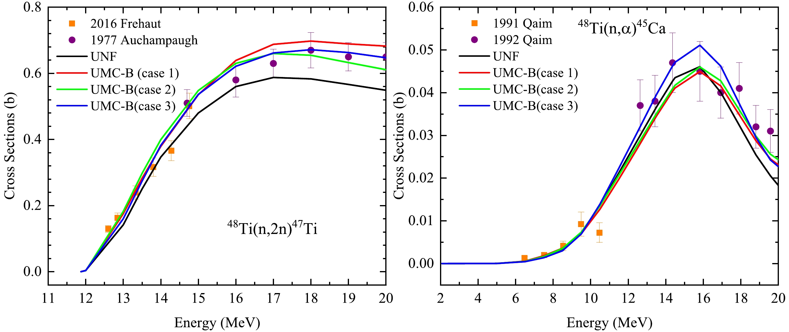
Figure 8. (color online) The UMC-B (n, 2n) and (n, α) results under the joint calculations of (n, 2n) and (n, α) in three cases.
Based on the discussion of the three cases, it can be seen that in case 3, the calculation result of single reaction channel and two reaction channels are in good agreement with the experimental data. Therefore, the nuclear model parameter uncertainties and correlations set in case 3 are adopted as the conditions for the joint calculation of eight channels.
-
The covariance matrices of eight nuclear reactions (n, tot), (n, γ), (n, inl), (n, p), (n, d), (n, t), (n, α), (n, 2n) of 48Ti in the fast neutron energy region below 20 MeV are calculated using the UMC-B approach. 19 nuclear reaction model parameters in total are involved and 20000 Monte Carlo histories are carried out for the joint multidimensional model parameter sampling. The uncertainties and correlations of the nuclear model parameters used in UMC-B (adopted case 3) are listed in Table 4. The experimental information used in the UMC-B evaluation is taken from Table 3. The evaluated cross sections and covariance are discussed in the following section.
-
In EXFOR, there is no measurement available for the channel 48Ti (n, tot). 48Ti is the most abundant isotope in natural Titanium with the abundance 73.72%, therefore we use the experimental data of natural Ti by Abfalterer et al. in the fast neutron energy region in 2001 to constrain the evaluation. Figure 9 compares the UMC-B result and the existing evaluations in CENDL-3.2, ENDF/B-VIII.0, JEFF-3.3, TENDL-2021, JENDL-5 versus experimental data. It is observed that the current theoretical curve of (n, tot) cross sections (black one) with the evaluated absolute uncertainty (light red band) cover the evaluations of other libraries and Abfalterer’s data in the left panel in Fig. 9. Meanwhile, the evaluations in JENDL-5 and JEFF-3.3 adopt the resonance structures of experimental data in Fig. 9, and our current curve keeps smooth shape which is originated from the theoretical nuclear reaction calculations. We do not expect an impact on applications of these differences. Our inputted experimental relative uncertainties (RU) are almost constant and populated around 1.2% in the right panel, and all evaluated RUs are larger than the measured ones and less than 6%. The two evaluations in ENDF/B-VIII.0, JENDL-5 via the deterministic approaches and the evaluations in JEFF-3.3, TENDL-2021 via the stochastic approaches are all obviously separated from each other. The present results with UMC-B also shows deviations from others, and our RU decreases for En
$ > $ 10 MeV, which could benefit from the abundant measurements of other channels in this energy region as shown in Table 3. At the same time, the correlation matrix (CM) in UMC-B looks pretty similar to other libraries, but we used a denser incident energy grid, as shown in Fig. 10.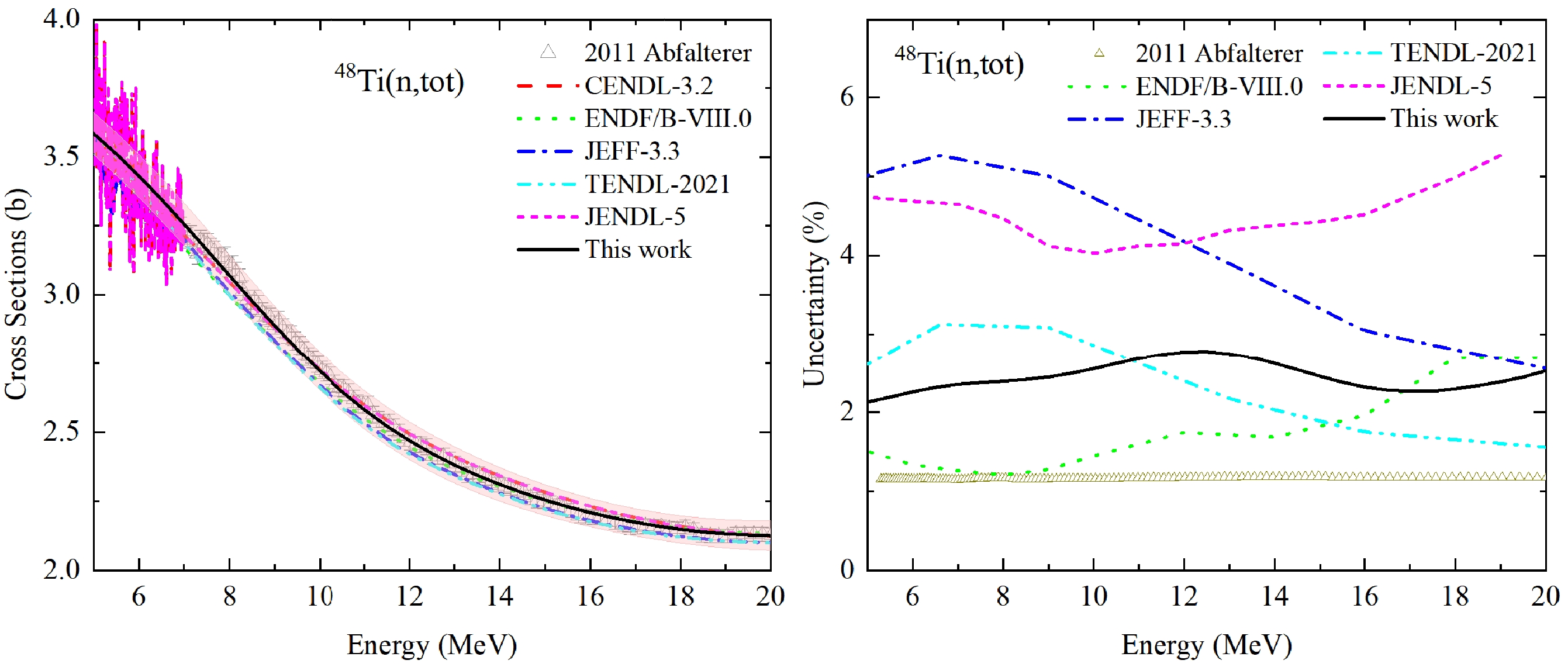
Figure 9. (color online) Comparisons of (n, tot) cross sections and uncertainties with the evaluations in ENDF/B-VIII.0, JEFF-3.3, TENDL-2021, this evaluation and the experiment data.
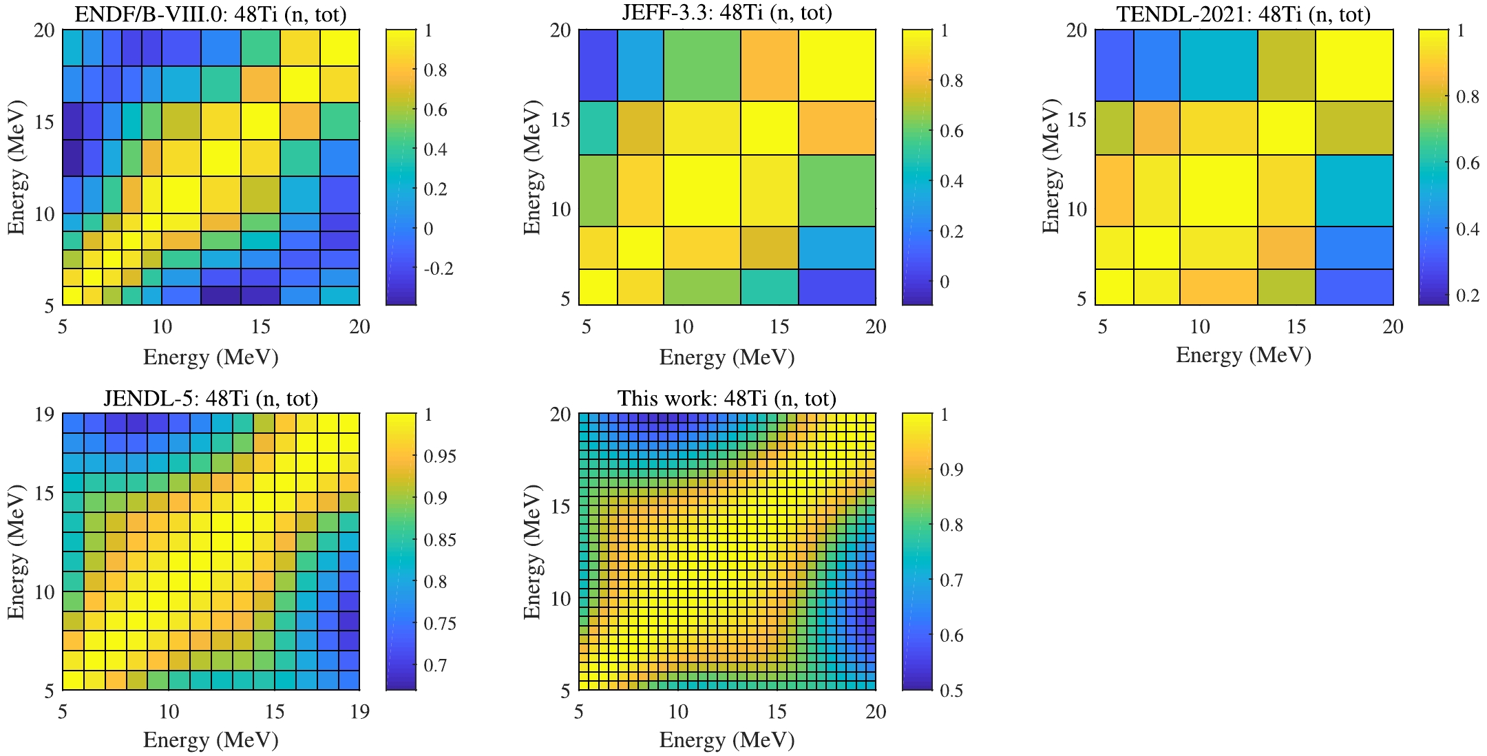
Figure 10. (color online) Comparison of the correlation coefficient matrices for (n, tot) in ENDF/B-VIII.0, JEFF-3.3, TENDL-2021, JENDL-5 and this work.
-
Neutron inelastic reaction (n, inl) is one of the most important competing channels in the fast neutron energy region. Both OMP and compound nuclear reaction model parameters will affect this reaction. Similar analysis is performed for (n, inl) in Fig. 11 and Fig. 12. The experimental data of isotope 48Ti from A. Olacel et al. is considered. The uncertainties of UMC-B generally cover all evaluations and measurements except CENDL-3.2. The derived RU is smaller than the evaluations of the libraries and inputted experimental information in Fig. 11, meaning that the prior model uncertainties were underestimated. However, the evaluated posterior cross section (n, inl) slightly overestimates the measurements from A. Olacel et al. around En = 4−8 MeV. . This overestimation deserves further study. Meanwhile, the CC matrix also follows the trend observed in other evaluations in ENDF/B-VIII.0 in Fig. 12.
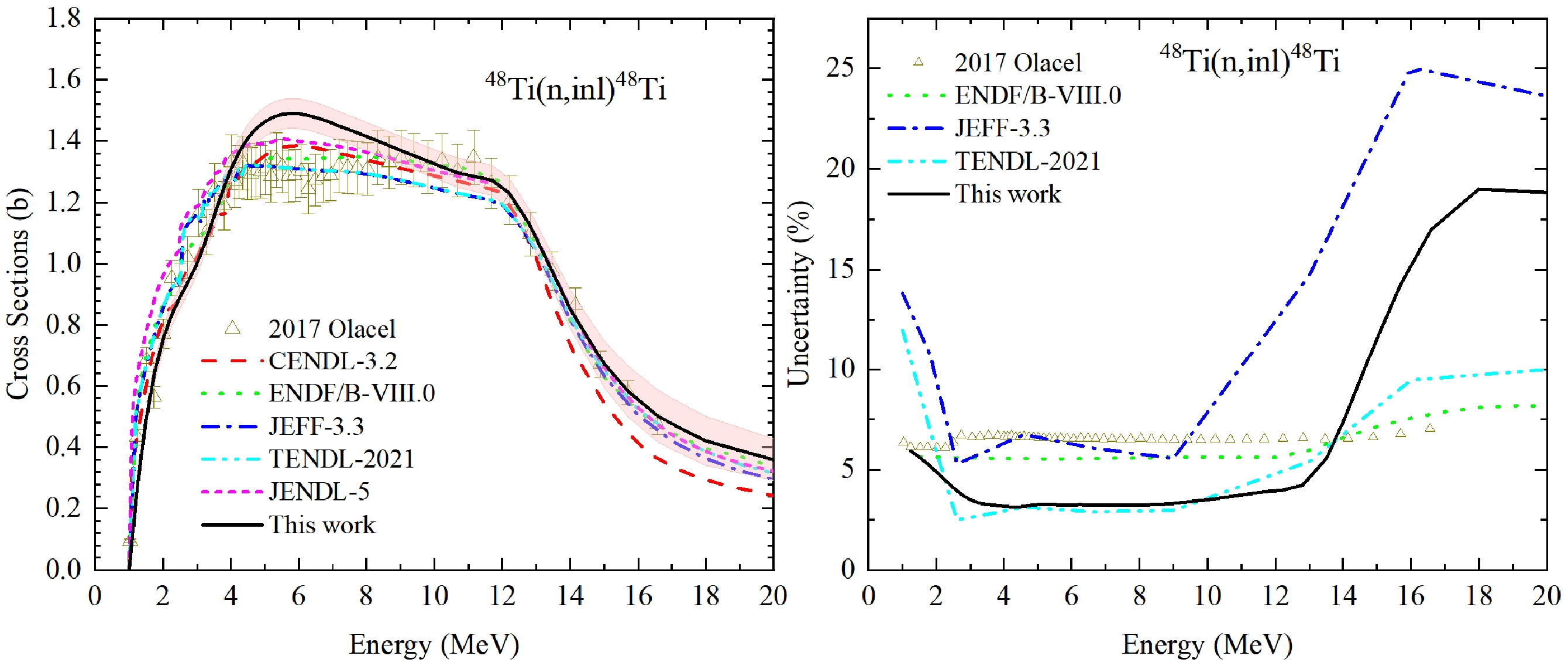
Figure 11. (color online) Comparisons of (n, inl) cross sections and uncertainties with the evaluations in CENDL-3.2, ENDF/B-VIII.0, JEFF-3.3, TENDL-2021, JENDL-5, this evaluation and the experiment data.
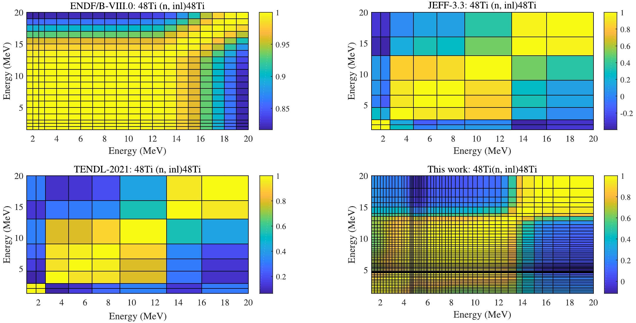
Figure 12. (color online) Comparison of the correlation coefficient matrices for (n, inl) in ENDF/B-VIII.0, JEFF-3.3, TENDL-2021 and this work.
-
Five sets of experimental data of isotope 48Ti are selected for this reaction. The input RUs of these measurements are shown in the right panel of Fig. 13, and our derived uncertainties can also cover the other evaluations and the experimental data in the left panel in Fig. 13. In Fig. 14, one can observe that the CM of UMC-B show larger correlations than CMs in ENDF/B-VIII.0 and JENDL-5.
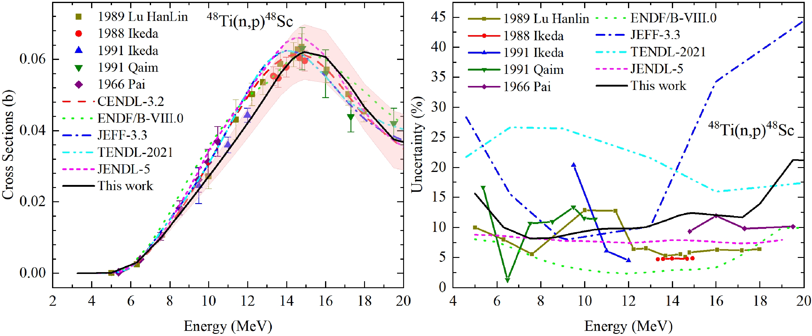
Figure 13. (color online) Comparisons of (n, p) cross sections and uncertainties with the evaluations in CENDL-3.2, ENDF/B-VIII.0, JEFF-3.3, TENDL-2021, JENDL-5, this evaluation and the experiment data.
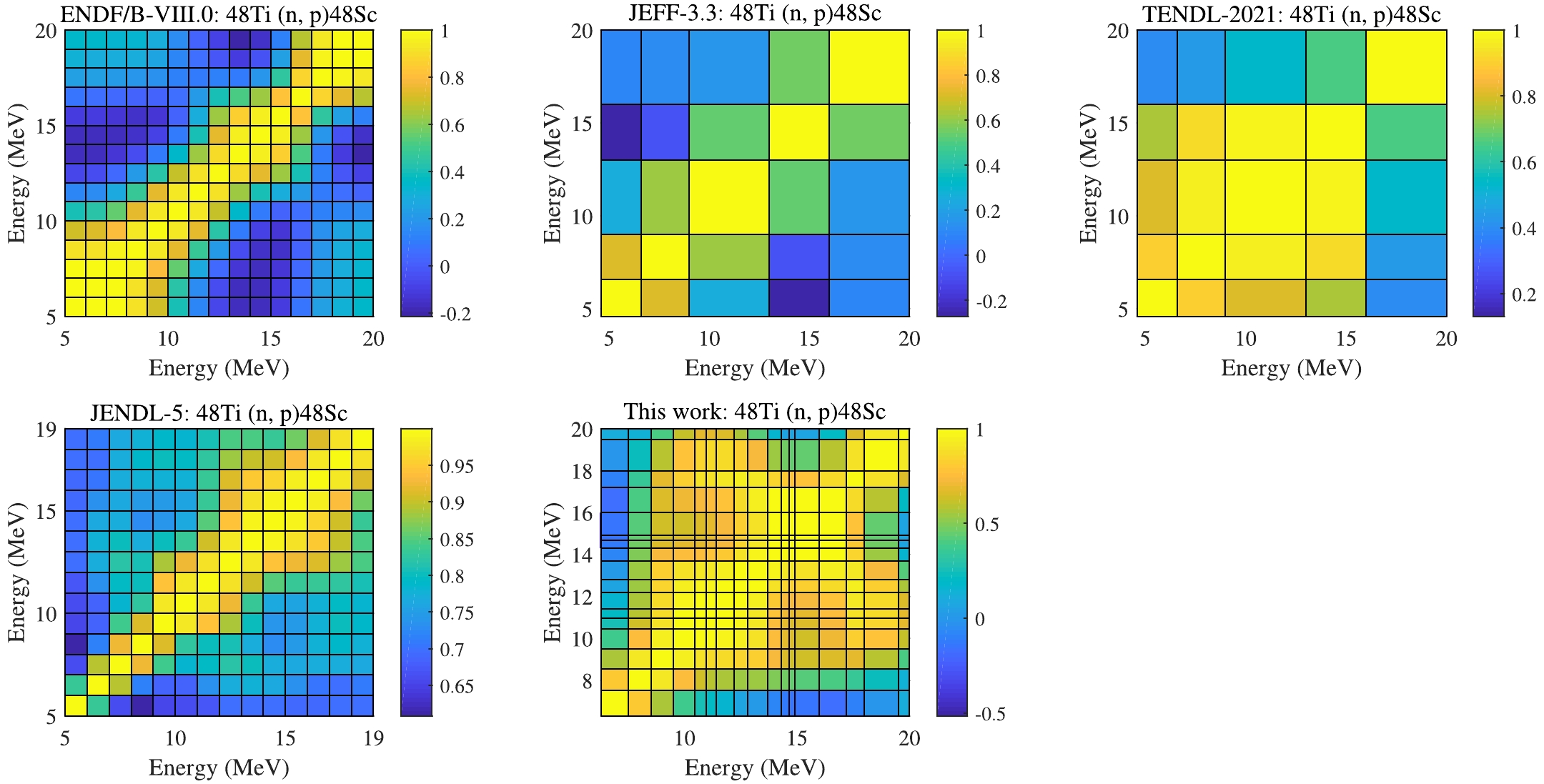
Figure 14. (color online) Comparison of the correlation coefficient matrices for (n, p) in ENDF/B-VIII.0, JEFF-3.3, TENDL-2021, JENDL-5 and this work.
-
For scarce of measurements, two sets of experimental data of natural Ti are selected in this reaction. The input RUs of these measurements are about 6% − 8%, which are shown in Fig. 15, and our derived uncertainties can also cover the other evaluations and experimental data successfully in Fig. 15. Meanwhile, it deserves to mention that CM evaluations in ENDF/B-VIII.0, JENDL-5 and the current UMC-B are more refined than the data in TENDL-2021 and JEFF-3.3 as shown in Fig. 16.
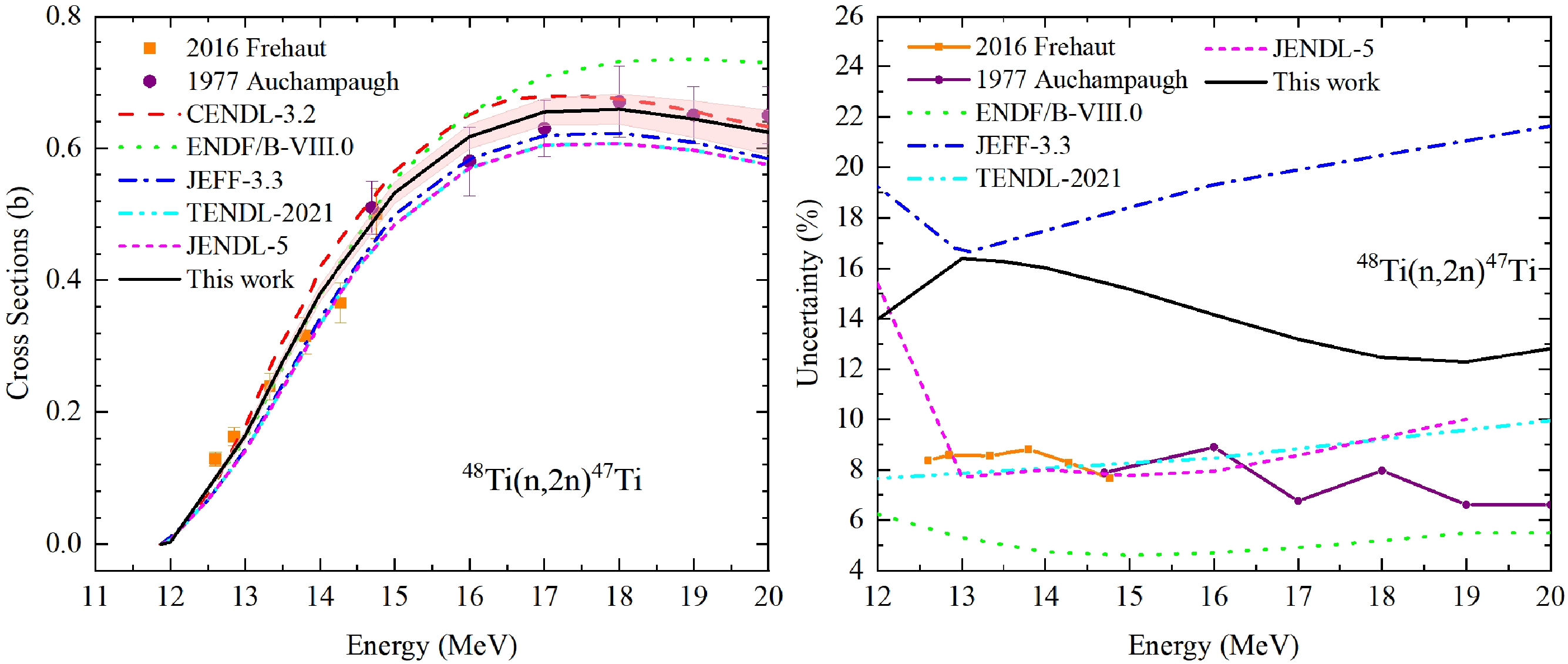
Figure 15. (color online) Comparisons of (n, 2n) cross sections and uncertainties with the evaluations in CENDL-3.2, ENDF/B-VIII.0, JEFF-3.3, TENDL-2021, JENDL-5, this evaluation and the experiment data.
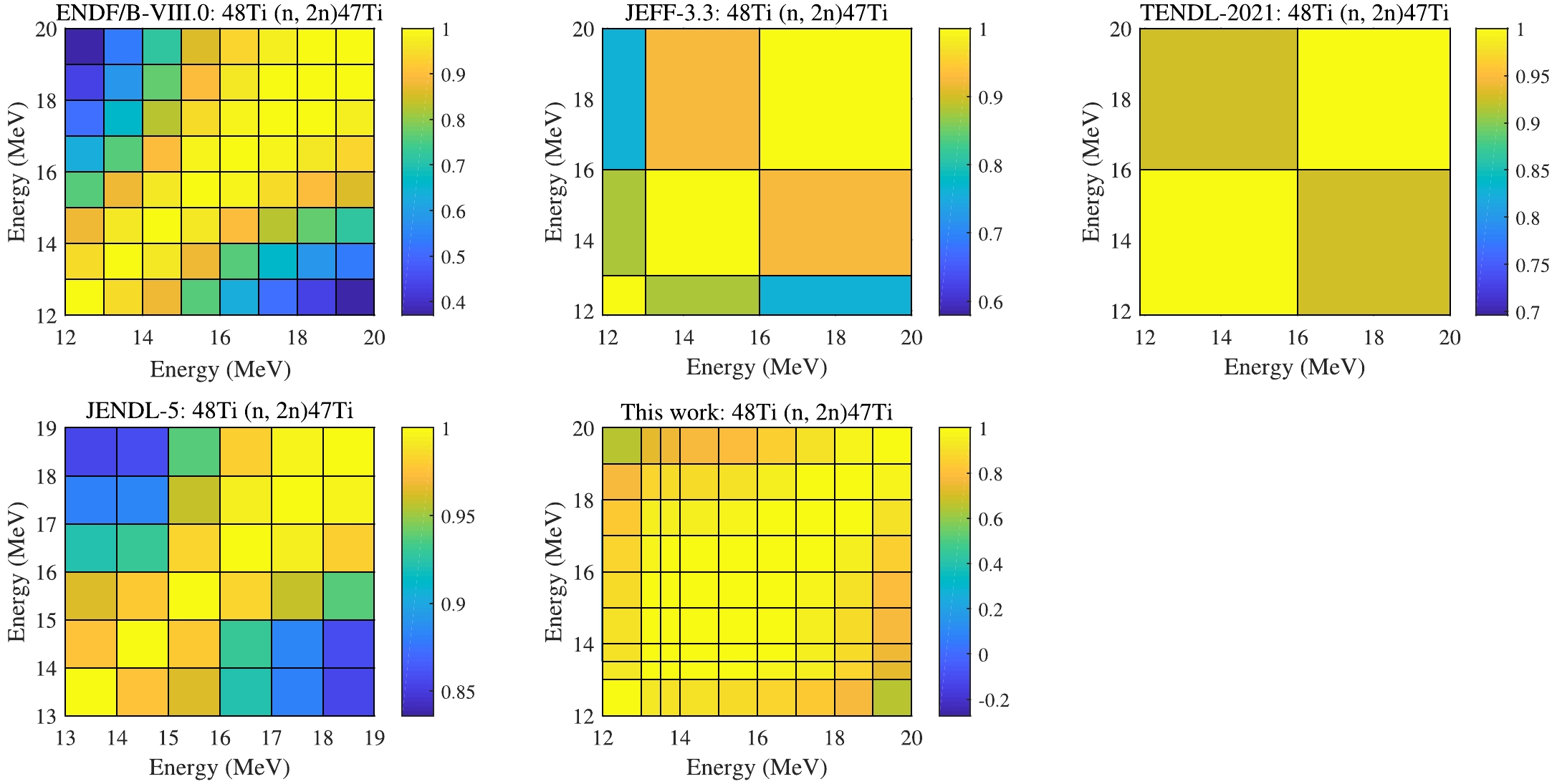
Figure 16. (color online) Comparison of the correlation coefficient matrices for (n, 2n) in ENDF/B-VIII.0, JEFF-3.3, TENDL-2021, JENDL-5 and this work.
-
There is no measurement available for (n, d). Covariance matrices are produced consistently with the data of other reactions. (n, d) are taken as an example in Figs. 17−18 to show the results. The derived RU are reasonable and relative lower than other evaluations in Fig. 17, and CC values looks better predicted by UMC-B and KALMAN in JENDL-5 than others in Fig. 18.
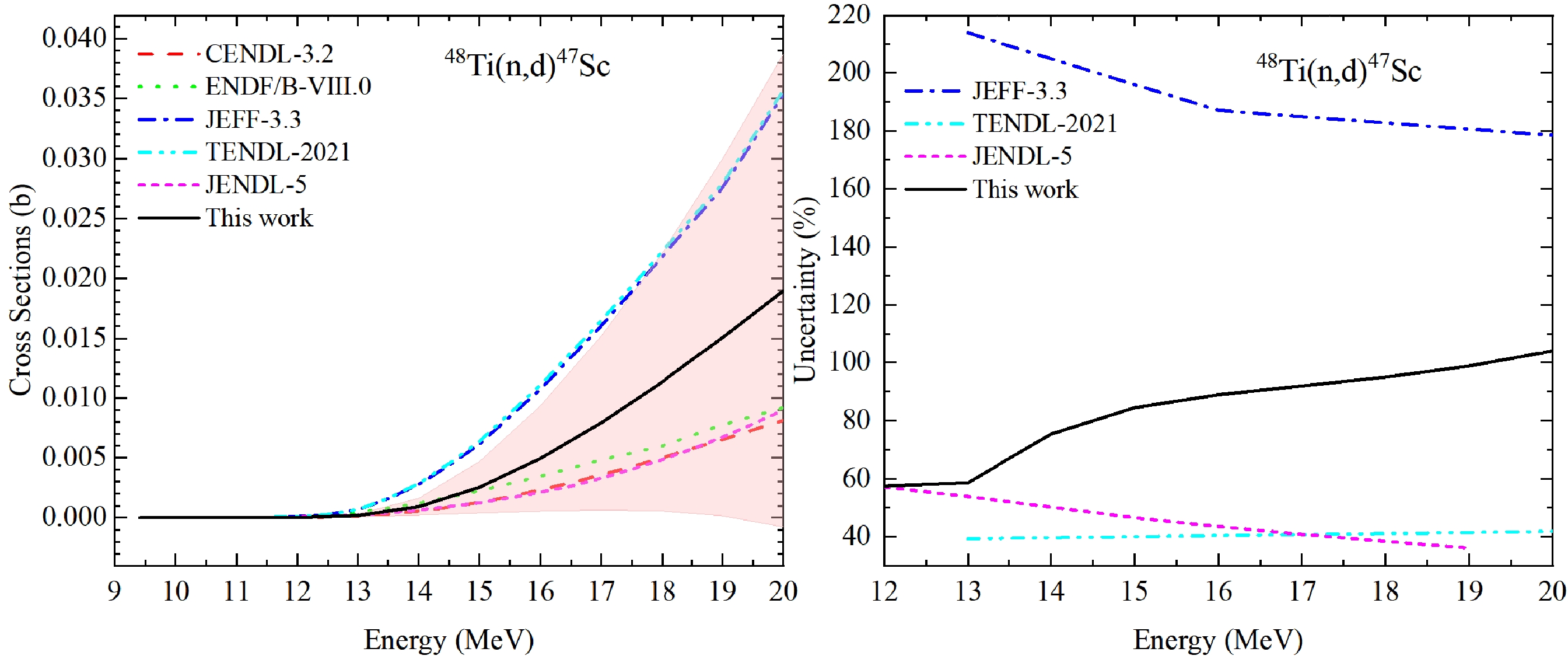
Figure 17. (color online) Comparisons of (n, d) cross sections and uncertainties with the evaluations in CENDL-3.2, ENDF/B-VIII.0, JEFF-3.3, TENDL-2021, JENDL-5, this evaluation and the experiment data.
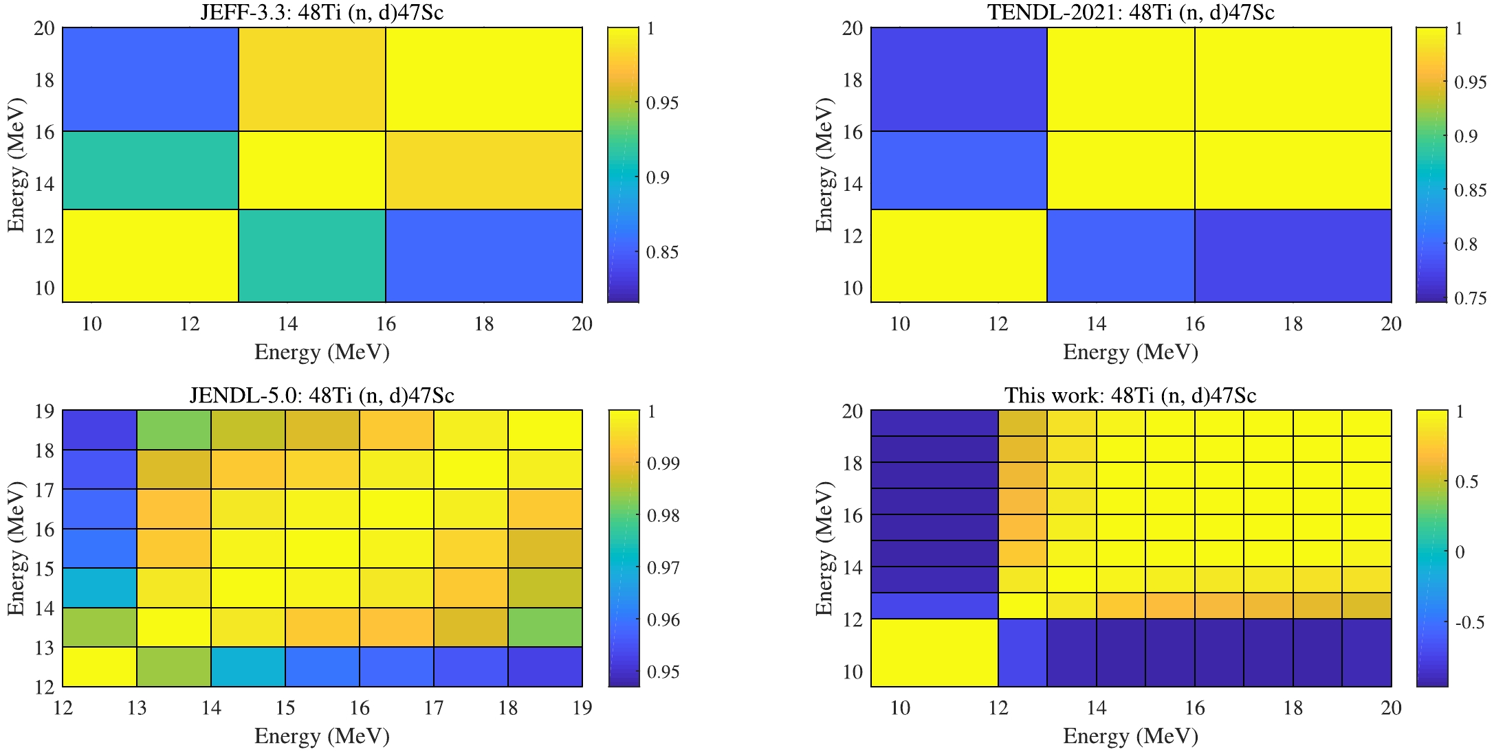
Figure 18. (color online) Comparison of the correlation coefficient matrices for (n, d) in JEFF-3.3, TENDL-2021, JENDL-5 and this work.
-
In this work, covariance matrices of eight main neutron and charged particle emission reactions from n+48Ti in the fast neutron energy region below 20 MeV are calculated by UMC-B method. Cholesky decomposition method is used to realize the correlation sampling of 19 model parameters in the calculation. The current results are compared with the evaluations in CENDL-3.2, ENDF/B-VIII.0, JEFF-3.3, TENDL-2021 and JENDL-5. Satisfying calculations and uncertainty estimates are obtained based on the current preliminary analysis of the experimental data.
In the future, further development of the framework and computational techniques will be carried out to make UMC-B more feasible to a wider range of nuclide systems.
-
The authors are also grateful to the kind discussions with Prof. A.J. Koning from IAEA, Prof. Xubo Ma from North China Electric Power University and Prof. Zehua Hu from Institute of Applied Physics and Computational Mathematics.
Evaluation of neutron cross sections of 48Ti based on the Unified-Monte-Carlo-B method
- Received Date: 2024-03-19
- Available Online: 2024-07-15
Abstract: A cross section evaluation of neutron induced reactions on 48Ti is undertaken using the Unified Monte Carlo-B (UMC-B) approach. The evaluation concentrates on estimating the covariance and the use of the UMC-B allows avoiding the deficiencies of linear regression brought by the traditional least squares method. Eight main neutron and charged particle emission reactions from n+48Ti in the fast neutron energy region below 20 MeV are studied in this work. The posterior probability density function (PDF) of each neutron cross section is obtained in a UMC-B Bayesian approach by convoluting the model PDFs sampled based on model parameters and the likelihood functions for the experimental data. Nineteen model parameters including level density, pair corrections, optical model and Kalbach matrix element parameter are stochastically sampled with the assumption of normal distributions to estimate the model uncertainty. The Cholesky factorization approach is applied to consider potential parameter correlations. Finally, the posterior covariance matrices are generated using the UMC-B generated weights. The new evaluated results are compared with the CENDL-3.2, ENDF/B-VIII.0, JEFF-3.3, TENDL-2021 and JENDL-5 evaluations and differences are discussed.


 DownLoad: