


 Abstract
 HTML
HTML Reference
 Related
 PDF
PDF


-
The universe is expanding at an accelerating rate, which is in contrast with the deceleration predicted by the standard Friedmann model. This observation, based on data of supernovae [1, 2] and cosmic microwave background (CMB) radiation [3, 4], has generated significant interest in alternative theories of gravity. One such theory is massive gravity, which involves assigning a mass to the graviton. This modification allows for a description of our universe's accelerating expansion without the need for a cosmological constant. In the framework of modern particle physics, the gravitational field can be understood as a theory of a spin-2 graviton [5, 6]. The concept of massive gravity dates back to 1939 when Fierz and Pauli constructed a linear theory of massive gravity [7]. However, this theory suffers from a problem known as the Boulware-Deser ghost at the nonlinear level [8, 9]. In recent years, a ghost-free massive theory, known as de Rham-Gabadadze-Tolley (dGRT) massive gravity [10–12], was proposed, addressing the ghost issue. In dGRT gravity theory, researchers have investigated a class of charged black holes and their thermodynamics in asymptotically AdS space-time [13, 14]. The coefficients in the potential associated with the graviton mass have been found to play a similar role to the charge in thermodynamic phase space. Other black hole solutions have also been studied within the framework of massive gravity [15–24].
In the low-energy limit of string theory, Einstein's gravity is recovered along with a non-minimal scalar dilaton field coupled to axions and gauge fields [25]. In the context of coupling gravity to other gauge fields, the dilaton field is indispensable and plays a fundamental role in string theory. Its presence is necessary for the consistency of the theory. Moreover, the dilaton field has a significant impact on the causal structure of black holes; it induces modifications that result in curvature singularities occurring at finite radii [26–32]. There is evidence that the dilaton potential, which is a generalization of the cosmological constant, modifies the asymptotic behavior of solutions, making them neither flat nor (A)dS [33–37]. Furthermore, exploring the coupling of the dilaton field to construct a unified theory of all interactions leads to scalar-tensor type generalizations of general relativity. These generalizations involve incorporating different types of curvature corrections into the standard Einstein-Hilbert Lagrangian coupled to the scalar field [38−40]. One particular model that has received significant attention is Einstein-dilaton-Gauss-Bonnet (EdGB) gravity [41, 42], which incorporates a coupling function. Dilaton charges in this model are expressed as black hole masses, with a scalar dilaton field acting as a secondary hair. Black holes in various dimensions have been extensively studied within the framework of EdGB gravity [43−47].
Recently, a scalar extension of dRGT massive gravity, known as massive Einstein-dilaton gravity [48], was explored. This extension considers the coupling of the dilaton field to the terms of the massive graviton. Additionally, a specific class of static and spherically symmetric solutions for dilatonic black holes has been investigated. Building upon these recent advancements, our objective is to go beyond them and obtain the solutions for charged black holes in Maxwell-dilaton-massive gravity. In particular, we highlight the following points of focus. (i) The constructed Lagrangians consider the non-minimal coupling of the dilaton field solely to the terms of the graviton, as indicated in Eq. (1). It is suggested that the coupling to the Maxwell field is minimal. (ii) In contrast to Ref. [48], we maintain an equal coupling strength for each term of the graviton unless otherwise specified for simplification. (iii) Utilizing the derived Lagrangians, our aim is to obtain solutions for charged black holes within the framework of Maxwell-dilaton-massive gravity. Subsequently, we investigate the properties of these novel solutions and explore their unique characteristics.
The paper is organized as follows. In Sec. II, we present the charged black hole solutions in four dimensional Maxwell-dilaton-massive gravity. In Sec. III, we further discuss the thermodynamic properties of these black holes in canonical and grand canonical ensembles. Finally, a brief discussion is presented in Sec. IV.
-
By considering the nonminimal couplings of the dilaton field φ to the graviton, the action for Maxwell-dilaton-massive gravity can be expressed in four dimensional space-time as
$ I=\frac{1}{16 \pi} \int {\rm d}^{4} x \sqrt{-g} \left({\cal{R}}-F_{\mu\nu} F^{\mu\nu} -2(\nabla \varphi)^2-V(\varphi) + {\rm e}^{-2\beta \varphi}{\cal{L}}_m\right), $

(1) where
$ V(\varphi) $ is a potential for the dilaton field φ, and$ F_{\mu\nu} $ is the electromagnetic field tensor. The exponential factor of the last term in Eq. (1) denotes the nonminimal coupling of the scalar dilaton field to the massive graviton with coupling constant β, and$ {\cal{L}}_m $ is the so-called graviton action [10, 11]$ {\cal{L}}_m= m_0^2 \sum\limits_{i=1}^{4} \eta_i {\cal{U}}_i(g,h), $

(2) where
$ m_0 $ is the mass of the graviton, and$ \eta_i $ are the dimensionless parameters used to distinguish different contributions of$ {\cal{U}}_i $ . Moreover, h is a fixed rank-2 symmetric tensor, and$ {\cal{U}}_i $ satisfies the following recursion relation:$ \begin{aligned}[b]& {\cal{U}}_1 = [K]=K^{\mu}_{\mu}, \\ & {\cal{U}}_2 = [K]^2 - [K^2], \\ & {\cal{U}}_3 = [K]^3 - 3[K][K^2] + 2[K^3],\\ & {\cal{U}}_4 = [K]^4 - 6[K^2][K]^2 + 8[K^3][K] + 3[K^2]^2 - 6[K^4]. \end{aligned} $

(3) Here,
$ K^{\mu}_{\nu}=\sqrt{g^{\mu\tau}h_{\tau\nu}} $ .Generally, the equations of motion can be obtained by computing the variation in action with respect to the field variables
$ g_{\mu\nu} $ , φ, and$ A_{\mu} $ as$ \begin{aligned}[b] G_{\mu\nu} =\;&{\cal{R}}_{\mu\nu}-\frac{1}{2}{\cal{R}} g_{\mu\nu}\\ =\;& 2\partial_{\mu}\varphi\partial_{\nu}\varphi -\frac{1}{2}(V + 2\partial^{\tau}\varphi\partial_{\tau}\varphi)g_{\mu\nu}\\&+2(F_{\mu\tau}F_{\nu}^{\tau}-\frac{1}{4}F^2 g_{\mu\nu}) +m_0^2 e^{-2\beta \varphi} \chi_{\mu\nu}, \end{aligned} $

(4) $ \nabla^2\varphi = \frac{1}{4}\big[\frac{\partial V}{\partial \varphi} +2\beta e^{-2\beta \varphi}{\cal{L}}_m \big], $

(5) $ \nabla_\mu F^{\mu\nu} =0, $

(6) where
$ \begin{aligned}[b] \chi_{\mu\nu} =\;& \frac{{\eta}_1}{2}({\cal{U}}_1 g_{\mu\nu}-K_{\mu\nu}) +\frac{{\eta}_2}{2}({\cal{U}}_2 g_{\mu\nu}-2{\cal{U}}_1 K_{\mu\nu} +2K^2_{\mu\nu})\\ & + \frac{{\eta}_3}{2}({\cal{U}}_3 g_{\mu\nu}-3{\cal{U}}_2 K_{\mu\nu} +6{\cal{U}}_1 K^2_{\mu\nu}-6K^3_{\mu\nu}) \\ & + \frac{{\eta}_4}{2}({\cal{U}}_4 g_{\mu\nu}-4{\cal{U}}_3 K_{\mu\nu} +12{\cal{U}}_2 K^2_{\mu\nu}-24{\cal{U}}_1 K^3_{\mu\nu} +24K^4_{\mu\nu}). \end{aligned} $

(7) The metric ansatz for a static spherically symmetric black hole solution takes the form
$ {\rm d}s^2 = -f(r) {\rm d}t^2 +f^{-1}(r) {\rm d}r^2+ r^2R^2(r) {\rm d}\Omega^2,$

(8) where
$ f(r) $ and$ R(r) $ are functions of r, and${\rm d}\Omega^2= {\rm d}\theta^2+ \sin^2\theta {\rm d}\phi^2$ denotes the line element for the two dimensional spherical subspace.Having supposed that the electromagnetic field has a component where only
$ A=A_t(r){\rm d}t $ for the static spherical symmetric metric, we can solve the Maxwell equation (Eq. (6)) as$ F_{rt}=\frac{Q}{r^2 R^2}, $

(9) where Q is the electric charge, making use of Gauss's law,
$Q=\dfrac{1}{4 \pi}\int {^*}F {\rm d}\Omega$ .Distinguished from the dynamical physical metric
$ g_{\mu\nu} $ , the reference metric$ h_{\mu\nu} $ is usually fixed and assumed to be non-dynamical in massive theory. Therefore, we choose the reference metric to be [13−15]$ h_{\mu\nu}= {\rm diag}(0,~ 0,~ c_0^2,~ c_0^2\sin^2\theta), $

(10) where
$ c_0 $ is a positive parameter. From the ansatz (10), the interaction potential in Eq. (3) changes into$ {\cal{U}}_1=\frac{2}{R r},\ \ \ {\cal{U}}_2=\frac{2}{R^2 r^{2}},\ \ \ {\cal{U}}_3={\cal{U}}_4=0. $

(11) $ \chi^{\mu}_{\; \nu} $ in Eq. (7) can be written as$ \chi^1_{\; 1} = \chi^2_{\; 2} = \frac{{\rm e}^{-2\beta \phi}( \eta_1 r R + \eta_2 c_0^2 )}{(r R)^2 },\ \ \ \chi^3_{\; 3} = \chi^4_{\; 4} = \frac{\eta_1 {\rm e}^{-2\beta \phi }}{2 r R }, $

(12) and the components of the equation of motion (4) become
$ \begin{aligned}[b] G^1_{\; 1} =\;& \frac{1}{(r R)^2}[r R (r R)'f'+2r R (r R)'' f+(r R)'^2 f-1] \\=\;&-\frac{V(\varphi)}{2}-f \varphi'^2-\frac{Q^2}{r^4 R^4}+m_0^2 \chi^1_{\; 1} , \end{aligned} $

(13) $\begin{aligned}[b] G^2_{\; 2} =\;& \frac{1}{(r R)^2}[r R (r R)'f'+(r R)'^2 f -1 ]\\=\;&-\frac{V(\varphi)}{2}+f \varphi'^2-\frac{Q^2}{r^4 R^4}+m_0^2 \chi^2_{\; 2} , \end{aligned} $

(14) $\begin{aligned}[b] G^3_{\; 3} =\;& G^4_4=\frac{1}{ 2 r R}[(r R) f'' + 2 (r R)' f'+ 2 (r R)'' f]\\=\;&-\frac{V(\varphi)}{2}-f \varphi'^2+\frac{Q^2}{r^4 R^4}+m_0^2 \chi^3_{\; 3},\end{aligned} $

(15) where the prime ′ denotes differentiation with respect to r.
Calculating
$ G^1_{\; 1}-G^2_{\; 2} $ , we obtain$ \frac{(r R)'' }{r R}=-\varphi'^2, $

(16) which leads to
$ \frac{{\rm d}^2}{{\rm d}r^2}\ln R +\frac{2}{r}\frac{\rm d}{{\rm d}r}\ln R +\left(\frac{\rm d}{{\rm d}r}\ln R\right)^2=-\varphi'^2. $

(17) To obtain the dilaton field φ, it is posited that
$ R(r) $ may be an exponential function of$ \varphi(r) $ $ R(r)={\rm e}^{\alpha \varphi}, $

(18) and Eq. (17) reduces to
$ \alpha \phi '' (r)+\left(\alpha ^2+1\right) \phi '(r)^2+\frac{2 \alpha \phi '(r)}{r}=0,$

(19) where α is a positive constant. Then, the dilaton field can be obtained as
$ \varphi (r) = \frac{\alpha}{1+\alpha^2} \ln\frac{\delta}{r}. $

(20) Here, δ is a constant parameter.
Regarding these solutions together with the electromagnetic field tensor Eq. (9), we can obtain
$ A_t(r)= \left\{ \begin{array}{*{20}{l}} { \dfrac{(\alpha ^2+1) Q} {\alpha ^2-1}\delta ^{-{2 \alpha ^2}/{(\alpha ^2+1})} r^{(-{1-\alpha ^2)}/({1+\alpha ^2})}, }&{\alpha\neq 1}\\{\dfrac{Q \log (r)}{\delta },} & {\alpha =1 } \end{array} \right. $

(21) Note that the potential function
$ A_{t}(r) $ should be vanishing at infinity to be physically reasonable [35]; therefore, the condition$ \alpha<1 $ must be fulfilled, and the solution of$ A_{t}(r) $ is only the first branch in Eq. (21).According to the metric ansatz (8) and expressions for the dilaton field (18) and (20), the Klein-Gordon Eq. (5) becomes
$ \begin{aligned}[b]&\frac{f'}{\alpha ^2+1}+\frac{\left(1-\alpha ^2\right) f}{(\alpha ^2 +1)^2 r} +\frac{ r}{4 \alpha }\frac{\partial V}{\partial \varphi} \\&\quad +\frac{ m_0^2\beta c_0 {\rm e}^{-2\beta \varphi}}{\alpha \delta} \left(\eta_1 \delta {\rm e}^{-\alpha \varphi}+\eta_2 c_0 {\rm e}^{\frac{1-\alpha^2}{\alpha} \varphi} \right)=0. \end{aligned} $

(22) Moreover, we further consider the trace of the gravitational Eq. (4),
$ \begin{align} f'' & +\frac{4( r R)'f'}{rR}+\frac{ 2 f\left((r R')^2+2 r R \left(r R'' +3 R'\right)+R^2+(r R)^2\varphi '^2 \right)}{(r R)^2}\\ & +2 V(\varphi)-\frac{2}{(r R)^2}-m_0^2\sum\limits^4_{i=1}\chi_i^i=0. \end{align} $

(23) Based on the
$ G^3_{\; 3} $ component of the gravitational Eq. (15), Eq. (23) can be written as$ \begin{aligned}[b]& -\frac{f'}{\alpha ^2+1} +\frac{\left(\alpha ^2-1\right) f}{\left(\alpha ^2+1\right)^2 r} -\frac{ r V(\varphi)}{2} +\frac{{\rm e}^{\frac{1-\alpha^2}{\alpha}\varphi } }{\delta} -\frac{ Q^2}{\delta^3} {\rm e}^{\frac{3- \alpha ^2}{\alpha}\varphi}\\&\quad + \frac{m_0^2 c_0 {\rm e}^{-2\beta \varphi}}{\delta}\left(\eta_1 \delta {\rm e}^{-\alpha\varphi } +\eta_2 c_0{\rm e}^{\frac{1-\alpha^2}{\alpha} \varphi}\right) =0 \end{aligned} $

(24) together with the expressions for the dilaton field (20).
Considering Eqs. (22) and (24), we can obtain a first order differential equation for the dilaton field potential,
$ \begin{aligned}[b]&\frac{ \partial V(\varphi )}{\partial \varphi }-2 \alpha V(\varphi ) +\frac{4 \alpha {\rm e}^{\frac{2 \varphi }{\alpha }}}{\delta ^2} -\frac{4 \alpha Q^2 {\rm e}^{\frac{4 \varphi }{\alpha }}}{\delta ^4}\\&\quad +\frac{4 \eta_1 c_0 m_0^2 (\alpha +\beta ) {\rm e}^{-2 \varphi \left(\beta -\frac{1}{2 \alpha }\right)}}{\delta } +\frac{4 \eta_2 c_0^2 m_0^2 (\alpha +\beta ) {\rm e}^{-2 \varphi \left(\beta -\frac{1}{\alpha }\right)}}{\delta ^2} =0, \end{aligned} $

(25) which leads to
$\begin{aligned}[b] V(\varphi)= \;& \frac{2 \alpha ^2 {\rm e}^{\frac{2 \varphi }{\alpha }}}{\left(\alpha ^2-1\right) \delta ^2} +2 \Lambda {\rm e}^{2 \alpha \varphi } -\frac{2 \alpha ^2 Q^2 {\rm e}^{\frac{4 \varphi }{\alpha }}}{\left(\alpha ^2-2\right) \delta ^4} \\& +\frac{4 \alpha c_0 \eta_1 m_0^2 (\alpha +\beta ) {\rm e}^{\varphi \left(\frac{1}{\alpha }-2 \beta \right)}}{\delta \left(2 \alpha ^2+2 \alpha \beta -1\right)}\\ & +\frac{2 \alpha c_0^2 \eta_2 m_0^2 (\alpha +\beta ) {\rm e}^{2 \varphi \left(\frac{1}{\alpha }-\beta \right)}}{\delta ^2 \left(\alpha ^2+\alpha \beta -1\right)}. \end{aligned} $

(26) Here, the last two terms are associated with the coupling between the dilaton field and the graviton, and Λ is a free parameter that is considered to play the role of the cosmological constant, because in the absence of the dilaton field (
$ \alpha=0 $ ), we have$ V=2\Lambda $ , i.e.,$ \Lambda=-\dfrac{d(d-1)}{2l^2} $ , in which l is the radius of the$ (d+1)- $ dimensional AdS spacetime. Then, the metric function$ f(r) $ from Eq. (22) can be also obtained as$ \begin{aligned}[b]&f(r)= \; -m r^{\frac{\alpha ^2-1}{\alpha ^2+1}} -\frac{\left(\alpha ^2+1\right) \left(\dfrac{\delta }{r}\right)^{-\frac{2 \alpha ^2}{\alpha ^2+1}}}{\alpha ^2-1} \\&+\frac{2 \left(\alpha ^2+1\right)^2 Q^2 \delta ^{-\frac{4 \alpha ^2}{\alpha ^2+1}} r^{\frac{2 \left(\alpha ^2-1\right)}{\alpha ^2+1}}}{\alpha ^4-3 \alpha ^2+2} \\&+\frac{\left(\alpha ^2+1\right)^2 \Lambda \delta ^{\frac{2 \alpha ^2}{\alpha ^2+1}} r^{\frac{2}{\alpha ^2+1}}}{\alpha ^2-3}\\&\quad -\frac{\left(\alpha ^2+1\right)^2 c_0 \eta_1 m_0^2 \delta ^{-\frac{\alpha (\alpha +2 \beta )}{\alpha ^2+1}} r^{\frac{2 \alpha ^2+2 \alpha \beta +1}{\alpha ^2+1}}}{\left(\alpha ^2+2 \alpha \beta +2\right) \left(2 \alpha ^2+2 \alpha \beta -1\right)} \\& \quad -\frac{\left(\alpha ^2+1\right)^2 c_0^2 \eta_2 m_0^2 \left(\dfrac{\delta }{r}\right)^{-\frac{2 \alpha (\alpha +\beta )}{\alpha ^2+1}}}{\left(\alpha ^2+\alpha \beta -1\right) \left(\alpha ^2+2 \alpha \beta +1\right)} \end{aligned} $

(27) where m is an integration constant related to the mass of the black hole, as shown below. In the absence of the dilaton field
$ (\alpha=0) $ , the metric function$ f(r) $ becomes$ f(r)=1-\frac{m}{r}+\frac{ Q^2 }{ r^{2}}+\frac{1}{2} \eta_1m_0^2 r+\eta_2 m_0^2-\frac{1}{3} \Lambda r^2, $

(28) as presented in Ref. [14] (the value of Q as
$ \alpha\rightarrow0 $ is half of that in Ref. [14] owing to the different factors of the electromagnetic action$ F^2 $ ). Here, we set$ c_0=1 $ . Obviously, the metric function$ f(r) $ does not describe an AdS space unless$ m_0=0 $ .At infinity, the dominant term of the solution
$ f(r) $ approaches$ \begin{aligned}[b] \lim\limits_{r\to \infty} f(r)= \;& \frac{\left(\alpha ^2+1\right)^2 \Lambda \delta ^{\frac{2 \alpha ^2}{\alpha ^2+1}} r^{\frac{2}{\alpha ^2+1}}}{\alpha ^2-3} \\& -\frac{\left(\alpha ^2+1\right)^2 c_0 \eta_1 m_0^2 \delta ^{-\frac{\alpha (\alpha +2 \beta )}{\alpha ^2+1}} r^{\frac{2 \alpha ^2+2 \alpha \beta +1}{\alpha ^2+1}}}{\left(\alpha ^2+2 \alpha \beta +2\right) \left(2 \alpha ^2+2 \alpha \beta -1\right)} \end{aligned}$

(29) For example, taking
$ \alpha =\beta=0.6 $ , we have$ \lim\limits_{r\to \infty} f(r)=-1.36482 m_0^2 c_0 \eta_1 r^{1.79412}- 0.700606 \Lambda r^{1.47059}, $

(30) where we set
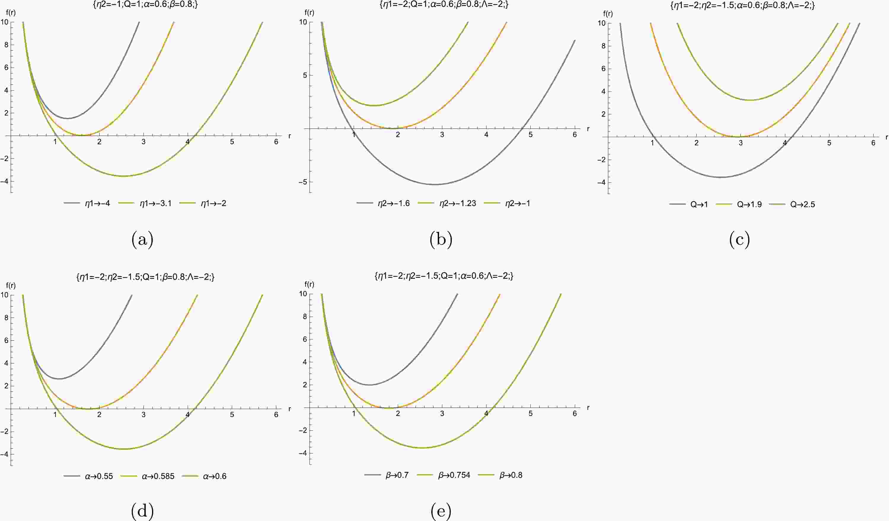
$ \delta=1 $ for simplicity. Clearly, the metric function is neither asymptotically flat nor asymptotically (A)dS. To comprehensively understand the behavior of the metric function, we graphically present the dependence of the function$ f(r) $ . Plots of metric function versus r are shown in Fig. 1 in terms of different parameters, which show that two horizons and extreme and naked singularity black holes can occur by choosing proper parameters.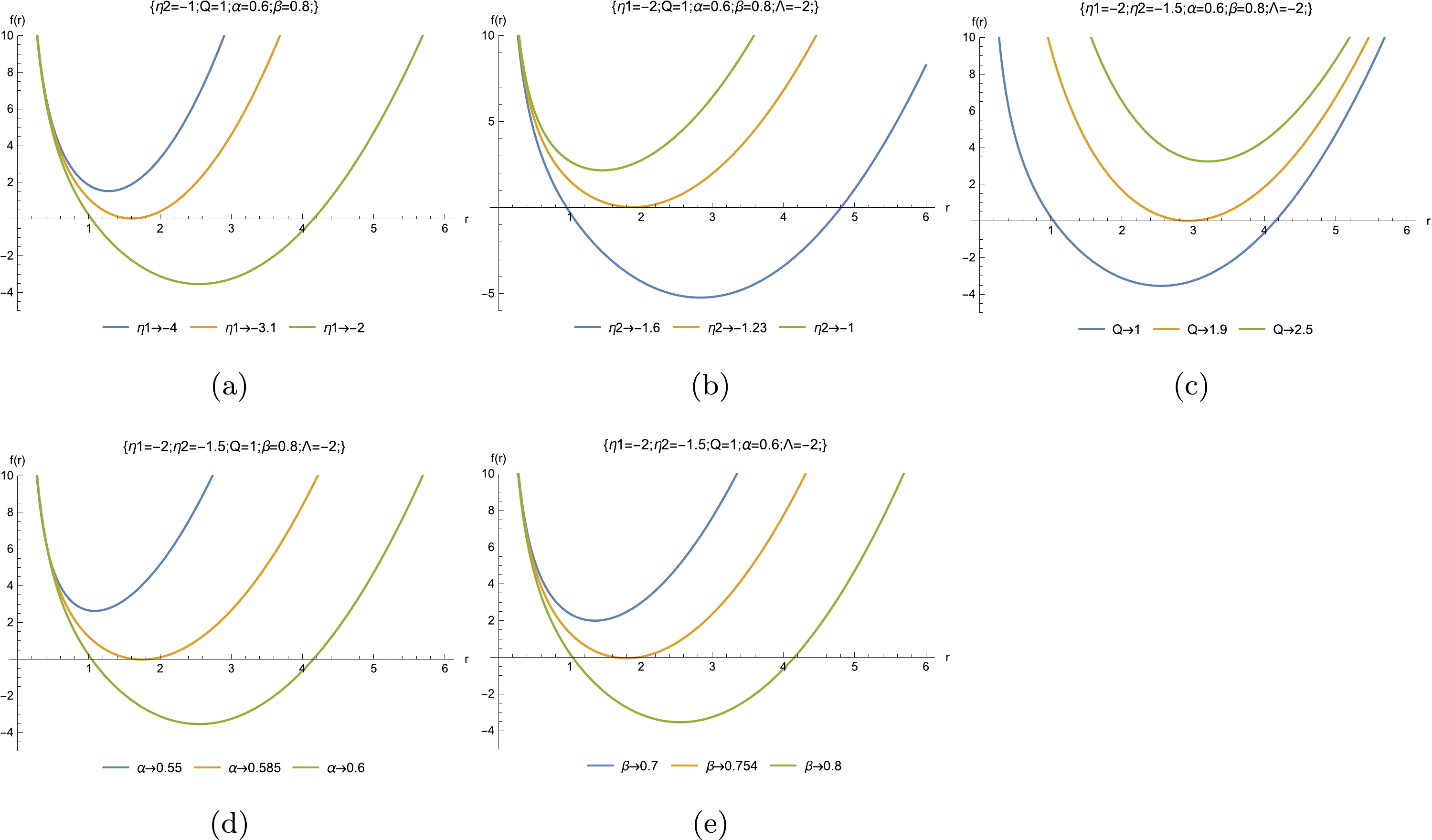
Figure 1. (color online) Diagrams of metric function
$ f(r) $ versus r for$ m_0=c_0=\delta=m=1 $ , and$ \Lambda=-2 $ .Now, we consider spacetime singularities and calculate the Kretschmann scalar
$ \begin{aligned}[b] {\cal{R}}^{\mu\nu\rho\sigma} {\cal{R}}_{\mu\nu\rho\sigma} = & f \left(\frac{8 f' (r R)' (r R)'' }{(r R)^2}-\frac{8 \left((r R)'\right)^2}{(r R)^4}\right)+\frac{4 {f'}^2 \left((r R)'\right)^2}{(r R)^2}\\ & +\frac{4 f^2 \left(\left((r R)'\right)^4+2 (r R)^2 \left((r R)'' \right)^2\right)}{(r R)^4}+\frac{4}{(r R)^4}+{f''} ^2. \end{aligned} $

(31) Evidently, the Kretschmann scalar is not singular at the horizons. These points are simply singularities of coordinates as for a black hole. From the leading terms of the asymptotic behaviors of the metric at the origin, we have
$ \lim\limits_{r\rightarrow0} {\cal{R}}^{\mu\nu\rho\sigma}{\cal{R}}_{\mu\nu\rho\sigma}=\infty,\ \ \lim\limits_{r\rightarrow \infty} {\cal{R}}^{\mu\nu\rho\sigma}{\cal{R}}_{\mu\nu\rho\sigma}=0, $

(32) where the Kretschmann scalar
$ {\cal{R}}^{\mu\nu\rho\sigma}{\cal{R}}_{\mu\nu\rho\sigma} $ is divergent at origin$ r=0 $ , finite for$ r>0 $ , and vanishes at infinity, which suggests the origin$ r=0 $ is an essential and physical singularity in the spacetime. -
In this section, we discuss the thermodynamic properties of black holes from the previous section. The black hole entropy can be defined using the well-established Wald's approach [49, 50]:
$ S=-2\pi \int_{\Sigma} {\rm d}^{d-2}x \sqrt{\sigma}\frac{\partial {\cal{L}}}{\partial{\cal{R}}_{\mu\nu\kappa\lambda}}\varepsilon_{\mu\nu}\varepsilon_{\kappa\lambda}, $

(33) where Σ denotes a Killing horizon with binormal
$ \varepsilon_{\mu\nu} $ , σ is the determinant of the induced metric on the horizon surface, and$ {\cal{L}} $ is the gravitational Lagrangian. Therefore, the entropy of these black holes is$ S=\pi \delta ^{\frac{2 \alpha ^2}{\alpha ^2+1}} r_h^{\frac{2}{\alpha ^2+1}}.$

(34) This is identified with the so-called entropy-area law. Refs. [14–16, 51, 52] show that graviton mass has only a small effect on the form of entropy and is just a correction for the horizon radius.
Moreover, the temperature of black holes in terms of the null Killing vector
$ (\dfrac{\partial}{\partial t})^a $ at the horizon reads as$ \begin{aligned}[b] T =\; &\frac{\kappa}{2 \pi}=\frac{1}{4 \pi}\frac{\partial f(r)}{\partial r}\big|_{r=r_h} =\frac{\left(\alpha ^2+1\right) Q^2 \delta ^{-\frac{4 \alpha ^2}{\alpha ^2+1}} r_h^{\frac{\alpha ^2-3}{\alpha ^2+1}}}{2 \pi \left(\alpha ^2-2\right)} \\& -\frac{\left(\alpha ^2+1\right) \Lambda \delta ^{\frac{2 \alpha ^2}{\alpha ^2+1}} r_h^{\frac{2}{\alpha ^2+1}-1}}{4 \pi } -\frac{\left(\alpha ^2+1\right) \left(\dfrac{\delta }{r_h}\right){}^{-\frac{2 \alpha ^2}{\alpha ^2+1}}}{4 \pi \left(\alpha ^2-1\right) r_h} \\ &-\frac{\left(\alpha ^2+1\right) c_0 \eta _1 m_0^2 \left(\dfrac{r_h}{\delta }\right){}^{\frac{\alpha (\alpha +2 \beta )}{\alpha ^2+1}}}{4 \pi \left(2 \alpha ^2+2 \alpha \beta -1\right)} \\& -\frac{\left(\alpha ^2+1\right) c_0^2 \eta _2 m_0^2 \left(\dfrac{\delta }{r_h}\right){}^{-\frac{2 \alpha (\alpha +\beta )}{\alpha ^2+1}}}{4 \pi \left(\alpha ^2+\alpha \beta -1\right) r_h} .\end{aligned} $

(35) From the definition of ADM mass [53], we obtain
$ \begin{aligned}[b] M =\; & \frac{\delta^{\frac{2\alpha^2}{1+\alpha^2}}m}{2(1+\alpha^2)} = \frac{\left(\alpha ^2+1\right) Q^2 \delta ^{-\frac{2 \alpha ^2}{\alpha ^2+1}} r_h^{\frac{\alpha ^2-1}{\alpha ^2+1}}}{\alpha ^4-3 \alpha ^2+2}\\ &+\frac{\left(\alpha ^2+1\right) \Lambda \delta ^{\frac{4 \alpha ^2}{\alpha ^2+1}} r_h^{\frac{3-\alpha ^2}{\alpha ^2+1}}}{2 \left(\alpha ^2-3\right)} -\frac{\left(\dfrac{1}{r_h}\right){}^{-\frac{2 \alpha ^2}{\alpha ^2+1}} r_h^{\frac{1-\alpha ^2}{\alpha ^2+1}}}{2 \left(\alpha ^2-1\right)}\\ & -\frac{\left(\alpha ^2+1\right) c_0 \eta _1 m_0^2 \delta ^{\frac{\alpha (\alpha -2 \beta )}{\alpha ^2+1}} r_h^{\frac{\alpha ^2+2 \alpha \beta +2}{\alpha ^2+1}}}{2 \left(\alpha ^2+2 \alpha \beta +2\right) \left(2 \alpha ^2+2 \alpha \beta -1\right)}\\& -\frac{\left(\alpha ^2+1\right) c_0^2 \eta _2 m_0^2 \delta ^{\frac{2 \alpha ^2}{\alpha ^2+1}} r_h^{\frac{1-\alpha ^2}{\alpha ^2+1}} \left(\dfrac{\delta }{r_h}\right){}^{-\frac{2 \alpha (\alpha +\beta )}{\alpha ^2+1}}}{2 \left(\alpha ^2+\alpha \beta -1\right) \left(\alpha ^2+2 \alpha \beta +1\right)}. \end{aligned} $

(36) The electric potential Φ of black holes, measured by an observer located at infinity with respect to the horizon, can be calculated using the following standard relation [38]:
$ \Phi=A_{\mu} Z^{\mu}|_{r\rightarrow \infty}-A_{\mu} Z^{\mu}|_{r=r_h},$

(37) where
$Z=C \partial_t$ is the null generator of the horizon. Therefore, using Eq. (21), the electric potential may be obtained as$ \Phi= -\frac{C (\alpha ^2+1) Q \delta ^{-\frac{2 \alpha ^2}{\alpha ^2+1}} r^{-\frac{1-\alpha ^2}{1+\alpha ^2}}}{\alpha ^2-1}. $

(38) Regarding the parameters S and Q as a complete set of extensive parameters, the Smarr-type mass formula for the new black holes is expressed as
$ \begin{aligned}[b] M(S,Q) =\; & \frac{\left(\alpha ^2+1\right) Q^2 \delta ^{-\alpha ^2} (\frac{S}{\pi})^{\frac{1}{2} \left(\alpha ^2-1\right)}}{\alpha ^4-3 \alpha ^2+2} +\frac{\delta ^{-\alpha ^2} \left(\dfrac{S}{\pi}\right)^{\frac{1}{2} \left(\alpha ^2+1\right)}}{2-2 \alpha ^2} \\&-\frac{\left(\alpha ^2+1\right) c_0 \eta_1 m_0^2 \delta ^{-\alpha (\alpha +2 \beta )} \left(\dfrac{S}{\pi}\right)^{\frac{\alpha ^2}{2}+\alpha \beta +1}}{2 \left(\alpha ^2+2 \alpha \beta +2\right) \left(2 \alpha ^2+2 \alpha \beta -1\right)} \\ & -\frac{\left(\alpha ^2+1\right) c_0^2 \eta_2 m_0^2 \delta ^{-\alpha (\alpha +2 \beta )} \left(\dfrac{S}{\pi}\right)^{\frac{1}{2} \left(\alpha ^2+2 \alpha \beta +1\right)}}{2 \left(\alpha ^2+2 \alpha \beta +1\right) (\alpha (\alpha +\beta )-1)} \\&+\frac{\left(\alpha ^2+1\right) \Lambda \delta ^{\alpha ^2} \left(\dfrac{S}{\pi}\right)^{\frac{3}{2}-\frac{\alpha ^2}{2}}}{2 \left(\alpha ^2-3\right)} \end{aligned} $

(39) We may find that the intensive parameters T and Φ, conjugated to the black hole entropy and charge, satisfy the following relations:
$ T=\left(\frac{\partial M(S,Q)}{\partial S}\right)_Q,\ \ \ \Phi=\left(\frac{\partial M(S,Q)}{\partial Q}\right)_S, $

(40) provided that C is chosen as
$C=\frac{2}{2-\alpha ^2}. $

(41) Note that
$ C= 1 $ and$ \Phi=\dfrac{ Q }{r} $ in the case of$ \alpha=0 $ . The intensive quantities calculated using Eq. (40), regarded as the temperature and electric potential, coincide with Eqs. (35) and (38). Thus, these thermodynamic quantities satisfy the first law of thermodynamics, expressed as$ {\rm d} M = T {\rm d}S + \Phi {\rm d}Q $

(42) Next, we investigate the critical behaviors of charged black holes both in the grand canonical and canonical ensembles and set
$ m_0=c_0=\delta=1 $ and$ \Lambda=-2 $ for simplicity in the following discussions. -
In the grand canonical ensemble with a fixed chemical potential Φ associated with the charge Q, the Gibbs free energy is written as
$ \begin{aligned}[b] G =\; & M-TS-\Phi Q\\ =\;&\frac{r_h}{4}-\frac{1}{8} \left(\alpha ^4-3 \alpha ^2+2\right) \Phi ^2 r_h^{\frac{1-\alpha ^2}{\alpha ^2+1}} \\& +\frac{\left(\alpha ^2-1\right) \left(\alpha ^2+1\right) \Lambda r_h^{\frac{3-\alpha ^2}{\alpha ^2+1}}}{4 \left(\alpha ^2-3\right)}\\ & +\frac{\left(\alpha ^2+1\right) \eta _2 \left(\alpha ^2+2 \alpha \beta -1\right) r_h^{\frac{\alpha ^2+2 \alpha \beta +1}{\alpha ^2+1}}}{4 \left(\alpha ^2+\alpha \beta -1\right) \left(\alpha ^2+2 \alpha \beta +1\right)} \\&+\frac{\alpha \left(\alpha ^2+1\right) \eta _1 (\alpha +2 \beta ) r_h^{\frac{\alpha ^2+2 \alpha \beta +2}{\alpha ^2+1}}}{4 \left(\alpha ^2+2 \alpha \beta +2\right) \left(2 \alpha ^2+2 \alpha \beta -1\right)} \end{aligned} $

(43) The temperature of the black hole is
$ \begin{aligned}[b] T =\; & \frac{\left(\alpha ^2-2\right) \left(\alpha ^2-1\right)^2 \Phi ^2}{8 \pi \left(\alpha ^2+1\right) r_h} -\frac{\left(\alpha ^2+1\right) \Lambda r_h^{\frac{2}{\alpha ^2+1}-1}}{4 \pi } \\&-\frac{\left(\alpha ^2+1\right) r_h^{\frac{\alpha ^2-1}{\alpha ^2+1}}}{4 \pi \left(\alpha ^2-1\right)} -\frac{\left(\alpha ^2+1\right) \eta _1 r_h^{\frac{\alpha (\alpha +2 \beta )}{\alpha ^2+1}}}{4 \pi \left(2 \alpha ^2+2 \alpha \beta -1\right)} \\& -\frac{\left(\alpha ^2+1\right) \eta _2 r_h^{\frac{2 \alpha (\alpha +\beta )}{\alpha ^2+1}-1}}{4 \pi \left(\alpha ^2+\alpha \beta -1\right)} \end{aligned} $

(44) and the corresponding heat capacity is
$ C_\Phi=\frac{-16 \pi ^2 T r^{\frac{2}{\alpha ^2+1}+1}(\alpha ^4-1)^{-1} }{\dfrac{\left(\alpha ^4-3 \alpha ^2+2\right) \Phi ^2}{\alpha ^2+1}+\dfrac{2 \eta _2 \left(\alpha ^2+2 \alpha \beta -1\right) r_h^{\frac{2 \alpha (\alpha +\beta )}{\alpha ^2+1}}}{\left(\alpha ^2-1\right) \left(\alpha ^2+\alpha \beta -1\right)}+\dfrac{2 \alpha \eta _1 (\alpha +2 \beta ) r_h^{\frac{\alpha (\alpha +2 \beta )}{\alpha ^2+1}+1}}{\left(\alpha ^2-1\right) \left(2 \alpha ^2+2 \alpha \beta -1\right)}-2 \Lambda r_h^{\frac{2}{\alpha ^2+1}}+\dfrac{2 r_h^{\frac{2 \alpha ^2}{\alpha ^2+1}}}{\alpha ^2-1}} $

(45) According to Eq. (43), the term
$ \eta_1 $ vanishes for$ \alpha\rightarrow 0 $ , which means that the term$ \eta_2 $ is considerably more important in the case without the dilaton field. However, in the case with the dilaton field, i.e.,$ \alpha\neq 0 $ , considering the asymptotic behaviors of the Gibbs free energy, the term$ \eta_1 $ plays a more important role than$ \eta_2 $ as$ r_h\rightarrow \infty $ .Using the conditions of the inflection point in the van der Waals (VdW) system,
$ \frac{\partial T}{\partial r_h}\left|_{\Phi=\Phi_c,r_h=r_c}\right. =\frac{\partial^2 T}{\partial r_h^2}\left|_{\Phi=\Phi_c,r_h=r_c}\right. =0, $

(46) we can obtain the critical
$ \Phi_c $ and the equation of the critical radius of the black hole as$ \begin{aligned}[b] \Phi^2_{c}=\; &\frac{2 \left(\alpha ^2+1\right)}{\left(\alpha ^2-2\right) \left(\alpha ^2-1\right)^2}\left( \left(\alpha ^2-1\right) \Lambda r_c^{\frac{2}{\alpha ^2+1}}\right. \\& -\frac{\eta_2 \left(\alpha ^2+2 \alpha \beta -1\right) }{\alpha ^2+\alpha \beta -1}\cdot r_c^{\frac{2 \alpha (\alpha +\beta )}{\alpha ^2+1}} \\ & \left. -r_c^{\frac{2 \alpha ^2}{\alpha ^2+1}} -\frac{\alpha \eta_1 (\alpha +2 \beta ) }{2 \alpha ^2+2 \alpha \beta -1}\cdot r_c^{\frac{\alpha (\alpha +2 \beta )}{\alpha ^2+1}+1} \right) \end{aligned} $

(47) $ \begin{aligned}[b] 0=\; & \alpha ^2 +\left(1-\alpha ^2\right) \Lambda r_c^{\frac{2-2 \alpha ^2}{\alpha ^2+1}}\\&+\frac{\alpha \eta _2 (\alpha +\beta ) \left(\alpha ^2+2 \alpha \beta -1\right) }{\alpha ^2+\alpha \beta -1}\cdot r_c^{\frac{2 \alpha \beta }{\alpha ^2+1}} \\ &+\frac{\alpha \eta _1 (\alpha +2 \beta ) \left(2 \alpha ^2+2 \alpha \beta +1\right) }{4 \alpha ^2+4 \alpha \beta -2}\cdot r_c^{\frac{2 \alpha \beta +1}{\alpha ^2+1}} \end{aligned} $

(48) When
$ \alpha=0 $ , there are no critical radii satisfying Eq. (48). Therefore, there are no VdW-like phase transitions without the dilaton field. For$ \alpha\neq 0 $ , there may be some critical radii for Eq. (48), which implies that more critical phenomena exist for this system in the grand canonical ensemble. However, it is necessary to note that there are several conditions to be considered when studying these critical behaviors. First, the roots of Eq. (48), which are the radii of black holes, must be positive. Second, from Eq. (47), the right-hand side of the equation$ \Phi^2_{c} $ must be positive. Finally, the temperatures of the black holes$ T_c $ with respect to the critical radii must also be positive. Based on these three conditions, we numerically analyze the critical behaviors of the system and find that there are at most two critical radii for Eq. (48). Taking the case of$ \alpha = 0.4 $ and$ \beta = 1.6 $ as an example, there can be at most two critical radii satisfying the positive temperature for$ \eta_1 >0 $ but only one for$ \eta_1 <0 $ .In the case of one critical radius, there is a first-order VdW-like phase transition. In the
$ G-T $ diagram in Fig. 2(a), the red line corresponds to the critical point at$\Phi_{c}^{2}\approx$ 0.94270, which appears as a "swallowtail" when$ \Phi^2<\Phi^2_{c} $ . The phase diagram is displayed in Fig. 2(b), and the coexistence line terminates at the critical point ($ Tc\approx $ 0.17062,$ \Phi^2_{c}\approx0.94270 $ ) with increasing temperature.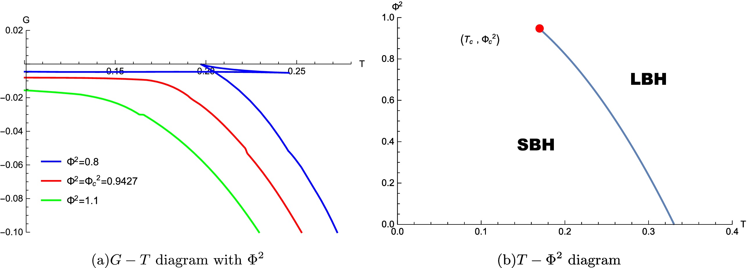
Figure 2. (color online) Critical behaviors for
$ \eta_1=-1 $ ,$ \eta_2=-0.2 $ ,$ \alpha=0.4 $ ,$ \beta =1.6 $ .In the case of two critical radii, Figs. 3(a)−(e) depict the critical behaviors of the Gibbs free energy G. Through a detailed investigation of the processes, we observe a triple critical point
$ ( T_{tr}, {\Phi}_{tr}^2) $ and two types of phase transitions: zero- and first-order. It is important to emphasize that these phase transitions are novel and intriguing as they exhibit a reversal of the reentrant phase transitions [18]. This reversal is illustrated as follows. When$ \Phi^2_{z}<\Phi^2<\Phi^2_{c1} $ , as shown in Fig. 3(a), we observe a "swallowtail" pattern, indicating the occurrence of a VdW phase transition owing to the global minimum value of the Gibbs free energy. The critical point ($ \Phi^2_{z} $ ,$ T_{z} $ ) is depicted in Fig. 3(b). In the range$ \Phi^2_{tr}<\Phi^2<\Phi^2_{z} $ (see Fig. 3(c)), the black hole radius increases along the line from left to right. As the temperature increases from left to right, the value of the free energy, G, decreases along the lower line, considering the minimum of the global Gibbs free energy. The red arrows highlight the physical process of the system with respect to temperature. A swallowtail pattern with a black cross point ($ T=T_c $ ) indicates a first-order phase transition from a small black hole (SBH) to a large black hole (LBH). As the temperature continues to increase, the value of the Gibbs free energy exhibits a discontinuous "jump-up" to the upper line at$ T=T_j $ , signifying a zero-order phase transition from an LBH to an SBH (also referred to as an intermediate black hole (IBH) because it is larger than the former SBH). The process concludes at the point$ T=T_e $ , beyond which there are no black holes for$ T>T_e $ . Thus, the system undergoes a novel "SBH-LBH-SBH" phase transition process, which is the reverse of the "LBH-SBH-LBH" process observed in reentrant phase transitions. Owing to these characteristics, we refer to this process as a "reverse" reentrant phase transition.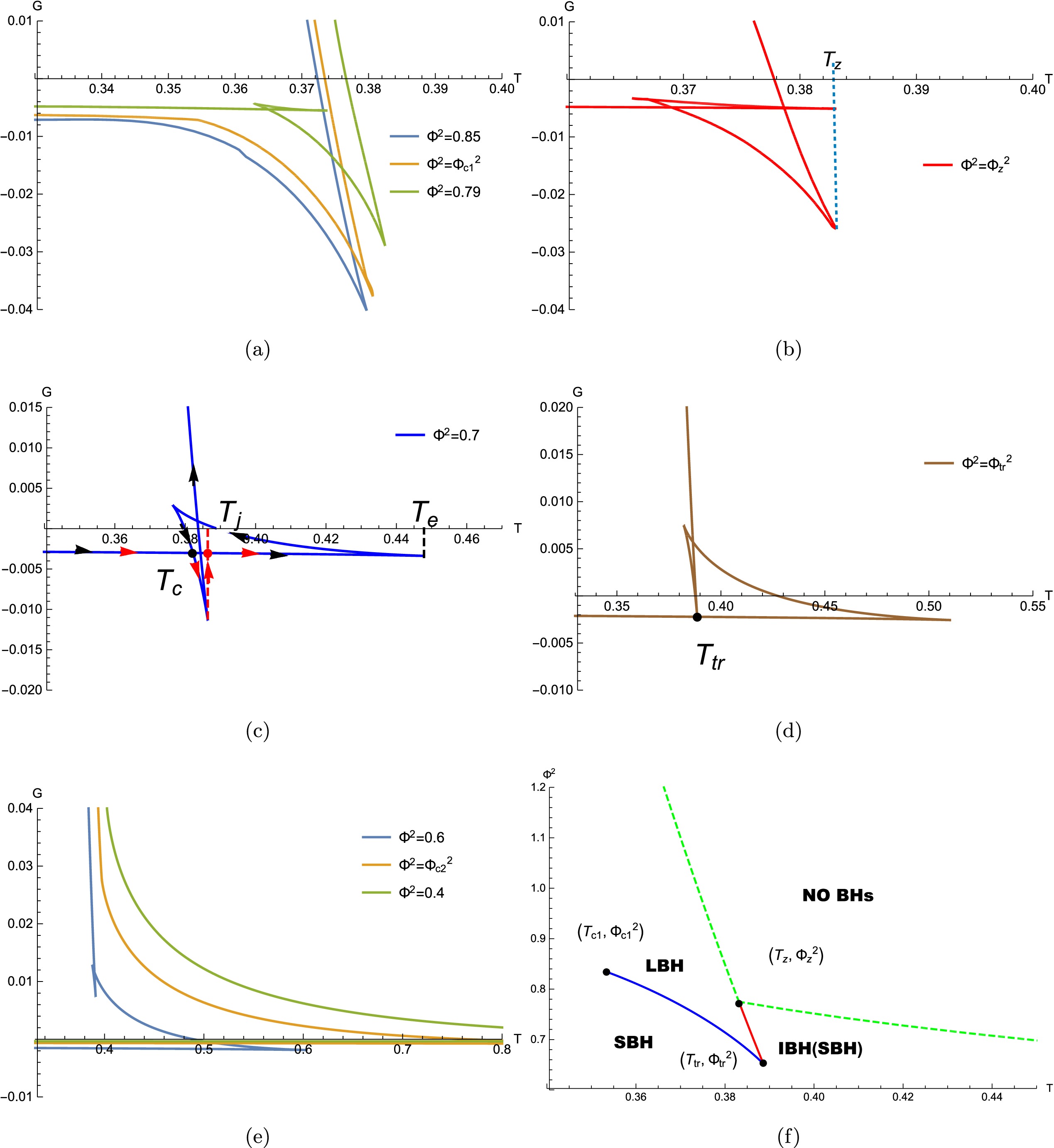
Figure 3. (color online) Diagrams with two critical radii for
$ \eta_1= 1 $ ,$ \eta_2=0.6 $ ,$ \alpha=0.4 $ , and$ \beta=1.6 $ .To provide a clearer explanation, we refer to the phase diagram shown in Fig. 3(f). In this diagram, the blue line represents the coexistence line between SBHs and LBHs, whereas the red line represents the coexistence line between LBHs and IBHs. The starting points of the zero- and first-order phase transitions are denoted as (
$ T_z,\Phi_z^2 $ ) and ($ T_{c1}, \Phi_{c1}^2 $ ), respectively. On the right side of the dashed green line in Fig. 3(f), which represents the right-most points for each line, there are no black holes indicated. For a fixed value of$ \Phi^2 $ , the system undergoes an SBH-LBH-SBH phase transition as the temperature increases, given that$ \Phi_{tr}^2 < \Phi^2 < \Phi_z^2 $ . Additionally, for a fixed temperature of the black hole, the system also experiences an SBH-LBH-SBH phase transition as the critical value of$ \Phi^2 $ increases, within the range$ T_z < T < T_{tr} $ .We also investigate these critical behaviors with the influences of the parameters
$ \eta_1 $ ,$ \eta_2 $ , α, and β, as shown in Tables 1−4. We find that all of the critical temperatures ($ T_{c1} $ ,$ T_{c2} $ ,$ T_{z} $ , and$ T_{tr} $ ) decrease and all of the critical$ \Phi^2 $ values increase with increasing$ \eta_1 $ . However, all of the critical temperatures increase and all of the critical$ \Phi^2 $ values decrease with increasing$ \eta_2 $ , α, and β.$ \eta_1 $ 

$ (\Phi^2_{c1}, T_{c1}) $ 

$ (\Phi^2_{c2}, T_{c2}) $ 

$ (\Phi^2_{z}, T_{z}) $ 

$ (\Phi^2_{tr}, T_{tr}) $ 

0.9 (0.828078, 0.356703) (0.236356, 0.422563) (0.748531, 0.402621) (0.522954, 0.410699) 1 (0.833637, 0.353597) (0.482191, 0.397275) (0.774902, 0.383129) (0.651802, 0.388623) 1.1 (0.839832, 0.350298) (0.642647, 0.377306) (0.799376, 0.36794) (0.736704, 0.371418) Table 1. Critical points with
$ \eta_1 $ for$ \eta_2=0.6 $ ,$ \alpha=0.4 $ , and$ \beta=1.6 $ .$ \eta_2 $ 

$ (\Phi^2_{c1}, T_{c1}) $ 

$ (\Phi^2_{c2}, T_{c2}) $ 

$ (\Phi^2_{z}, T_{z}) $ 

$ (\Phi^2_{tr}, T_{tr}) $ 

0.45 (0.883492, 0.305241) (0.791556, 0.317393) (0.85975, 0.312801) (0.834331, 0.314406) 0.55 (0.848354, 0.337992) (0.597715, 0.369775) (0.800646, 0.359017) (0.718003, 0.363077) 0.65 (0.82029, 0.368788) (0.354553, 0.42554) (0.751269, 0.407869) (0.579794, 0.414905) Table 2. Critical points with
$ \eta_2 $ for$ \eta_1=1 $ ,$ \alpha=0.4 $ , and$ \beta=1.6 $ .$ \alpha $ 

$ (\Phi^2_{c1}, T_{c1}) $ 

$ (\Phi^2_{c2}, T_{c2}) $ 

$ (\Phi^2_{z}, T_{z}) $ 

$ (\Phi^2_{tr}, T_{tr}) $ 

0.395 (0.865026, 0.325119) (0.73737, 0.342417) (0.835141, 0.336136) (0.797332, 0.338403) 0.4 (0.848354, 0.337992) (0.597715, 0.369775) (0.800646, 0.359017) (0.718003, 0.363077) 0.405 (0.832532, 0.351106) (0.407127, 0.401536) (0.765905, 0.385471) (0.613889, 0.391749) Table 3. Critical points with
$ \alpha $ for$ \eta_1=1 $ ,$ \eta_2=0.55 $ , and$ \beta=1.6 $ .$ \beta $ 

$ (\Phi^2_{c1}, T_{c1} $ )

$ (\Phi^2_{c2}, T_{c2} $ )

$ (\Phi^2_{z}, T_{z} $ )

$ (\Phi^2_{tr}, T_{tr} $ )

1.57 (0.867147, 0.328931) (0.752882, 0.344235) (0.839436, 0.33861) (0.806397, 0.340616) 1.61 (0.842724, 0.340924) (0.53447, 0.379301) (0.788289, 0.366616) (0.683107, 0.371478) 1.65 (0.82229, 0.352527) (0.210372, 0.423208) (0.741026, 0.401698) (0.508086, 0.410386) Table 4. Critical points with
$ \beta $ for$ \eta_1=1 $ ,$ \eta_2=0.55 $ , and$ \alpha=0.4 $ . -
In the canonical ensemble with a fixed electric charge Q, the Helmholtz free energy is written as
$ \begin{aligned}[b] F_H =\;& M-TS \\ =\; &\frac{r_h}{4}+\frac{\left(\alpha ^2-1\right) \left(\alpha ^2+1\right) \Lambda r_h^{\frac{3-\alpha ^2}{\alpha ^2+1}}}{4 \left(\alpha ^2-3\right)}\\&+\frac{\left(-\alpha ^4+2 \alpha ^2+3\right) Q^2 r_h^{\frac{\alpha ^2-1}{\alpha ^2+1}}}{2 \left(\alpha ^4-3 \alpha ^2+2\right)}\\ & +\frac{\left(\alpha ^2+1\right) \eta _2 \left(\alpha ^2+2 \alpha \beta -1\right) r_h^{\frac{\alpha ^2+2 \alpha \beta +1}{\alpha ^2+1}}}{4 \left(\alpha ^2+\alpha \beta -1\right) \left(\alpha ^2+2 \alpha \beta +1\right)}\\&+\frac{\alpha \left(\alpha ^2+1\right) \eta _1 (\alpha +2 \beta ) r_h^{\frac{\alpha ^2+2 \alpha \beta +2}{\alpha ^2+1}}}{4 \left(\alpha ^2+2 \alpha \beta +2\right) \left(2 \alpha ^2+2 \alpha \beta -1\right)}. \end{aligned} $

(49) The temperature of the black hole is
$ \begin{aligned}[b] T =\; & \frac{\left(\alpha ^2+1\right) Q^2 r_h^{\frac{\alpha ^2-3}{\alpha ^2+1}}}{2 \pi \left(\alpha ^2-2\right)}-\frac{\left(\alpha ^2+1\right) \Lambda r_h^{\frac{1-\alpha ^2}{\alpha ^2+1}}}{4 \pi }-\frac{\left(\alpha ^2+1\right) r_h^{\frac{\alpha ^2-1}{\alpha ^2+1}}}{4 \pi \left(\alpha ^2-1\right)}\\ &-\frac{\left(\alpha ^2+1\right) \eta _1 r_h^{\frac{\alpha (\alpha +2 \beta )}{\alpha ^2+1}}}{4 \pi \left(2 \alpha ^2+2 \alpha \beta -1\right)}-\frac{\left(\alpha ^2+1\right) \eta _2 r_h^{\frac{2 \alpha (\alpha +\beta )}{\alpha ^2+1}-1}}{4 \pi \left(\alpha ^2+\alpha \beta -1\right)} , \end{aligned} $

(50) and the corresponding heat capacity is
$ C_Q=\frac{8 \pi ^2 T r_h^{\frac{3-\alpha ^2}{\alpha ^2+1}}(\alpha ^2+1)^{-1}}{ -\dfrac{2 \left(\alpha ^2-3\right) Q^2 r_h^{-\frac{2}{\alpha ^2+1}}}{\alpha ^2-2}+\dfrac{\eta _2 \left(\alpha ^2+2 \alpha \beta -1\right) r_h^{\frac{2 \alpha \beta }{\alpha ^2+1}}}{\alpha ^2+\alpha \beta -1}+\dfrac{\alpha \eta _1 (\alpha +2 \beta ) r_h^{\frac{2 \alpha \beta +1}{\alpha ^2+1}}}{2 \alpha ^2+2 \alpha \beta -1}-\left(\alpha ^2-1\right) \Lambda r_h^{\frac{2-2 \alpha ^2}{\alpha ^2+1}}+1}. $

(51) According to Eq. (49), similar to the analysis in the grand canonical system, the term
$ \eta_1 $ vanishes for$ \alpha\rightarrow 0 $ , which also means that the term$ \eta_2 $ is significantly more important in the case without the dilaton field. However, in the case with coupling with the dilaton field, i.e.,$ \alpha\neq 0 $ , considering the asymptotic behaviors of the Helmholtz free energy, the term$ \eta_1 $ plays a more important role than$ \eta_2 $ as$ r_h\rightarrow \infty $ .We can use the conditions of the inflection point in the VdW system,
$ \frac{\partial T}{\partial r_h}\left|_{Q=Q_c,r_h=r_c}\right. =\frac{\partial^2 T}{\partial r_h^2}\left|_{Q={Q_c},r_h=r_c}\right. =0. $

(52) For a given fixed Q, we can obtain the critical
$ Q_{c} $ and the equation of the critical radius of the black hole as$ \begin{aligned}[b] Q_{c}^2=\;&\frac{\left(\alpha ^2-2\right) r_c^{\frac{2}{\alpha ^2+1}}}{2 \left(\alpha ^2-3\right)} -\frac{\left(\alpha ^4-3 \alpha ^2+2\right) \Lambda r_c^{\frac{4-2 \alpha ^2}{\alpha ^2+1}}}{2 \left(\alpha ^2-3\right)} \\&+\frac{\left(\alpha ^2-2\right) \eta _2 \left(\alpha ^2+2 \alpha \beta -1\right) r_c^{\frac{2 \alpha \beta +2}{\alpha ^2+1}}}{2 \left(\alpha ^2-3\right) \left(\alpha ^2+\alpha \beta -1\right)}\\ &+\frac{\alpha \left(\alpha ^2-2\right) \eta _1 (\alpha +2 \beta ) r_c^{\frac{2 \alpha \beta +3}{\alpha ^2+1}}}{2 \left(\alpha ^2-3\right) \left(2 \alpha ^2+2 \alpha \beta -1\right)} , \end{aligned} $

(53) $ \begin{aligned}[b]0=\;& \frac{\eta _2 (\alpha \beta +1) \left(\alpha ^2+2 \alpha \beta -1\right) r_c^{\frac{2 \alpha \beta }{\alpha ^2+1}}}{\alpha ^2+\alpha \beta -1}\\&+\frac{\alpha \eta _1 (\alpha +2 \beta ) (2 \alpha \beta +3) r_c^{\frac{2 \alpha \beta +1}{\alpha ^2+1}}}{4 \alpha ^2+4 \alpha \beta -2}\\&+\left(\alpha ^4-3 \alpha ^2+2\right) \Lambda r_c^{\frac{2-2\alpha^2}{\alpha ^2+1}}+1. \end{aligned}$

(54) When
$ \alpha=0 $ in the AdS space-time, from Eq. (54), we find that it only has one positive root,$ r_c=\frac{\sqrt{{\eta_2}+1}}{2} $ , which depends only on$ \eta_2 $ . Then, the critical values of$ Q^2 $ and the corresponding temperature are respectively calculated as$ Q^2_{c}=\frac{1}{24} ({\eta_2}+1)^2,\quad T_c=\frac{ 2\sqrt{{\eta_2}+1}}{3 \pi }+\frac{ {\eta_1}}{4 \pi }, $

(55) which suggest that there may be first-order SBH/LBH phase transitions in this case, as shown in Fig. 4.
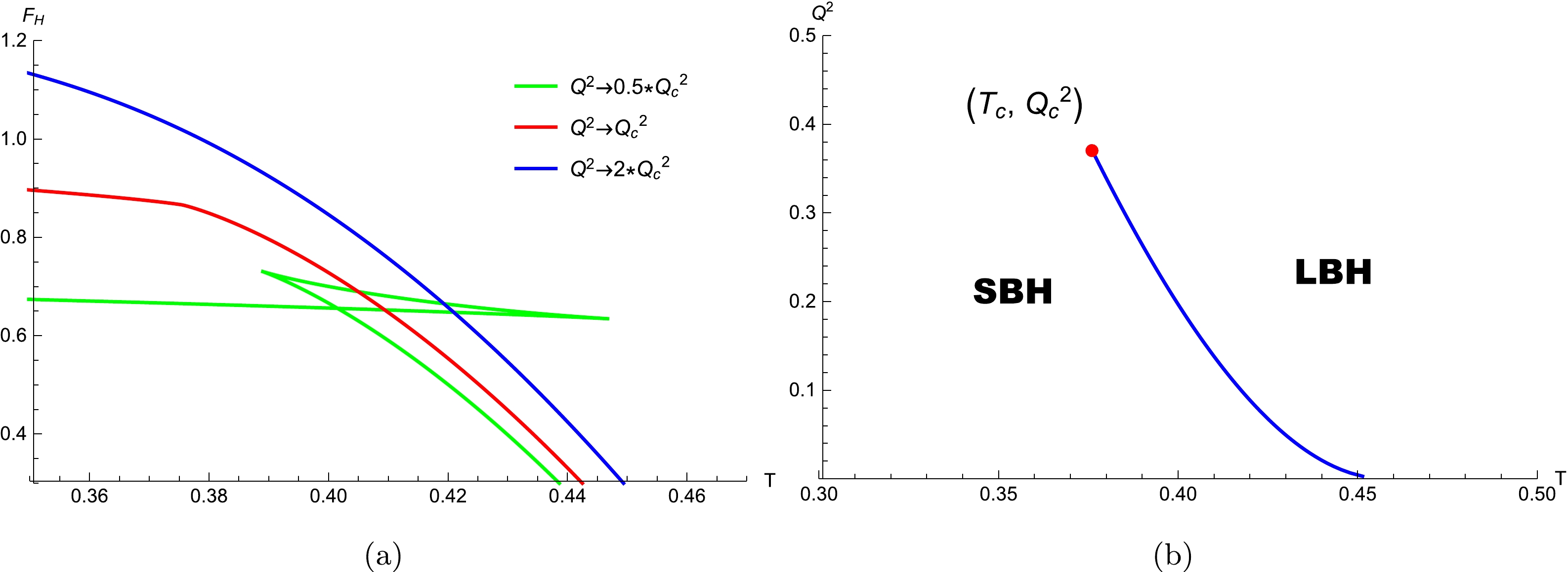
Figure 4. (color online) Critical behaviors with
$ Q^2 $ for$ \alpha=0 $ ,$ \eta_1=0.1 $ , and$ \eta_2=2 $ .When
$ \alpha \neq 0 $ , similar to that in the grand canonical ensemble when studying the critical behaviors, there are several conditions to be considered, i.e., all of the roots of Eq. (54), the$ Q^2_c $ of Eq. (53), and the temperatures of black holes corresponding to the critical points must be positive. Based on these, through numerical analysis, there are at most two critical radii. Taking the case of$ \alpha = 0.6 $ and$ \beta = 0.8 $ as an example, there can be at most two critical radii for$ \eta_1 >0 $ . By investigating the Helmholtz free energy, as shown in Fig. 5 , we find that there are also reverse reentrant phase transitions among SBHs, LBHs, and SBHs. We also investigate the influences of the parameters$ \eta_1 $ ,$ \eta_2 $ , α, and β on these critical behaviors, as shown in Tables 5−8. All of the critical temperatures ($ T_{c1} $ ,$ T_{c2} $ ,$ T_{z} $ , and$ T_{tr} $ ) decrease and all of the critical charges ($ Q^2_{c1} $ ,$ Q^2_{c2} $ ,$ Q^2_{z} $ , and$ Q^2_{tr} $ ) increase with increasing$ \eta_1 $ . However, all of the critical temperatures increase and all of the critical charges ($ Q^2 $ s) decrease with increasing$ \eta_2 $ , α, and β.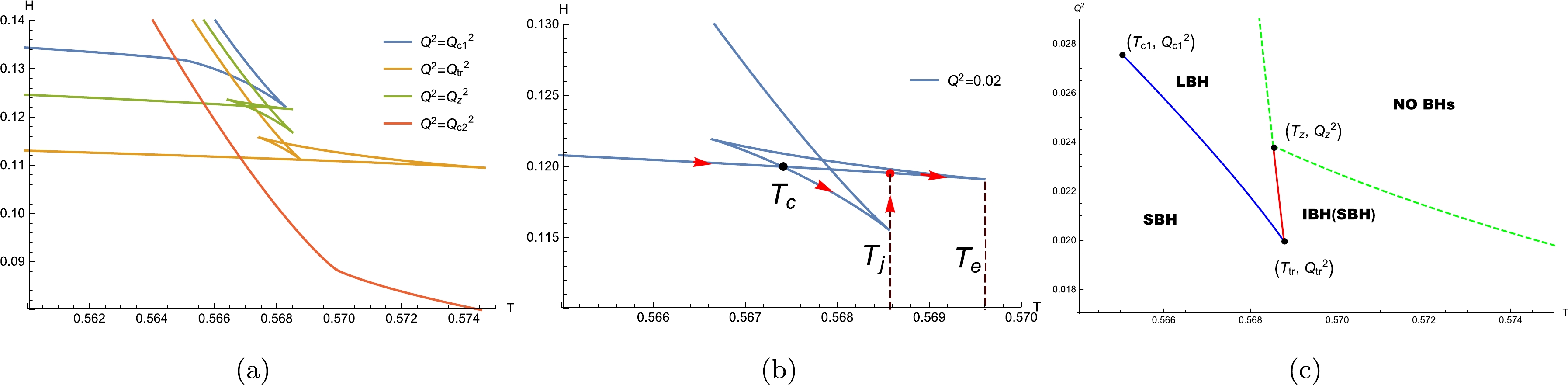
Figure 5. (color online) Critical behaviors for
$ \eta_1= 0.58 $ ,$ \eta_2=0.41 $ ,$ \alpha =0.6 $ , and$ \beta =0.8 $ .$ \eta_1 $ 

$ (Q^2_{c1}, T_{c1}) $ 

$ (Q^2_{c2}, T_{c2}) $ 

$ (Q^2_{z}, T_{z}) $ 

$ (Q^2_{tr}, T_{tr}) $ 

0.58 (0.0275472, 0.565051) (0.00461282, 0.569917) (0.0238421, 0.568524) (0.0199481, 0.568775) 0.59 (0.0282922, 0.563862) (0.013105, 0.567242) (0.0254134, 0.566206) (0.0227447, 0.566408) 0.6 (0.0291293, 0.562626) (0.0200776, 0.564737) (0.0270936, 0.564038) (0.0254712, 0.564185) Table 5. Critical points with
$ \eta_1 $ for$ \eta_2=0.41 $ ,$ \alpha=0.6 $ , and$ \beta=0.8 $ .$ \eta_2 $ 

$ (Q^2_{c1}, T_{c1}) $ 

$ (Q^2_{c2}, T_{c2}) $ 

$ (Q^2_{z}, T_{z}) $ 

$ (Q^2_{tr}, T_{tr}) $ 

0.4 (0.0297303, 0.557388) (0.0201646, 0.559553) (0.0276001, 0.558839) (0.0258868, 0.558989) 0.41 (0.0282922, 0.563862) (0.013105, 0.567242) (0.0254134, 0.566206) (0.0227447, 0.566408) 0.42 (0.0270065, 0.570258) (0.00524945, 0.575021) (0.0234473, 0.57365) (0.0197409, 0.573899) Table 6. Critical points with
$ \eta_2 $ for$ \eta_1=0.59 $ ,$ \alpha=0.6 $ , and$ \beta=0.8 $ .$ \alpha $ 

$ (Q^2_{c1}, T_{c1}) $ 

$ (Q^2_{c2}, T_{c2}) $ 

$ (Q^2_{z}, T_{z}) $ 

$ (Q^2_{tr}, T_{tr}) $ 

0.599 (0.029664, 0.559358) (0.0198809, 0.561567) (0.0275017, 0.560842) (0.0257504, 0.560993) 0.6 (0.0282922, 0.563862) (0.013105, 0.567242) (0.0254134, 0.566206) (0.0227447, 0.566408) 0.601 (0.0270375, 0.568381) (0.00544345, 0.573117) (0.0234916, 0.571751) (0.0198093, 0.571999) Table 7. Critical points with
$ \alpha $ for$ \eta_1=0.59 $ ,$ \eta_2= 0.41 $ , and$ \beta=0.8 $ .$ \beta $ 

$ (Q^2_{c1}, T_{c1}) $ 

$ (Q^2_{c2}, T_{c2}) $ 

$ (Q^2_{z}, T_{z}) $ 

$ (Q^2_{tr}, T_{tr}) $ 

0.797 (0.0297257, 0.5606) (0.0205733, 0.562678) (0.0276622, 0.56199) (0.0260213, 0.562135) 0.801 (0.0278492, 0.564943) (0.0103712, 0.568806) (0.0247118, 0.567649) (0.0216714, 0.567869) 0.804 (0.0266061, 0.568168) (0.00141926, 0.573625) (0.0227377, 0.572095) (0.0185209, 0.572364) Table 8. Critical points with
$ \beta $ for$ \eta_1=0.59 $ ,$ \eta_2= 0.41 $ , and$ \alpha=0.6 $ . -
In this paper, we discuss Maxwell-dilaton massive gravity including a nonminimal coupling term between the graviton and the dilaton field and obtain charged solutions of a dilatonic black hole in four dimensional spacetime. Here, the dilaton potential
$ V(\varphi) $ takes a Liouville-type form, where the last two terms of the potential are associated with the graviton terms.Subsequently, we discuss the singularity of the solution from the Kretschmann scalar and find that the horizons of black holes are simply singularities of coordinates, whereas there is an essential singularity located at the origin. Moreover, the asymptotic behavior of the solutions is neither asymptotically flat nor asymptotically (A)dS. We show that the black hole solutions can provide one horizon, two horizons, and extreme and naked singularity black holes for suitably fixed parameters. To verify the first law of black hole thermodynamics, we calculate the thermodynamic quantities of these dilatonic black holes, such as the entropy, temperature, and mass. Then, we pay further attention to phase space and find richer and more interesting critical phenomena the in grand canonical and canonical ensembles.
In the grand canonical ensemble, there are no VdW-like critical behaviors of black holes without the coupling effect between the graviton and the dilaton field (i.e.,
$ \gamma = 0 $ ). However, there are more critical phenomena when$ \alpha\neq 0 $ . There may be one-order VdW-like phase transitions between SBHs and LBHs. More interestingly, by investigating the Gibbs free energy, there may also be new and interesting critical behaviors with a triple critical point and two types of phase transitions (zero- and one-order), known as a zero-order reverse reentrant phase transition among SBHs, LBHs, and SBHs, because its thermodynamic process is the reverse of that of the reentrant phase transition owing to the minimum of the global Gibbs free energy. In the canonical ensemble, there are only VdW-like phase transitions in the phase space of black holes without the coupling. However, by investigating the Helmholtz free energy, we find that there are also reverse reentrant phase transitions among SBHs, LBHs, and SBHs when$ \alpha\neq 0 $ .
Thermodynamics of charged black holes in Maxwell-dilaton-massive gravity
- Received Date: 2024-02-28
- Available Online: 2024-07-15
Abstract: Considering the nonminimal coupling of the dilaton field to the massive graviton field in Maxwell-dilaton-massive gravity, we obtain a class of analytical solutions of charged black holes, which are neither asymptotically flat nor (A)dS. The calculated thermodynamic quantities, such as mass, temperature, and entropy, verify the validity of the first law of black hole thermodynamics. Moreover, we further investigate the critical behaviors of these black holes in the grand canonical and canonical ensembles and find a novel critical phenomenon never before observed, known as the "reverse" reentrant phase transition with a tricritical point. It implies that the system undergoes a novel "SBH-LBH-SBH" phase transition process and is the reverse of the "LBH-SBH-LBH" process observed in reentrant phase transitions.


 DownLoad: