


 Abstract
 HTML
HTML Reference
 Related
 PDF
PDF


-
Quantum coherence, arising from the superposition principle of quantum states, is an important feature of the quantum world and is the basis of the fundamental phenomena of quantum interference [1]. Similar to quantum entanglement, quantum coherence is an important quantum resource that can be applied in quantum information processing, solid state physics, quantum optics, nanoscale thermodynamics, and biological systems [2–12]. Although quantum coherence is of great importance, it did not attract further attention until Baumgratz et al. proposed a rigorous resource theory framework for the quantization of coherence, such as the
$ l_1 $ norm of coherence and relative entropy of coherence [13]. For complex multipartite systems, the$ l_1 $ norm of coherence is more directly calculated and is easier to obtain analytical expression for than the relative entropy of coherence. However, as the quantum information task becomes increasingly complex, we must deal with it using multipartite coherence.Observer-dependent quantum entanglement can be discussed in the background of an expanding universe [14–17]. The theory of inflationary cosmology and our current observations suggest that our universe may approach de Sitter space with a positive cosmological constant in the far past and far future, which is the unique maximally symmetric curved spacetime. Any two mutually separated R and L regions are eventually causally disconnected in de Sitter space [18], where the universe expands exponentially. This is most appropriately described by spanning open universe coordinates for two open charts in de Sitter space. The positive frequency mode functions of a free massive scalar field correspond to the Bunch-Davies vacuum (the Euclidean vacuum) that supports in both the R and L regions. Using these, entanglement entropy between two causally disconnected regions in de Sitter space has been studied in the Bunch-Davies vacuum and α-vacua [19–24]. Motivated by this, quantum steering, entanglement, and discord were also studied [25–29]. Because it has been shown that quantum entanglement between causally separated regions (beyond the size of the Hubble horizon) exists in de Sitter space, there may be observable effects of quantum correlations on the cosmic microwave background (CMB) in our expanding universe.
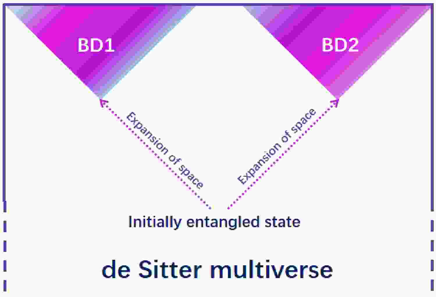
The vacuum fluctuations in our expanding universe may be entangled with those in another part of the multiverse [19]. In other words, we can consider quantum entanglement between two causally disconnected de Sitter spaces (BD1 and BD2) as depicted in Fig. 1 [26, 30]. A quantum system comprises subsystems BD1 and BD2. Assume that the Universe is BD1 and we have no access to BD2. In fact, quantum entanglement of the reduced density matrix influences the shape of the spectrum on large scales, which is comparable to or greater than the curvature radius [20]. This may be the observational signature of the multiverse. In addition, quantum coherence may be determined by the observers in the process of bubble nucleation. It is well known that quantum coherence reflects the nonclassical world better than quantum entanglement, which is considered to be derived from the nonlocal superposition principle of quantum states. In other words, quantum entanglement is a special kind of quantum coherence (genuine coherence) [31–33]. In general, quantum entanglement and coherence show similar properties in a relativistic setting [34–40]. It is not clear whether multipartite coherence and quantum entanglement have similar properties in the multiverse. Therefore, demonstrating the observer's dependence on multipartite coherence in the multiverse is one of the aims of our study.

Figure 1. (color online) Causal diagram of the inflationary multiverse.
Another goal of our study is to better understand the multiverse through multipartite coherence. According to the string landscape and inflationary cosmology, our universe may not be the only one, but part of the multiverse [41–45]. In the structure of the multiverse model, there may be many causally disconnected de Sitter bubbles (de Sitter universes). Until recently, the multiverse was merely untestable philosophical conjecture. However, in the multiverse, quantum coherence between N causally separated universes may generate detectable signatures. Some of their quantum states far from the Bunch-Davies vacuum may be entangled with another universes [19]. Then, we introduce N observers who determine quantum coherence between N causally disconnected de Sitter spaces. We assume n observers inside de Sitter universes and aim to discover how the inner n observers detect the signature of quantum coherence with other
$ N-n $ de Sitter universes.In this paper, we discuss quantum coherence of the N-partite Greenberger-Horne-Zeilinger (GHZ) and W states of massive scalar fields in de Sitter universes. We assume that
$ N-n $ observers are in their respective static universes, whereas n observers are in their expanding universes. Here, an observer corresponds to a universe. We calculate N-partite coherence and obtain its analytical expression in the de Sitter background. We find that with an increase in the curvature, N-partite coherence increases monotonically, whereas quantum correlation decreases monotonically as the curvature increases in de Sitter universes [25–28]. Therefore, we can gain a deeper understanding of the multiverse from the perspective of quantum resources. Although this research may involve quantities that cannot be directly detected in the multiverse, it provides profound insights into the fundamental nature of quantum systems in different spacetime backgrounds.Interestingly, quantum coherence of the N-partite GHZ state in de Sitter universes has nonlocal and local coherence that can exist in subsystems, whereas quantum coherence of the N-partite GHZ state in Rindler spacetime is genuinely global and cannot exist in any subsystems. We quantify nonlocal coherence in terms of the correlated coherence of the multipartite systems in the multiverse. N-partite coherence of the W state in de Sitter universes is not monogamous. However, the correlated coherence of the N-partite W state is equal to the sum of the correlated coherence of all the bipartite subsystems in de Sitter universes. With increasing n, quantum coherence of the W state decreases or increases monotonically depending on curvature, whereas N-partite coherence of the GHZ state increases monotonically for any curvature. These results reveal some unique phenomena of multipartite coherence in de Sitter universes, providing the possibility of discovering the multiverse.
The paper is organized as follows. In Sec. II, we briefly introduce the quantization of the free massive scalar field in de Sitter space. In Sec. III, we study quantum coherence of the tripartite GHZ and W states in the multiverse. In Sec. IV, we extend the relevant research to N-partite systems. Finally, Sec. V presents a brief conclusion.
-
We consider a free scalar field ϕ with mass m in the Bunch-Davies vacuum of de Sitter space represented by the metric
$ g_{\mu\nu} $ . The action of the field is given by$ S=\int {\rm d}^4 x\sqrt{-g}\left[\,-\frac{1}{2}\,g^{\mu\nu} \partial_\mu\phi\,\partial_\nu \phi -\frac{m^2}{2}\phi^2\,\right]\,. $

(1) The coordinate systems of the open chart in de Sitter space can be obtained via analytic continuation from the Euclidean metric and divided into two parts that we refer to as
$ R,L $ . The R and L regions, which are covered by the coordinates$ (t_{L}, r_{L}) $ and$ (t_{R}, r_{R}) $ , respectively, in de Sitter space, are causally disconnected, and their metrics are given, respectively, by$ \begin{aligned}[b] {\rm d}s^2_R &= H^{-2}\left[-{\rm d}t^2_R+\sinh^2t_R\left({\rm d}r^2_R+\sinh^2r_R\,{\rm d}\Omega^2\right) \right]\,,\\ {\rm d}s^2_L&= H^{-2}\left[-{\rm d}t^2_L+\sinh^2t_L\left({\rm d}r^2_L+\sinh^2r_L\,{\rm d}\Omega^2\right) \right]\,, \end{aligned} $

(2) where
$ H^{-1} $ is the Hubble radius, and${\rm d}\Omega^2$ is the metric on the two-sphere [18]. To obtain the analytic continuation solutions in the R or L region, we must resolve this process in the Euclidean hemisphere. It is natural to choose the Euclidean vacuum (Bunch-Davies vacuum) with de Sitter invariance as the initial condition. Therefore, we must find the positive frequency mode functions corresponding to the Euclidean vacuum. By separating the variables, we obtain$ \phi=\frac{H}{\sinh t}\,\chi_{p}(t)Y_{p\ell m}(r,\Omega), $

(3) and the solutions of the Klein-Gordon equations for
$ \chi_{p}(t) $ and$ Y_{p\ell m}(r,\Omega) $ in the R or L region are found to be$\bigg[\frac{\partial^{2}}{\partial t^{2}}+3\coth t \frac{\partial}{\partial t}+\frac{1+p^{2}}{\sinh^{2}t}+\frac{m^{2}}{H^{2}}\bigg]\chi_{p}(t)=0, $

(4) $ \begin{aligned}[b] & \bigg[\frac{\partial^{2}}{\partial r^{2}}+2\coth t \frac{\partial}{\partial r}-\frac{1}{\sinh^{2}t}{\bf{L^{2}}}\bigg]Y_{p\ell m}(r,\Omega)\\ & \quad=-(1+p^{2})Y_{p\ell m}(r,\Omega), \end{aligned} $

(5) where
$ Y_{p\ell m}(r,\Omega) $ are eigenfunctions on the three-dimensional hyperboloid, and$ {\bf{L^{2}}} $ is the Laplacian operator on the unit two-sphere [19, 46].The positive frequency mode functions corresponding to the Euclidean vacuum supported both on the R and L regions are given by
$\chi_{p,\sigma}(t)=\left\{ \begin{aligned} & \frac{{\rm e}^{\pi p}-{\rm i}\sigma {\rm e}^{-{\rm i}\pi\nu}}{\Gamma \left(\nu+{\rm i}p+\dfrac{1}{2}\right)}P_{\nu-\frac{1}{2}}^{{\rm i}p}(\cosh t_R) -\frac{{\rm e}^{-\pi p}-{\rm i}\sigma {\rm e}^{-{\rm i}\pi\nu}}{\Gamma \left(\nu-{\rm i}p+\dfrac{1}{2}\right)}P_{\nu-\frac{1}{2}}^{-{\rm i}p}(\cosh t_R) \,,\\ & \frac{\sigma {\rm e}^{\pi p}-{\rm i}\,{\rm e}^{-{\rm i}\pi\nu}}{\Gamma \left(\nu+{\rm i}p+\dfrac{1}{2}\right)}P_{\nu-\frac{1}{2}}^{{\rm i}p}(\cosh t_L) -\frac{\sigma {\rm e}^{-\pi p}-{\rm i}\,{\rm e}^{-{\rm i}\pi\nu}}{\Gamma \left(\nu-{\rm i}p+\dfrac{1}{2}\right)}P_{\nu-\frac{1}{2}}^{-{\rm i}p}(\cosh t_L) \,, \end{aligned} \right.$

(6) where
$P^{\pm {\rm i}p}_{\nu-\frac{1}{2}}$ are the associated Legendre functions, and$ \sigma=\pm 1 $ is used for distinguishing the independent solutions in each open region. Their Klein-Gordon norms are evaluated to give$ [\chi_{p,\sigma}(t),\chi_{p,\sigma'}(t)]=N_{p}\delta_{\sigma\sigma'} $ with the normalization factor$ N_{p}=\dfrac{4\sinh\pi p\,\sqrt{\cosh\pi p-\sigma\sin\pi\nu}}{\sqrt{\pi}\,|\Gamma(\nu+{\rm i} p+\frac{1}{2})|}\, $ [18]. In the above solutions, ν is a mass parameter that is given by$ \nu=\sqrt{\frac{9}{4}-\frac{m^2}{H^2}}\,. $

(7) Note that the two special values of the mass parameters
$ \nu= 1/2 $ and$ \nu= 3/2 $ correspond to the conformally coupled massless scalar and minimally coupled massless limit, respectively. Here, p is the momentum of the scalar field. The curvature effect in three-dimensional hyperbolic space starts to appear around$ p\sim1 $ . When the momentum p decreases, the curvature effect becomes stronger. Therefore, we can probe the curvature effect on multipartite coherence by varying the momentum p [25–29].The scalar field can be expanded in terms of the annihilation and creation operators
$ \begin{aligned}[b] \hat\phi(t,r,\Omega) =\,& \frac{H}{\sinh t}\int {\rm d}p \sum\limits_{\sigma,\ell,m}\left[\,a_{\sigma p\ell m}\,\chi_{p,\sigma}(t) +a_{\sigma p\ell -m}^\dagger\,\chi^*_{p,\sigma}(t)\right] \\ & \times Y_{p\ell m}(r,\Omega) \,, \end{aligned} $

(8) where
$ a_{\sigma p\ell m} $ satisfies$ a_{\sigma p\ell m}|0\rangle_{{\rm{BD}}}=0 $ in the Bunch-Davies vacuum. We introduce a Fourier mode field operator as follow$ \phi_{ p\ell m} (t)\equiv\sum\limits_{\sigma}\left[\,a_{\sigma p\ell m}\,\chi_{p,\sigma}(t) +a_{\sigma p\ell -m}^\dagger\,\chi^*_{p,\sigma}(t)\right] \,. $

(9) For simplicity, hereafter, we omit the indices p,
$ \ell $ , and m in the operators$ \phi_{p\ell m} $ ,$ a_{\sigma p\ell m} $ , and$ a_{\sigma p\ell -m}^\dagger $ . For example, the mode functions and the associated Legendre functions can be rewritten as$ P_{\nu-1/2}^{ip}(\cosh t_{R,L})\rightarrow P^{R, L} $ ,$P_{\nu-1/2}^{-ip}(\cosh t_{R,L}) \rightarrow P^{R*, L*}$ , and$ \chi_{p,\sigma}(t)\rightarrow \chi^{\sigma} $ .The two lines of Eq. (6) can be expressed in the one line
$ \chi^{\sigma} = \tilde{N}_p^{-1} \sum\limits_{q=R,L} \left[\, \alpha_q^\sigma\,P^q + \beta_q^\sigma\,P^{*\,q} \,\right]\,, $

(10) where
$\tilde{N}_p^{-1}=\dfrac{|\Gamma(1+{\rm i}p)|}{\sqrt{2p}}$ and$ \alpha_R^\sigma = \frac{{\rm e}^{\pi p} -{\rm i}\sigma {\rm e}^{-{\rm i}\pi \nu}}{\Gamma \left(\nu+{\rm i}p +\dfrac{1}{2}\right)},\quad \beta_R^\sigma =-\frac{{\rm e}^{-\pi p} -{\rm i}\sigma {\rm e}^{-{\rm i}\pi \nu}}{\Gamma \left(\nu-{\rm i}p +\dfrac{1}{2}\right)} \,\,,$

(11) $ \alpha_L^\sigma =\sigma\,\frac{{\rm e}^{\pi p} -{\rm i}\sigma {\rm e}^{-{\rm i}\pi \nu}}{\Gamma \left(\nu+{\rm i}p +\dfrac{1}{2}\right)} \,,\quad \beta_L^\sigma =-\sigma\,\frac{{\rm e}^{-\pi p} -{\rm i}\sigma {\rm e}^{-{\rm i}\pi \nu}}{\Gamma \left(\nu-{\rm i}p +\dfrac{1}{2}\right)} \,\,. $

(12) The complex conjugate of Eq. (10) reads as
$ \chi^{*\,\sigma}=N_p^{-1}\sum\limits_{q=R,L} \left[\, {\beta^{*}_q}^{\sigma}\,P^q + {\alpha^{*}_q}^{\sigma}\,P^{*\,q} \,\right]\,. $

(13) Then, Eq. (6) and its conjugate can be placed into the simple matrix form [22, 26]
$ \chi^I=N_p^{-1}\,M^I{}_J\,P^J\,, $

(14) where the capital indices
$ (I,J) $ run from 1 to 4, and$ \begin{split} & \chi^I=\left(\,\chi^\sigma\,,\chi^{*\,\sigma}\,\right)\,,\quad M^I{}_J=\left( \begin{array}{*{20}{l}} {\alpha^\sigma_q} &{ \beta^\sigma_q} \\ {{\beta^{*}_q}^{\sigma}} & {{\alpha^{*}_q}^{\sigma}} \end{array}\right)\,,\\ & P^J=\left(\,P^R\,,P^L\,,P^{*\,R}\,, P^{*\,L}\,\right)\,. \end{split} $

(15) Now, we introduce the new annihilation and creation operators (
$ b_q,b_q^\dagger $ ) that satisfy$ b_q|0\rangle_{q}=0 $ in different regions. Because the Fourier mode field operator is the same under the change of mode functions, we can relate the annihilation and creation operators ($ b_q,b_q^\dagger $ ) and$ (a_\sigma,a_\sigma^\dagger) $ in different references [22, 26]. Therefore, we have$ \begin{split} & \phi(t)=a_I\,\chi^I=N_p^{-1}a_I\,M^I{}_J\,P^J\,=N_p^{-1}b_J\,P^J\,,\\ & a_I=\left(\,a_\sigma\,,\,a_\sigma^\dagger\,\right)\,,\quad b_J=\left(\,b_R\,,\,b_L\,,\,b_R^\dagger\,,\, b_L^\dagger\,\right)\,. \end{split} $

(16) From Eq. (16), we obtain the relation
$ \begin{split} & a_J=b_I\left(M^{-1}\right)^I{}_J\,,\qquad \left(M^{-1}\right)^I{}_J=\left( \begin{array}{*{20}{l}} {\xi_{q\sigma}} & {\delta_{q\sigma} }\\ {\delta_{q\sigma}^* }& {\xi_{q\sigma}^* } \end{array}\right)\,,\\ & \left\{ \begin{array}{l} \xi= \left(\alpha-\beta\,\alpha^{*\,-1}\beta^*\right)^{-1}\,,\\ \delta=-\alpha^{-1}\beta\,\xi^*\,. \end{array} \right. \end{split} $

(17) Using the Bogoliubov transformation between the operators, the Bunch-Davies vacuum and single particle excitation states can be constructed from the states in the R and L regions [28], which can be expressed as
$ |0\rangle_{{\rm{BD}}} = \sqrt{1-|\gamma_{p}|^{2}}\sum\limits_{n=0}^{\infty}\gamma_{p}^{n}|n\rangle_{L}|n\rangle_{R}\,, $

(18) $ \begin{split} \qquad |1\rangle_{{\rm{BD}}}=\,&\frac{1-|\gamma_{p}|^{2}}{\sqrt{2}}\sum\limits_{n=0}^{\infty}\gamma^{n}_{p}\sqrt{n+1}\big[|(n+1)\rangle_{{\rm{L}}}|n\rangle_{{\rm{R}}}\\ & +|n\rangle_{{\rm{L}}}|(n+1)\rangle_{{\rm{R}}}\big], \end{split} $

(19) where
$ |n\rangle_{R} $ and$ |n\rangle_{L} $ correspond to the two modes of the R and L de Sitter open charts, respectively, and the parameter$ \gamma_p $ reads as$ \gamma_p = {\rm i} \frac{\sqrt{2}}{\sqrt{\cosh 2\pi p + \cos 2\pi \nu} + \sqrt{\cosh 2\pi p + \cos 2\pi \nu +2 }}\,. $

(20) Now, we elaborate on the assertion that p can be regarded as the curvature parameter of the de Sitter space. Employing Eq. (18), the reduced density matrix from the Bunch-Davies basis to the basis of the open chart in the L region can be expressed as
$ \rho_{{\rm{L}}}={\rm{Tr_R(|0\rangle_{BD}\langle0|)}}=(1-|\gamma_{p}|^{2})\sum\limits_{n=0}^{\infty}|\gamma_{p}|^{2n}| n\rangle_{{\rm{L}}}\langle n|. $

(21) Similarly, we can also obtain the reduced density matrix from the Minkowski basis to the Rindler basis, which is found to be
$ \rho_{{\rm{I}}}=(1-{\rm e}^{-2\pi \frac{\omega}{a}})\sum\limits_{n=0}^{\infty}{\rm e}^{-2\pi n\frac{\omega}{a}}| n\rangle_{{\rm{I}}}\langle n|, $

(22) where a is the acceleration [36, 38]. From Eqs. (21) and (22), we can obtain
$ a=-\pi\omega/\ln|\gamma_{p}| $ . For the given values of ν and ω, it is evident that the temperature$T_U=\dfrac{a}{2\pi}$ is a monotonically decreasing function of p. That is, a decrease in p will lead to an increase in the curvature effect of de Sitter space. This assertion has been utilized previously [25–29]. -
Utilizing this Bogoliubov transformation given by Eqs. (18) and (19), we discover that the initial state of the Bunch-Davies mode observed by an observer in the global chart corresponds to a two-mode squeezed state in the open charts. These two modes correspond to the fields observed in the R and L charts. If we exclusively examine one of the open charts, for example, L, we cannot access the modes in the causally disconnected R region and must consequently trace over the inaccessible region. This situation is analogous to the relationship between an observer in a Minkowski chart and another in one of the two Rindler charts. In this sense, the global and Minkowski charts encompass the entire spacetime geometry, whereas the open and Rindler charts cover only a portion of the spacetime. From the above analysis, we find that time evolution does not play a direct role in the calculations presented in the paper. The focus is primarily on the initial quantum states and the subsequent tracing out of parts of the density matrix.
In the structure of the multiverse model, there may be many causally disconnected de Sitter bubbles (de Sitter universes), and the inside of a nucleated bubble resembles an open universe. Along this line, we initially consider two typical tripartite GHZ and W states shared by Alice, Bob, and Charlie, who determine quantum coherence between three causally disconnected de Sitter spaces. The technology for preparing GHZ and W states in experiments has become highly established [47, 48]. Quantum coherence can be observed experimentally in flat spacetime [49, 50]. As is well known, the search for multiverse observations remains an open question, and most research on the multiverse is theoretical [26, 30]. Therefore, we believe that understanding the behavior of quantum coherence of GHZ and W states can provide guidance for simulating the multiverse using quantum systems [51–53]. By removing a single particle from the W state, the ensuing bipartite state remains entangled. Thus, the W state demonstrates a remarkable persistence of quantum entanglement in the face of particle loss. Unlike for the W state, quantum entanglement and coherence of the GHZ state only exist in three particles. Then, we set Bob and Charlie to remain in the L regions of two expanded de Sitter universes, and Alice is in the global chart of the other de Sitter space without expansion. In experiments, it is temporarily difficult to realistically place an entangled particle in every universe, but this is just for our theoretical model. If we probe only an open chart, such as L, the observer cannot access the mode in the causally disconnected R region, and the inaccessible R region must be traced over. In other words, in composite quantum systems, we only focus on the modes under consideration; hence, we must trace the remaining modes. A pure state of the observers will then be a mixed state. Therefore, thermal noise introduced by the expanding universe destroys quantum correlations [25–28]. In the following, we explore the properties of tripartite coherence in the multiverse.
-
We assume that three observers, Alice, Bob, and Charlie, share a tripartite GHZ state of the free massive scalar field, defined as
$ \begin{aligned}[b] |GHZ\rangle_{ABC}=\,& \frac{1}{\sqrt{2}}[|0\rangle_{A, {\rm{BD}}_{1}}|0\rangle_{B, {\rm{BD}}_{2}}|0\rangle_{C, {\rm{BD}}_{3}}\\ & +|1\rangle_{A, {\rm{BD}}_{1}}|1\rangle_{B, {\rm{BD}}_{2}}|1\rangle_{C, {\rm{BD}}_{3}}]. \end{aligned} $

(23) Here, Alice, Bob, and Charlie are in the three causally disconnected de Sitter spaces
$ ({\rm{BD}}_{1}) $ ,$ ({\rm{BD}}_{2}) $ , and$ ({\rm{BD}}_{3}) $ , respectively. Then, we consider that Bob and Charlie are in the L regions of expanded de Sitter universes and Alice is in a global chart of the other de Sitter space. For convenience, we omit the subscript BD. Using Eqs. (18) and (19), we can rewrite Eq. (23) as$ \begin{aligned}[b] |GHZ\rangle_{A B \bar{B} C \bar{C}}=&\frac{1-|\gamma_{p}|^{2}}{\sqrt{2}}\sum\limits_{n,m=0}^{\infty}\gamma^{n}_{p}\gamma^{m}_{p}\bigg[|0\rangle_A |n\rangle_{B}| n\rangle_{\bar{B}}|m\rangle_{C}|m\rangle_{\bar{C}}\\ & +\frac{1-|\gamma_{p}|^{2}}{2}\sqrt{n+1}\sqrt{m+1}|1\rangle_A(|n+1\rangle_{B}|n\rangle_{\bar{B}}\\ & +|n\rangle_{B}|n+1\rangle_{\bar{B}})\\ & \otimes (|m+1\rangle_{C}|m\rangle_{\bar{C}}+|m\rangle_{C}|m+1\rangle_{\bar{C}})\bigg], \end{aligned} $

(24) where the modes
$ \bar{B} $ and$ \bar{C} $ are in the R regions. Because the R and L regions are causally disconnected, we must trace over the modes$ \bar{B} $ and$ \bar{C} $ in the R regions and obtain the reduced density matrix as$ \rho_{ABC}=\frac{(1-|\gamma_{p}|^{2})^{2}}{2}\sum\limits_{n,m=0}^{\infty}\gamma_{p}^{2n}\gamma_{p}^{2m}\rho_{n,m}, $

(25) where
$ \begin{split} \rho_{n,m}=&|0\rangle_{A}\langle0||n\rangle_{B}\langle n||m\rangle_{C}\langle m|+\frac{1-|\gamma_{p}|^{2}}{2}\sqrt{n+1}\sqrt{m+1}|0\rangle_{A}\langle1|\\ \otimes&(|n\rangle_{B}\langle n+1|+\gamma_{p}|n+1\rangle_{B}\langle n|)(|m\rangle_{C}\langle m+1|+\gamma_{p}|m+1\rangle_{C}\langle m|)\\ &+\frac{1 - |\gamma_{p}|^{2}}{2}\sqrt{n+1}\sqrt{m+1}|1\rangle_{A}\langle0|(|n+1\rangle_{B}\langle n|\\ &+\gamma_{p}^{*}|n\rangle_{B}\langle n+1|)\otimes(|m+1\rangle_{C}\langle m|+\gamma_{p}^{*}|m\rangle_{C}\langle m+1|)\\ &+\frac{(1-|\gamma_{p}|^{2})^{2}}{4}|1\rangle_{A}\langle1|\otimes[(n+1)(|n+1\rangle_{B}\langle n+1|+|n\rangle_{B}\langle n|)\\ &+\sqrt{n+2}\sqrt{n+1}\times(\gamma_{p}|n+2\rangle_{B}\langle n|+\gamma_{p}^{*}|n\rangle_{B}\langle n+2|)] [(m+1)\\ &(|m+1\rangle_{C}\langle m+1|+|m\rangle_{C}\langle m|)+\sqrt{m+2}\sqrt{m+1}\\ &(\gamma_{p}|m+2\rangle_{C}\langle m|+\gamma_{p}^{*}|m\rangle_{C}\langle m+2|)].\\[-1pt] \end{split} $

(26) Next, we explore the properties of quantum coherence of the GHZ state in the multiverse. Here, we use the
$ l_{1} $ norm of coherence introduced by Baumgratz et al. to quantify quantum coherence [13], which is defined as the sum of the absolute value of all the off-diagonal elements of a system density matrix,$ C(\rho)=\sum\limits_{i\neq j}|\rho_{i,j}|. $

(27) It is essential to emphasize that quantum coherence is contingent upon the selection of a reference basis. Representing the same quantum state with different reference bases can result in different values of quantum coherence. Practically, the selection of the reference basis may be governed by the physics inherent in the problem under consideration. For instance, one might concentrate on the energy eigenbasis when exploring coherence in the context of transport phenomena and thermodynamics. In the quantum depiction of Young's two-slit interference, the path basis is advantageous. In this study, we employ the particle number representation to investigate the dynamics of multipartite coherence for scalar fields in the multiverse. In quantum optics, the coherent superposition of number states with different numbers of photons is crucial, playing significant roles in various optical interference settings [54]. As is widely recognized, coherent and squeezed states of optical fields stand out as typical examples of such coherent superposition. In the case of two-mode optical fields, coherent superposition in photon-number bases can lead to the emergence of entanglement between the photons of the two modes, such as in the case of two-mode squeezed states. This represents an essential resource in various applications. The coherence resulting from the superposition of photon-number states typically leads to a nonuniform distribution of optical intensity concerning position or time. This phenomenon gives rise to interference fringes, which can be detected through appropriate settings. The maturity of technologies in quantum optics provides the foundation for investigating scalar field counterparts in the multiverse.
Employing Eqs. (25) and (27), quantum coherence of the GHZ state becomes
$ \begin{aligned}[b] C(\rho_{ABC})=\;&\frac{1}{2}\{(1-|\gamma_{p}|^{2})^{3}[\sum\limits_{n=0}^{\infty}\gamma_{p}^{2n}\sqrt{n+1}(1+|\gamma_{p}|)]^{2}\\&+ [(1-|\gamma_{p}|^{2})^{2}\sum\limits_{n=0}^{\infty}\gamma_{p}^{2n+1}\sqrt{n+2}\sqrt{n+1}]^{2}\\ &+2(1-|\gamma_{p}|^{2})^{2}\sum\limits_{n=0}^{\infty}\gamma_{p}^{2n+1}\sqrt{n+2}\sqrt{n+1} \}. \end{aligned} $

(28) In the above calculations, we use the relations
$ (1-|\gamma_{p}|^{2})\sum\limits_{n=0}^{\infty}|\gamma_{p}|^{2n}=1, $

(29) and
$ (1-|\gamma_{p}|^{2})^{2}\sum\limits_{n=0}^{\infty}|\gamma_{p}|^{2n}(n+1)=1. $

(30) As shown in Eq. (28), quantum coherence depends on the curvature parameter p and mass parameter ν, which indicates that the curvature effect influences quantum coherence in de Sitter spaces.
In Fig. 2, we plot quantum coherence
$ C(\rho_{ABC}) $ as functions of the mass parameter ν and curvature parameter p. Quantum coherence of the GHZ state decreases monotonically with an increase in the curvature parameter p. In other words, quantum coherence of the GHZ state increases with curvature. This suggests that the curvature effect can improve quantum coherence in the multiverse. Conversely, quantum entanglement and discord decrease with an increase in the curvature in de Sitter spaces [25–28]. In addition, quantum coherence of the GHZ state is more sensitive to the curvature effect for$ \nu\rightarrow1/2 $ (conformally coupled massless limit) and$ \nu\rightarrow3/2 $ (minimally coupled massless limit).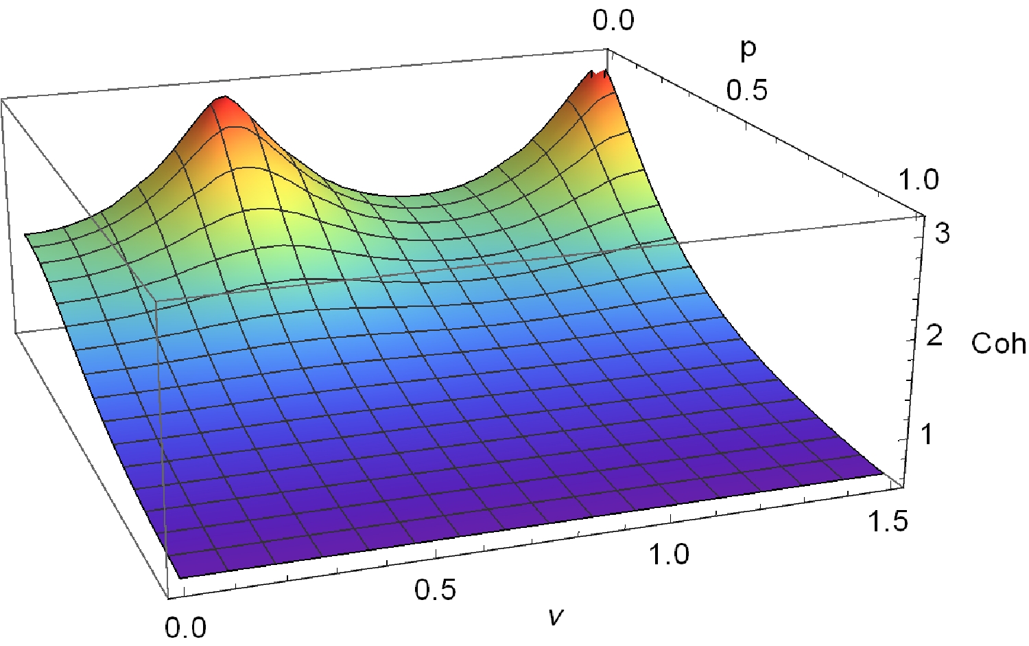
Figure 2. (color online) Quantum coherence
$ C(\rho_{ABC}) $ of the GHZ state as a function of the mass parameter ν and curvature parameter p.Tracing over the modes A, B, or C from
$ \rho_{ABC} $ , we respectively obtain$ \begin{split} \rho_{BC}=&\frac{1}{2}\big\{ (1-|\gamma_{p}|^{2})^{2}\sum\limits_{n=0}^{\infty}\gamma_{p}^{2n}|n\rangle_{B}\langle n|\otimes(1-|\gamma_{p}|^{2})^{2}\\ &\sum\limits_{m=0}^{\infty}\gamma_{p}^{2m}|m\rangle_{C}\langle m|+\sum\limits_{n=0}^{\infty}[\frac{(1-|\gamma_{p}|^{2})^{2}}{2}\gamma_{p}^{2n}(n+1)\\ & (|n\rangle_{B}\langle n|+|n+1\rangle_{B}\langle n+1|)+\frac{(1-|\gamma_{p}|^{2})^{2}}{2}\gamma_{p}^{2n}\sqrt{n+1}\\ &\sqrt{n+2}(\gamma_{p}|n+2\rangle_{B}\langle n|+\gamma_{p}^{*}|n\rangle_{B}\langle n+2|)]\\ &\otimes\sum\limits_{m=0}^{\infty}[\frac{(1-|\gamma_{p}|^{2})^{2}}{2}\gamma_{p}^{2m}(m+1)(|m\rangle_{C}\langle m|+|m+1\rangle_{C}\\ &\langle m+1|)+\frac{(1-|\gamma_{p}|^{2})^{2}}{2}\gamma_{p}^{2m}\sqrt{m+1}\sqrt{m+2}(\gamma_{p}|m\\ &+2\rangle_{C}\langle m|+\gamma_{p}^{*}|m\rangle_{C}\langle m+2|)]\}, \\[-1pt] \end{split} $

(31) $ \begin{aligned}[b] \rho_{AC}=\;& \frac{1}{2}\{|0\rangle_{A}\langle0|\otimes(1-|\gamma_{p}|^{2})^{2}\sum\limits_{m=0}^{\infty}\gamma_{p}^{2m}|m\rangle_{C}\langle m| + |1\rangle_{A}\langle1| \otimes \sum\limits_{m=0}^{\infty}[\left(\frac{(1-|\gamma_{p}|^{2})^{2}}{2}\gamma_{p}^{2m}(m+1)|m\rangle_{C}\langle m|+|m+1\rangle_{C}\langle m+1|\right)\\&+ \frac{(1-|\gamma_{p}|^{2})^{2}}{2}\gamma_{p}^{2m}\sqrt{m+1}\sqrt{m+2}(\gamma_{p}|m+2\rangle_{C}\langle m|+\gamma_{p}^{*}|m\rangle_{C}\langle m+2|)]\}, \end{aligned} $

(32) $ \begin{aligned}[b] \rho_{AB}=\;& \frac{1}{2}\{|0\rangle_{A}\langle0|\otimes(1-|\gamma_{p}|^{2})^{2}\sum\limits_{m=0}^{\infty}\gamma_{p}^{2m}|m\rangle_{B}\langle m| + |1\rangle_{A}\langle1| \otimes \sum\limits_{m=0}^{\infty}[\left(\frac{(1-|\gamma_{p}|^{2})^{2}}{2}\gamma_{p}^{2m}(m+1)|m\rangle_{B}\langle m|+|m+1\rangle_{B}\langle m+1|\right)\\&+ \frac{(1-|\gamma_{p}|^{2})^{2}}{2}\gamma_{p}^{2m}\sqrt{m+1}\sqrt{m+2}(\gamma_{p}|m+2\rangle_{B}\langle m|+\gamma_{p}^{*}|m\rangle_{B}\langle m+2|)]\}. \end{aligned} $

(33) Similarly, we obtain the density matrices of the subsystem A, B, and C
$ \rho_{A}=\frac{1}{2}(|0\rangle_{A}\langle0|+|1\rangle_{A}\langle1|), $

(34) $ \begin{aligned}[b] \rho_{B}=\;&\frac{1}{2}\{|0\rangle_{B}\langle0|+\sum\limits_{m=0}^{\infty}[\left(\frac{(1-|\gamma_{p}|^{2})^{2}}{2}\gamma_{p}^{2m}(m+1)|m\rangle_{B}\langle m|+|m+1\rangle_{B}\langle m+1|\right)\\&+ \frac{(1-|\gamma_{p}|^{2})^{2}}{2}\gamma_{p}^{2m}\sqrt{m+1}\sqrt{m+2}(\gamma_{p}|m+2\rangle_{B}\langle m|+\gamma_{p}^{*}|m\rangle_{B}\langle m+2|)]\}, \end{aligned} $

(35) $ \begin{aligned}[b] \rho_{C}=\;&\frac{1}{2}\{|0\rangle_{C}\langle0|+\sum\limits_{m=0}^{\infty}[\left(\frac{(1-|\gamma_{p}|^{2})^{2}}{2}\gamma_{p}^{2m}(m+1)|m\rangle_{C}\langle m|+|m+1\rangle_{C}\langle m+1|\right)\\&+ \frac{(1-|\gamma_{p}|^{2})^{2}}{2}\gamma_{p}^{2m}\sqrt{m+1}\sqrt{m+2}(\gamma_{p}|m+2\rangle_{C}\langle m|+\gamma_{p}^{*}|m\rangle_{C}\langle m+2|)]\}. \end{aligned} $

(36) Using Eq. (27), we obtain bipartite coherence as
$ C(\rho_{AB})=C(\rho_{AC})=\frac{(1-|\gamma_{p}|^{2})^{2}}{2}\sum\limits_{n=0}^{\infty}\sqrt{n+2}\sqrt{n+1}|\gamma_{p}|^{2n+1}, $

(37) $ \begin{split} C(\rho_{BC})=\;&\frac{1}{2}\big \{[(1-|\gamma_{p}|^{2})^{2}\sum\limits_{n=0}^{\infty}\sqrt{n+2}\sqrt{n+1} |\gamma_{p}|^{2n+1}]^{2}\\&+2(1-|\gamma_{p}|^{2})^{2}\sum\limits_{n=0}^{\infty}\sqrt{n+2}\sqrt{n+1} |\gamma_{p}|^{2n+1}\big\}.\\[-1pt] \end{split} $

(38) From Eqs. (34)−(36), we find
$ C(\rho_{A}) $ = 0 and$ C(\rho_{AB}) = C(\rho_{AC})=C(\rho_{B})=C(\rho_{C}) $ . This indicates that quantum coherence$ C(\rho_{A}) $ in the global chart of de Sitter space is always zero, whereas quantum coherence$ C(\rho_{B}) $ and$ C(\rho_{C}) $ in the L region of de Sitter space can be generated by the curvature effect.By calculation, we obtain an inequality
$ C(\rho_{BC})> C(\rho_{B}) + C(\rho_{C}) $ , suggesting that the curvature effect can generate nonlocal coherence between the modes B and C in de Sitter spaces. We can define the correlated coherence of a multipartite quantum system described by the density operator$ \rho_{A_{1}\cdot\cdot\cdot A_{n}} $ [31–33], which is expressed as$ C^{c}(\rho_{A_{1}\cdot\cdot\cdot A_{n}}):=C(\rho_{A_{1}\cdot\cdot\cdot A_{n}}) -\sum\limits_{i}^{n}C(\rho_{A_{i}}). $

(39) We obtain the correlated coherence as
$ C^{c}(\rho_{BC})=\frac{1}{2}[(1-|\gamma_{p}|^{2})^{2}\sum\limits_{n=0}^{\infty}\sqrt{n+2}\sqrt{n+1} |\gamma_{p}|^{2n+1}]^{2}, $

(40) $ \begin{aligned}[b] C^{c}(\rho_{ABC})=&\frac{1}{2}\{(1-|\gamma_{p}|^{2})^{3}[\sum\limits_{n=0}^{\infty}\gamma_{p}^{2n}\sqrt{n+1}(1+|\gamma_{p}| )]^{2}\\& +(1-|\gamma_{p}|^{2})^{4}[\sum\limits_{n=0}^{\infty}\gamma_{p}^{2n+1}\sqrt{n+1}\sqrt{n+2}\big]^{2} \}. \end{aligned} $

(41) As shown in Fig. 3, the bipartite (correlated) coherence decreases with an increase in the curvature parameter p, meaning that the curvature effect can generate the bipartite (correlated) coherence.
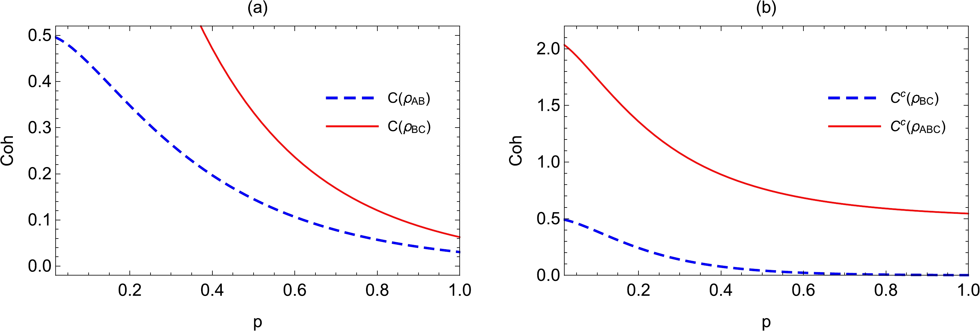
Figure 3. (color online) Bipartite coherence
$ C(\rho_{AB}) $ ,$ C(\rho_{BC}) $ , correlated coherence$ C^{c}(\rho_{BC}) $ , and$ C^{c}(\rho_{ABC}) $ of the GHZ state as a function of the curvature parameter p for a fixed$ \nu=3/2 $ . -
In this section, we assume that Alice, Bob, and Charlie initially share the W state
$ \begin{split} |W\rangle=\,& \frac{1}{\sqrt{3}}[|0\rangle_{A, {\rm{BD}}_{1}}|0\rangle_{B, {\rm{BD}}_{2}}|1\rangle_{C, {\rm{BD}}_{3}} +|0\rangle_{A, {\rm{BD}}_{1}}|1\rangle_{B, {\rm{BD}}_{2}}|0\rangle_{C, {\rm{BD}}_{3}} \\ & + |1\rangle_{A, {\rm{BD}}_{1}}|0\rangle_{B, {\rm{BD}}_{2}}|0\rangle_{C, {\rm{BD}}_{3}}].\\[-1pt] \end{split} $

(42) Following the treatment for the GHZ state, the W state becomes
$ \begin{aligned}[b] |W\rangle_{AB\bar{B}C\bar{C}}=\;&\frac{(1-|\gamma_{p}|^{2})^{\frac{3}{2}}}{\sqrt{6}}\sum\limits_{n,m=0}^{\infty}\gamma_{p}^{n}\gamma_{p}^{m}\big[\sqrt{m+1}|0\rangle_{A} |n\rangle_{B} |n\rangle_{\bar{B}}(| m\rangle_{C}|m+1\rangle_{\bar{C}}\\&+|(m+1)\rangle_{C}|m\rangle_{\bar{C}} )+\sqrt{n+1}|0\rangle_{A}(|n\rangle_{B}|n+1\rangle_{\bar{B}}+|n+1\rangle_{B}+|n\rangle_{\bar{B}})\\ &\otimes|m\rangle_{C}|m\rangle_{\bar{C}}+\sqrt{2}(1-|\gamma_{p}|^{2})^{-\frac{1}{2}}|1\rangle_{A} |n\rangle_{B}|n\rangle_{\bar{B}} |m\rangle_{C}|m\rangle_{\bar{C}}\big]. \end{aligned} $

(43) The reduced density matrix after tracing over the modes
$ \bar{B} $ and$ \bar{C} $ can be expressed as$ \rho_{ABC}=\frac{1}{3}\sum\limits_{n,m=0}^{\infty}\gamma_{p}^{2n}\gamma_{p}^{2m}\rho_{n,m} $

(44) $ \begin{aligned} \rho_{n,m}=&|0\rangle_{A}\langle0|\otimes(1-|\gamma_{p}|^{2})|n\rangle_{B}\langle n| \otimes \frac{(1-|\gamma_{p}|^{2})^{2}}{2}[(m+1)(|m\rangle_{C}\langle m|+|m+1\rangle_{C}\langle m+1|) +\sqrt{m+2}\sqrt{m+1}(\gamma_{p}^{*}|m\rangle_{C}\langle m+2|\\ &+\gamma_{p}|m+2\rangle_{C}\langle m|)] + |0\rangle_{A}\langle0|\otimes\frac{(1-|\gamma_{p}|^{2})^{2}}{2} [(n+1)(|n\rangle_{B}\langle n|+|n+1\rangle_{B}\langle n+1|)+\sqrt{n+1}\sqrt{n+2} (\gamma_{p}^{*}|n\rangle_{B}\\ & \langle n+2|+\gamma_{p}|n+2\rangle_{B}\langle n|)](1-|\gamma_{p}|^{2})\otimes|m\rangle_{C}\langle m| + [|0\rangle_{A}\langle0|\otimes\frac{(1-|\gamma_{p}|^{2})^{\frac{3}{2}}}{\sqrt{2}}\sqrt{n+1}[|n\rangle_{B}\langle n+1|+\gamma_{p}|n+1\rangle_{B}\langle n|]\\ &\otimes\frac{(1-|\gamma_{p}|^{2})^{\frac{3}{2}}}{\sqrt{2}}\sqrt{m+1}[\gamma_{p}^{*}|m\rangle_{C}\langle m+1|+|m+1\rangle_{C}\langle m|]+h.c.] +[|0\rangle_{A}\langle1||n\rangle_{B}\langle n|\otimes\frac{(1-|\gamma_{p}|^{2})^{\frac{3}{2}}}{\sqrt{2}}\sqrt{m+1}[\gamma_{p}^{*}|m\rangle_{C}\\ &\langle m+1|+|m+1\rangle_{C}\langle m|]+h.c.]+[|1\rangle_{A}\langle0| \otimes\frac{(1-|\gamma_{p}|^{2})^{\frac{3}{2}}}{\sqrt{2}}\sqrt{n+1}[|n\rangle_{B}\langle n+1| +\gamma_{p}|n+1\rangle_{B}\langle n|]\otimes|m\rangle_{C}\langle m|+h.c.] \\ &+ (1-|\gamma_{p}|^{2})^{2}{[|1\rangle_{A}\langle1||n\rangle_{B}\langle n||m\rangle_{C}\langle m|]}. \end{aligned} $

(45) Employing Eq. (27), the coherence of the W state becomes
$ \begin{aligned}[b] C(\rho_{ABC})=&\frac{1}{3}\{2(1-|\gamma_{p}|^{2})^{2}\sum\limits_{n=0}^{\infty}|\gamma_{p}|^{2n+1}\sqrt{n+2}\sqrt{n+1}\\ &+2\sqrt{2}(1-|\gamma_{p}|^{2})^{\frac{3}{2}}\sum\limits_{m=0}^{\infty}|\gamma_{p}|^{2m}\sqrt{m+1}(|\gamma_{p}|+1)\\ &+(1-|\gamma_{p}|^{2})^{3}[\sum\limits_{m=0}^{\infty}|\gamma_{p}|^{2m}\sqrt{m+1}(|\gamma_{p}|+1)]^{2}\}. \end{aligned} $

(46) As shown in Fig. 4, quantum coherence of the W state decreases monotonically with an increase in the curvature parameter p, which indicates that quantum coherence increases monotonically with increasing curvature. From Fig. 4, we also find that quantum coherence of the W state is most severely affected by the curvature effect of de Sitter space for
$ \nu\rightarrow1/2 $ (conformally coupled massless limit) and$ \nu\rightarrow3/2 $ (minimally coupled massless limit). In addition, quantum coherence of the W state is larger than that of the GHZ state, which means that quantum coherence of the W state is more suitable for processing quantum information tasks in the multiverse.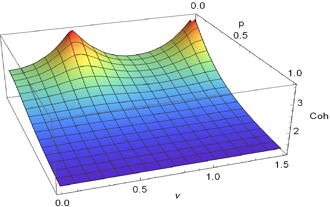
Figure 4. (color online) Quantum coherence
$ C(\rho_{ABC}) $ of the W state as a function of the mass parameter ν and curvature parameter p.We obtain the density matrix
$ \rho_{BC} $ ,$ \rho_{AC} $ , and$ \rho_{AB} $ after tracing over the modes A, B, and C from the state$ \rho_{ABC} $ , respectively.$ \begin{split} \qquad\;\; \rho_{BC}=&\frac{1}{3}[[(1-|\gamma_{p}|^{2})\sum\limits_{n=0}^{\infty}\gamma_{p}^{2n}|n\rangle_{B}\langle n|\otimes\frac{(1-|\gamma_{p}|^{2})^{2}}{2}\sum\limits_{m=0}^{\infty}\gamma_{p}^{2m}[(m+1)(|m\rangle_{C}\langle m|+|m+1\rangle_{C}\langle m+1|)+\sqrt{m+1}\sqrt{m+2}\\ &(\gamma_{p}|m+2\rangle_{C} \langle m|+\gamma_{p}^{*}|m\rangle_{C}\langle m+2|)]+h.c.] +[\frac{(1-|\gamma_{p}|^{2})^{\frac{3}{2}}}{\sqrt{2}}\sum\limits_{n=0}^{\infty}\gamma_{p}^{2n}\sqrt{n+1} (|n\rangle_{B}\langle n+1|+\gamma_{p}|n+1\rangle_{B}\langle n|) \otimes \frac{(1-|\gamma_{p}|^{2})^{\frac{3}{2}}}{\sqrt{2}}\\ &\sum\limits_{m=0}^{\infty}\gamma_{p}^{2m}\sqrt{m+1} (|m+1\rangle_{C}\langle m|+\gamma_{p}^{*}|m\rangle_{C}\langle m+1|)+ h.c.] +(1-|\gamma_{p}|^{2})\sum\limits_{n=0}^{\infty}\gamma_{p}^{2n}|n\rangle_{B}\langle n|\otimes(1-|\gamma_{p}|^{2})\sum\limits_{m=0}^{\infty}\gamma_{p}^{2m}|m\rangle_{C}\langle m|], \end{split} $

(47) $ \begin{split} \qquad\; \rho_{AC}=&\frac{1}{3}[|0\rangle_{A}\langle0|\otimes\frac{(1-|\gamma_{p}|^{2})^{2}}{2}\sum\limits_{m=0}^{\infty}\gamma_{p}^{2m}[(m+1)(|m\rangle_{B}\langle m|+|m+1\rangle_{B}\langle m+1|) +\sqrt{m+1}\sqrt{m+2}(\gamma_{p}|m+2\rangle_{B} \langle m|+\gamma_{p}^{*}|m\rangle_{B}\langle m+2|)]\\ &+|0\rangle_{A}\langle1| \otimes\frac{(1-|\gamma_{p}|^{2})^{\frac{3}{2}}}{\sqrt{2}}\sum\limits_{m=0}^{\infty}\gamma_{p}^{2m}\sqrt{m+1} (|m+1\rangle_{B}\langle m|+\gamma_{p}^{*}|m\rangle_{B}\langle m+1|) +|1\rangle_{A}\langle0|\otimes\frac{(1-|\gamma_{p}|^{2})^{\frac{3}{2}}}{\sqrt{2}}\sum\limits_{m=0}^{\infty}\gamma_{p}^{2m}\sqrt{m+1} (|m+1\rangle_{B}\langle m|\\ &+\gamma_{p}^{*}|m\rangle_{B}\langle m+1|) +|0\rangle_{A}\langle0|\otimes (1-|\gamma_{p}|^{2})\sum\limits_{m=0}^{\infty}\gamma_{p}^{2m}|m\rangle_{B}\langle m|+|1\rangle_{A}\langle1|\otimes(1-|\gamma_{p}|^{2})\sum\limits_{m=0}^{\infty}\gamma_{p}^{2m}|m\rangle_{B}\langle m|], \end{split} $

(48) $ \begin{split} \qquad\;\rho_{AB}=&\frac{1}{3}[|0\rangle_{A}\langle0|\otimes\frac{(1-|\gamma_{p}|^{2})^{2}}{2}\sum\limits_{m=0}^{\infty}\gamma_{p}^{2m}[(m+1)(|m\rangle_{C}\langle m|+|m+1\rangle_{C}\langle m+1|) +\sqrt{m+1}\sqrt{m+2}(\gamma_{p}|m+2\rangle_{C} \langle m|+\gamma_{p}^{*}|m\rangle_{C}\langle m+2|)]\\ &+|0\rangle_{A}\langle1| \otimes\frac{(1-|\gamma_{p}|^{2})^{\frac{3}{2}}}{\sqrt{2}}\sum\limits_{m=0}^{\infty}\gamma_{p}^{2m}\sqrt{m+1} (|m+1\rangle_{C}\langle m|+\gamma_{p}^{*}|m\rangle_{C}\langle m+1|)+|1\rangle_{A}\langle0|\otimes\frac{(1-|\gamma_{p}|^{2})^{\frac{3}{2}}}{\sqrt{2}}\\ &\sum\limits_{m=0}^{\infty}\gamma_{p}^{2m}\sqrt{m+1} (|m+1\rangle_{C}\langle m|+\gamma_{p}^{*}|m\rangle_{C}\langle m+1|)+|0\rangle_{A}\langle0|\otimes (1-|\gamma_{p}|^{2})\sum\limits_{m=0}^{\infty}\gamma_{p}^{2m}|m\rangle_{C}\langle m|+|1\rangle_{A}\\ &\langle1|\otimes(1-|\gamma_{p}|^{2})\sum\limits_{m=0}^{\infty}\gamma_{p}^{2m}|m\rangle_{C}\langle m|]. \end{split} $

(49) Using Eq. (27), we obtain the bipartite coherence as
$ \begin{aligned}[b] C(\rho_{BC})=&\frac{1}{3}\{2(1-|\gamma_{p}|^{2})^{2}\sum\limits_{n=0}^{\infty}\sqrt{n+1}\sqrt{n+2}|\gamma_{p}|^{2n+1}\\ &+ (1-|\gamma_{p}|^{2})^{3}[\sum\limits_{n=0}^{\infty}|\gamma_{p}|^{2n}\sqrt{n+1}(|\gamma_{p}|+1)]^{2}\}, \end{aligned} $

(50) $ \begin{split} C(\rho_{AC})=&C(\rho_{AB})=\frac{1}{3}[(1-|\gamma_{p}|^{2})^{2}\sum\limits_{n=0}^{\infty}\sqrt{n+1}\sqrt{n+2}|\\ & \times \gamma_{p}|^{2n+1} +\sqrt{2}(1-|\gamma_{p}|^{2})^{\frac{3}{2}}\sum\limits_{n=0}^{\infty}|\gamma_{p}|^{2n}\sqrt{n+1}\\ & \times (1+|\gamma_{p}|)].\\[-1pt] \end{split} $

(51) Similarly, we obtain the density matrices
$ \rho_{A}, \rho_{B} $ , and$ \rho_{C} $ of the single particle system as$ \rho_{A}=\frac{1}{3}(2|0\rangle_{A}\langle0|+|1\rangle_{A}\langle1|), $

(52) $ \begin{aligned}[b] \rho_{B}=&\frac{1}{3}[2(1-|\gamma_{p}|^{2})\sum\limits_{m=0}^{\infty}\gamma_{p}^{2m}|m\rangle_{B}\langle m|+\frac{(1-|\gamma_{p}|^{2})^{2}}{2}\\ & \sum\limits_{m=0}^{\infty}\gamma_{p}^{2m}[(m+1)(|m\rangle_{B}\langle m|+|m+1\rangle_{B}\langle m+1|)\\ &+\sqrt{m+1}\sqrt{m+2}(\gamma_{p}|m+2\rangle_{B} \langle m|+\gamma_{p}^{*}|m\rangle_{B}\langle m+2|)]], \end{aligned} $

(53) $ \begin{aligned}[b] \rho_{C}=&\frac{1}{3}v[2(1-|\gamma_{p}|^{2})\sum\limits_{m=0}^{\infty}\gamma_{p}^{2m}|m\rangle_{C}\langle m|+\frac{(1-|\gamma_{p}|^{2})^{2}}{2}\\ &\sum\limits_{m=0}^{\infty}\gamma_{p}^{2m}[(m+1)(|m\rangle_{C}\langle m|+|m+1\rangle_{C}\langle m+1|)\\ &+\sqrt{m+1}\sqrt{m+2}(\gamma_{p}|m+2\rangle_{C} \langle m|+\gamma_{p}^{*}|m\rangle_{C}\langle m+2|)]]. \end{aligned} $

(54) The corresponding single particle coherence reads as
$ C(\rho_{A})=0, $

(55) $ C(\rho_{B})=C(\rho_{C})= \frac{(1-|\gamma_{p}|^{2})^{2}}{3}\sum\limits_{n=0}^{\infty}\sqrt{n+1}\sqrt{n+2}|\gamma_{p}|^{2n+1}. $

(56) According to Eq. (36), we can obtain the correlated coherence as
$ \begin{aligned}[b] C^{c}(\rho_{ABC})=&\frac{1}{3}\{2\sqrt{2}(1-|\gamma_{p}|^{2})^{\frac{3}{2}}\sum\limits_{m=0}^{\infty}|\gamma_{p}|^{2m}\sqrt{m+1}(|\gamma_{p}|+1)\\ &+(1-|\gamma_{p}|^{2})^{3}[\sum\limits_{m=0}^{\infty}|\gamma_{p}|^{2m}\sqrt{m+1}(|\gamma_{p}|+1)]^{2}\}, \end{aligned} $

(57) $ \begin{aligned}[b] C^{c}(\rho_{AB})=\,& C^{c}(\rho_{AC})= \frac{\sqrt{2}(1-|\gamma_{p}|^{2})^{\frac{3}{2}}}{3} \sum\limits_{n=0}^{\infty}|\gamma_{p}|^{2n}\sqrt{n+1}(|\gamma_{p}|+1), \end{aligned} $

(58) $ C^{c}(\rho_{BC})= \frac{(1-|\gamma_{p}|^{2})^{3}}{3}[\sum\limits_{n=0}^{\infty}|\gamma_{p}|^{2n}\sqrt{n+1}(|\gamma_{p}|+1)]^{2}. $

(59) As shown in Fig. 5, the properties of the single particle coherence
$ C(\rho_{A}) $ and$ C(\rho_{B}) $ , bipartite coherence$ C(\rho_{BC}) $ and$ C(\rho_{AB}) $ , and correlated coherence$ C^{c}(\rho_{AB}) $ ,$ C^{c}(\rho_{BC}) $ , and$ C^{c}(\rho_{ABC}) $ in the W state are similar to those in the GHZ state.
Figure 5. (color online) Single particle coherence
$ C(\rho_{A}) $ and$ C(\rho_{B}) $ , bipartite coherence$ C(\rho_{BC}) $ and$ C(\rho_{AB}) $ , and correlated coherence$ C^{c}(\rho_{AB}) $ ,$ C^{c}(\rho_{BC}) $ , and$ C^{c}(\rho_{ABC}) $ of the W state as a function of the curvature parameter p for a fixed$ \nu=3/2 $ .The relationship of quantum coherence for the W state is still unclear in the multiverse. Through direct calculation, we obtain a distribution relationship between the correlated coherence of the tripartite W state as
$ C^{c}(\rho_{ABC})= C^{c}(\rho_{AB})+C^{c}(\rho_{BC})+C^{c}(\rho_{AC}). $

(60) From Eq. (60), we find that the correlated coherence of the W state exists essentially in the form of bipartite correlated coherence, showing that the correlated coherence of the tripartite system is equal to the sum of all the bipartite correlated coherence in the multiverse. In addition, Eqs. (18) and (19) are very similar to Eqs. (14) and (16) for
$ q_R=1/\sqrt{2} $ in reference [55]. Therefore, the properties of multipartite coherence in de Sitter space are similar to those beyond the single-mode approximation in Rindler spacetime. -
In this section, we discuss the extension of the tripartite systems to N-partite systems (N
$ \geq 3 $ ). The N-partite GHZ and N-partite W states can be written as$ \begin{split} |GHZ\rangle_{123\cdot\cdot\cdot N}=\;& \frac{1}{\sqrt{2}}(|0\rangle_{{\rm{BD}}, 1}|0\rangle_{{\rm{BD}}, 2}...|0\rangle_{{\rm{BD}}, (N-1)}|0\rangle_{{\rm{BD}}, N} \\ &+ |1\rangle_{{\rm{BD}}, 1}|1\rangle_{{\rm{BD}}, 2}...|1\rangle_{{\rm{BD}}, (N-1)}|1\rangle_{{\rm{BD}}, N}), \end{split} $

(61) $ \begin{aligned}[b] |W\rangle_{123\cdot\cdot\cdot N}=&\frac{1}{N}(|1\rangle_{{\rm{BD}}, 1}|0\rangle_{{\rm{BD}}, 2}..|0\rangle_{{\rm{BD}}, (N-1)}|0\rangle_{{\rm{BD}}, N}\\ &+|0_{{\rm{BD}}, 1}|1\rangle_{{\rm{BD}}, 2}...|0_{{\rm{BD}}, (N-1)}|0\rangle_{{\rm{BD}}, N}+\cdot\cdot\cdot\\ &+|0_{{\rm{BD}},1}|0\rangle_{{\rm{BD}}, 2}...|0\rangle_{{\rm{BD}}, (N-1)}|1\rangle_{{\rm{BD}}, N}), \end{aligned} $

(62) where the mode i (
$ i=1, 2, ..., N $ )) is observed by observer$ O_i $ in de Sitter space$ {\rm{BD}}_{i} $ . Now, we assume that n ($ 2\leq n\leq N-1 $ ) observers are in the different L regions of the expanded de Sitter spaces and$ N-n $ observers are in the global charts of the other de Sitter spaces. Through a series of calculations, we obtain N-partite coherence of the GHZ and W states as$ \begin{split} \qquad C({\rm GHZ})=&\frac{1}{2}\bigg\{2\bigg[\frac{(1 - |\gamma_{p}|^{2})^{\frac{3}{2}}}{\sqrt{2}}\sum\limits_{m=0}^{\infty} |\gamma_{p}|^{2m}\sqrt{m + 1}(|\gamma_{p}|+1)\bigg]^{n}\\ &+\bigg[1+(1-|\gamma_{p}|^{2})^{2}\sum\limits_{m=0}^{\infty} |\gamma_{p}|^{2m+1}\\ & \sqrt{m+1}\sqrt{m+2}\bigg]^{n}-1\bigg\}, \end{split} $

(63) $ \begin{aligned}[b] C(W)=&\frac{1}{N}\bigg\{n(1-|\gamma_{p}|^{2})^{2}\sum\limits_{m=0}^{\infty}\sqrt{m+1}\sqrt{m+2}|\gamma_{p}|^{2m+1}\\ & +2n(N-n)\frac{(1-|\gamma_{p}|^{2})^{\frac{3}{2}}}{\sqrt{2}}\sum\limits_{m=0}^{\infty} |\gamma_{p}|^{2m}\sqrt{m+1}\\ &(|\gamma_{p}|+1)+n(n-1)[\frac{(1-|\gamma_{p}|^{2})^{\frac{3}{2}}}{\sqrt{2}}\sum\limits_{m=0}^{\infty} |\gamma_{p}|^{2m}\\ &\sqrt{m+1}(|\gamma_{p}|+1)]^{2}+(N-n)(N-n-1)\bigg\}. \end{aligned} $

(64) After tedious but straightforward calculations, the correlated coherence of the GHZ and W states reads as
$ \begin{split} C^{c}( GHZ)=&\frac{1}{2}\bigg\{2\bigg[\frac{(1-|\gamma_{p}|^{2})^{\frac{3}{2}}}{\sqrt{2}}\sum\limits_{m=0}^{\infty} |\gamma_{p}|^{2m}\sqrt{m+1}(|\gamma_{p}|+1)\bigg]^{n}\\&+\bigg[ 1+(1-|\gamma_{p}|^{2})^{2}\sum\limits_{m=0}^{\infty} |\gamma_{p}|^{2m+1}\sqrt{m+1}\sqrt{m+2}\bigg]^{n}-1\\&-n(1-|\gamma_{p}|^{2})^{2}\sum\limits_{m=0}^{\infty} |\gamma_{p}|^{2m+1}\sqrt{m+1}\sqrt{m+2}\bigg\}, \end{split} $

(65) $ \begin{split} C^{c}(W)=&\frac{1}{N}\bigg[2n(N-n)\frac{(1-|\gamma_{p}|^{2})^{\frac{3}{2}}}{\sqrt{2}}\sum\limits_{m=0}^{\infty} |\gamma_{p}|^{2m}\sqrt{m+1}(|\gamma_{p}|+1)\\& + n(n-1)[\frac{(1-|\gamma_{p}|^{2})^{\frac{3}{2}}}{\sqrt{2}}\sum\limits_{m=0}^{\infty} |\gamma_{p}|^{2m}\sqrt{m+1}(|\gamma_{p}|+1)]^{2}\\& +(N-n)(N-n-1)\bigg]. \end{split} $

(66) As shown in Eqs. (63)−(66), N-partite (correlated) coherence of the GHZ state depends only on the n observers who are in the different L regions of the expanded de Sitter spaces, whereas N-partite (correlated) coherence of the W state depends not only on the n observers but also on the initial N observers.
From Fig. 6, we find that the curvature effect enhances N-partite (correlated) coherence. Therefore, the curvature effect is beneficial to N-partite (correlated) coherence in the multiverse consisting of many de Sitter spaces. As shown in Fig. 7 (a)−(b), N-partite (correlated) coherence of the GHZ state increases monotonically with increasing n for any curvature parameter p. Fig. 7 (c)−(d) show that with an increase in n, N-partite (correlated) coherence of the W state increases monotonically for a smaller curvature parameter p, whereas it decreases monotonically for a larger curvature parameter p in the multiverse. From Fig. 8, we find that N-partite (correlated) coherence of the W state increases monotonically with increasing N for any p and n, whereas N-partite (correlated) coherence of the GHZ state is independent of N. We can also see that N-partite (correlated) coherence of the W state increases or decreases monotonically with increasing n depending on the curvature parameter p.
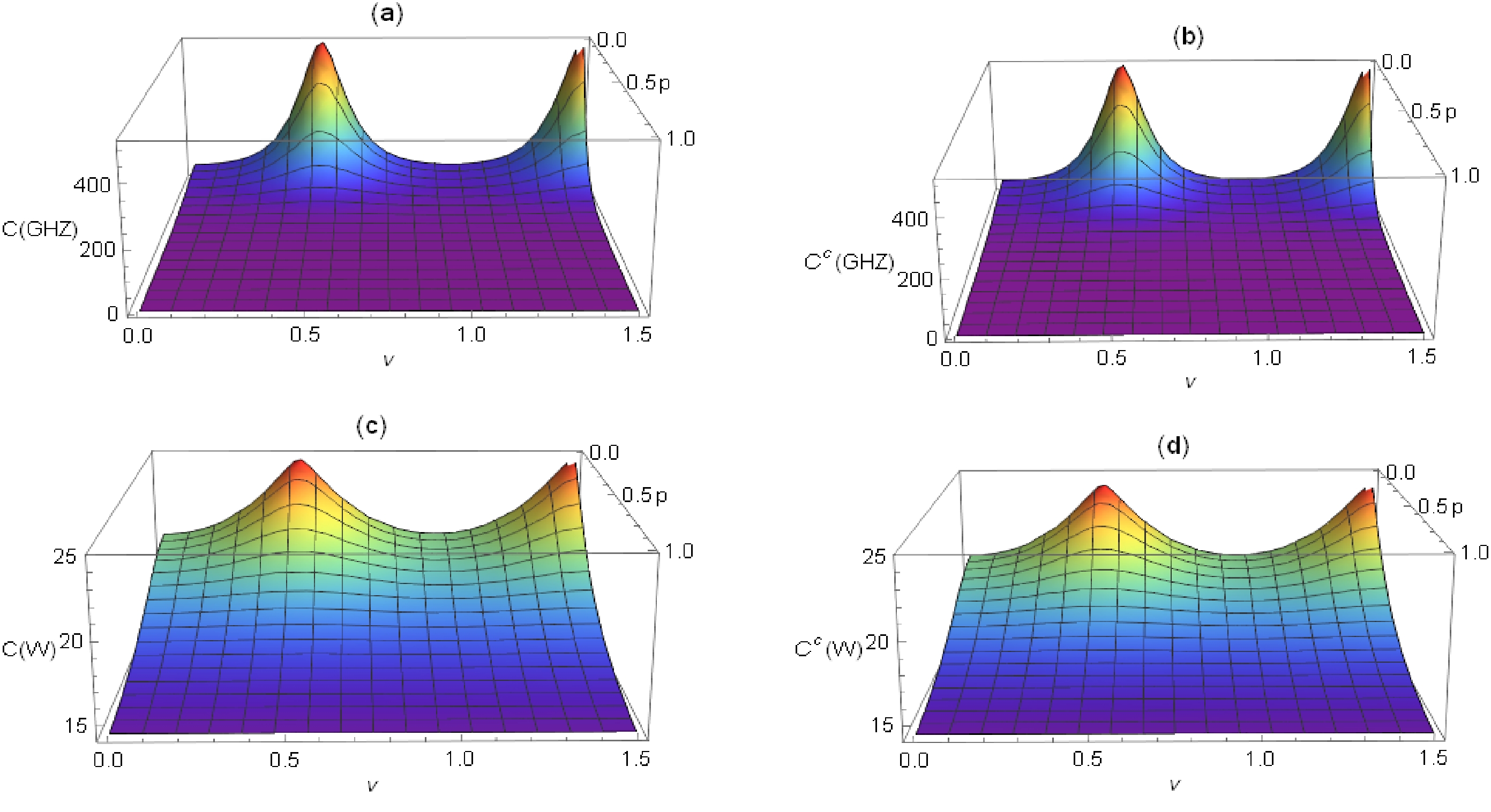
Figure 6. (color online) N-partite coherence and correlated coherence of the GHZ and W states as functions of the mass parameter ν and curvature parameter p for fixed n=10 and N=20.

Figure 7. (color online) N-partite coherence and correlated coherence of the GHZ and W states as functions of the curvature parameter p for fixed
$ \nu= 3/2 $ , N = 20 and different n.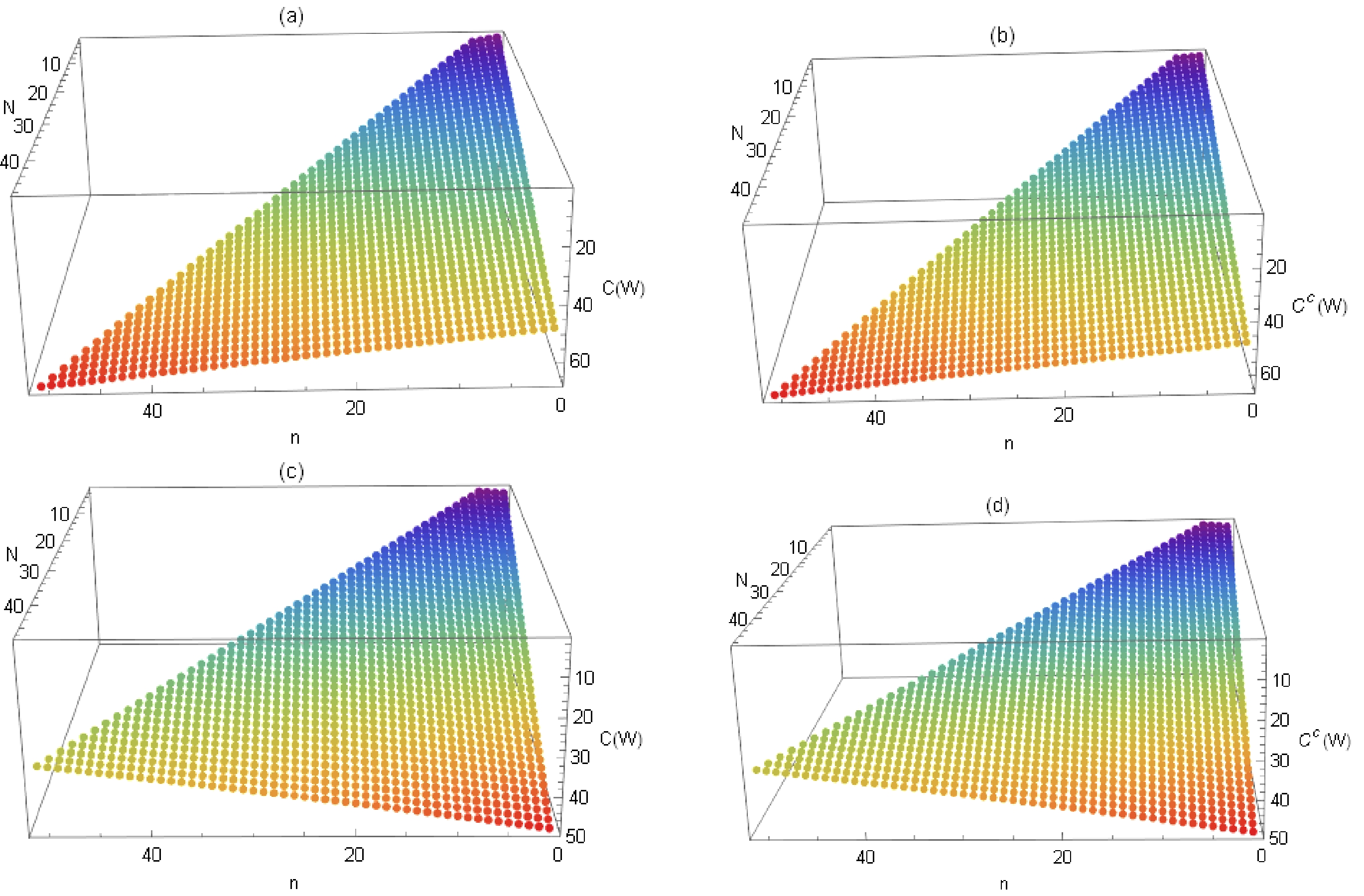
Figure 8. (color online) N-partite coherence and correlated coherence of the W state as functions of n and N for
$ p=0.1 $ (a) and (b),$ p=0.6 $ (c) and (d). The parameter ν is fixed as$ \nu=3/2 $ .Next, we study the distribution relationship of coherence for N-partite systems in the multiverse. For the N-partite W state, the distribution relationship of the correlated coherence can be written as
$ \begin{aligned}[b] & \frac{n(n-1)}{2}C^{c}(\rho_{O} \rho_{O} )+n(N-n)C^{c}(\rho_{O}\rho_{X} )\\ &\quad+\frac{(N-n)(N-n-1)}{2} C^{c}(\rho_{X}\rho_{X})=C^{c}(W). \end{aligned} $

(67) Here,
$ C^{c}(\rho_{O}\rho_{O} )=\frac{2}{N}[\frac{(1-|\gamma_{p}|^{2})^{\frac{3}{2}}}{\sqrt{2}}\sum\limits_{m=0}^{\infty} |\gamma_{p}|^{2m}\sqrt{m+1}(|\gamma_{p}|+1)]^{2} $

denotes the bipartite correlated coherence of the modes corresponding to two observers in the L regions of the expanded de Sitter spaces;
$ C^{c}(\rho_{O}\rho_{X})= \frac{2}{N}\frac{(1-|\gamma_{p}|^{2})^{\frac{3}{2}}}{\sqrt{2}}\sum\limits_{m=0}^{\infty} |\gamma_{p}|^{2m}\sqrt{m+1}(|\gamma_{p}|+1) $

denotes the bipartite correlated coherence of the modes corresponding to two observers who are in the L region of the expanded de Sitter space and the global chart of de Sitter space, respectively;
$ C^{c}(\rho_{X}\rho_{X})= {2}/{N} $ denotes the bipartite correlated coherence of the modes corresponding to two observers in the global chart of de Sitter spaces. From Eq. (67), we find that the total correlated coherence of the N-partite W state is equal to the sum of all bipartite correlated coherence in the multiverse. -
The curvature effect on quantum coherence of tripartite GHZ and W states in the multiverse is investigated. We show that tripartite coherence increases with curvature, indicating that the curvature effect is beneficial to quantum coherence in the multiverse. However, with increasing curvature, quantum entanglement gradually vanishes and quantum discord gradually decreases to a fixed value at the limit of infinite curvature in de Sitter space [25–28]. We find that quantum coherence of the GHZ and W states is sensitive to the curvature effect in the limit of conformal and massless scalar fields. Interestingly, the curvature effect can generate bipartite quantum coherence and single-partite quantum coherence. We obtain a distribution relationship of correlated coherence for the W state in the multiverse. In other words, tripartite correlated coherence of the W state is equal to the sum of all bipartite correlated coherence.
We extend the investigation from tripartite systems to N-partite systems in the multiverse. Unlike tripartite coherence, N-partite coherence of the W state depends not only on the curvature and mass parameters, but also on the n particles in the L regions of the de Sitter spaces and the initial N particles. However, N-partite coherence of the GHZ state is independent of N. We find that with increasing n, N-partite coherence of the GHZ state increases monotonically for any curvature, whereas N-partite coherence of the W state increases or decreases monotonically, depending on the curvature. We extend the tripartite distribution relationship to the N-partite distribution relationship. This indicates that the total correlated coherence of the N-partite W state is essentially a bipartite type. Based on the above arguments, we expect that multipartite coherence will be able to provide some evidence for the existence of the multiverse.
Curvature-enhanced multipartite coherence in the multiverse
- Received Date: 2024-01-19
- Available Online: 2024-07-15
Abstract: Here, we study the quantum coherence of N-partite Greenberger-Horne-Zeilinger (GHZ) and W states in the multiverse consisting of N causally disconnected de Sitter spaces. Interestingly, N-partite coherence increases monotonically with curvature, whereas the curvature effect destroys quantum entanglement and discord, indicating that the curvature effect is beneficial to quantum coherence and harmful to quantum correlations in the multiverse. We find that with an increase in n expanding de Sitter spaces, the N-partite coherence of the GHZ state increases monotonically for any curvature, whereas the quantum coherence of the W state decreases or increases monotonically depending on the curvature. We find a distribution relationship, which indicates that the correlated coherence of the N-partite W state is equal to the sum of all bipartite correlated coherence in the multiverse. Multipartite coherence exhibits unique properties in the multiverse, suggesting that it may provide some evidence for the existence of the multiverse.


 DownLoad: