


 Abstract
 HTML
HTML Reference
 Related
 PDF
PDF


-
The
$ (g-2)_{\mu} $ anomaly is a longstanding puzzle in the standard model (SM) of elementary particle physics. It was first announced by the BNL E821 experiment [1]. Last year, the FNAL muon$ g-2 $ experiment revealed increased deviation from the SM prediction [2]. When combining the BNL and FNAL data, the averaged result is$ a_{\mu}^{ \mathrm{Exp}}=116592061(41)\times10^{-11} $ . Compared to the SM prediction$ a_{\mu}^{ \mathrm{SM}}=116591810(43)\times10^{-11} $ [3−23], the deviation is$ \Delta a_{\mu}\equiv a_{\mu}^{ \mathrm{Exp}}-a_{\mu}^{ \mathrm{SM}}=(251\pm59)\times10^{-11} $ , which shows a$ 4.2\sigma $ discrepancy. Many new physics models were proposed to explain the anomaly [24−29].For the mediators with mass above the TeV level, the chiral enhancements are required, which can appear when left-handed and right-handed muons couple to a heavy fermion simultaneously. In the new lepton extended models [30−33], the chiral enhancements originate from the large lepton mass. The LQ models are an alternative choice [34−40], in which the chiral enhancements originate from the large quark mass. For the minimal LQ models, there are scalar LQs
$ R_2/S_1 $ with top quark chiral enhancement and vector LQs$ V_2/U_1 $ with bottom quark chiral enhancement. The LQ can connect the lepton sector and quark sector. On the other hand, the VLQ naturally occurs in many new physics models and is free of quantum anomaly. It can mix with SM quarks and provide new source of CP violation. Hence, the LQ and VLQ extended models can lead to interesting flavour physics in both the lepton sector and quark sector. In our previous study [41], we investigated the scalar LQ and VLQ1 extended models with top and top partner chiral enhancements. In this study, we investigate the scalar LQ and VLQ extended models, which can produce the bottom partner chiral enhancements. This paper is complementary to our previous paper [41]. Moreover, the top partner and bottom partner lead to different collider signatures.In Sec. II, we introduce the models and show the related interactions. Then, we derive the new physics contributions to
$ (g-2)_{\mu} $ and perform the numerical analysis in Sec. III. In Sec. IV, we discuss the possible collider phenomenology. Finally, we present a summary and conclusions in Sec. V. -
Typically, there are six types of scalar LQs [35], which carry a conserved quantum number
$F\equiv 3B+ L$ . Here, B and L are the baryon and lepton numbers. As for the VLQs, there are seven typical representations [42]. In Table 1, we list their representations and labels.$S U(3)_C\times S U(2)_L\times U(1)_Y$ 

representationlabel F $S U(3)_C\times S U(2)_L\times U(1)_Y$ 

representationlabel $ (\bar{3},3,1/3) $ 

$ S_3 $ 

$ -2 $ 

$(3,1,2/3)$ 

$T_{L,R}$ 

$ (3,2,7/6) $ 

$ R_2 $ 

0 $(3,1,-1/3)$ 

$B_{L,R}$ 

$ (3,2,1/6) $ 

$ \widetilde{R}_2 $ 

0 $(3,2,7/6)$ 

$(X,T)_{L,R}$ 

$ (\bar{3},1,4/3) $ 

$ \widetilde{S}_1 $ 

$ -2 $ 

$(3,2,1/6)$ 

$(T,B)_{L,R}$ 

$(3,2,-5/6)$ 

$(B,Y)_{L,R}$ 

$ (\bar{3},1,1/3) $ 

$ S_1 $ 

$ -2 $ 

$(3,3,2/3)$ 

$(X,T,B)_{L,R}$ 

$ (\bar{3},1,-2/3) $ 

$ \bar{S}_1 $ 

$ -2 $ 

$(3,3,-1/3)$ 

$(T,B,Y)_{L,R}$ 

Table 1. Scalar LQ (left) and VLQ (right) representations.
For the six types of scalar LQs and seven types of VLQs, there can be a total of 42 combinations, which are named "
$ \mathrm{LQ}+ \mathrm{VLQ} $ " for convenience. Only 17 of them can lead to the chiral enhancements. In Table 2, we list these models that feature the chiral enhancements. The contributons in the four models$ R_2+B_{L,R}/(B,Y)_{L,R} $ and$ S_1+B_{L,R}/(B,Y)_{L,R} $ are almost the same as those in the minimal$ R_2 $ and$ S_1 $ models. There are nine models$ R_2+T_{L,R}/(X,T)_{L,R}/(T,B)_{L,R}/(T,B,Y)_{L,R} $ and$S_1+T_{L,R}/ (X,T)_{L,R}/(T,B)_{L,R}/(X,T,B)_{L,R}/(T,B,Y)_{L,R}$ , which produce the top and top partner chiral enhancements. For the two models$ R_2/S_3+(X,T,B)_{L,R} $ , there are top, top partner, bottom, and bottom partner chiral enhancements at the same time. The models including T quarks were investigated in our previous work [41]. Here, we will study the pure bottom partner chirally enhanced models$\tilde{R}_2/\tilde{S}_1+ (B,Y)_{L,R}$ .Model Chiral enhancement $ R_2 $ 

$ m_t/m_{\mu} $ 

$ S_1 $ 

$ m_t/m_{\mu} $ 

$ R_2+B_{L,R}/(B,Y)_{L,R} $ 

$ m_t/m_{\mu} $ 

$ S_1+B_{L,R}/(B,Y)_{L,R} $ 

$ m_t/m_{\mu} $ 

$ R_2+T_{L,R}/(X,T)_{L,R}/(T,B)_{L,R}/(T,B,Y)_{L,R} $ 

$ m_t/m_{\mu},m_T/m_{\mu} $ 

$ S_1+T_{L,R}/(X,T)_{L,R}/(T,B)_{L,R}/(X,T,B)_{L,R}/(T,B,Y)_{L,R} $ 

$ m_t/m_{\mu},m_T/m_{\mu} $ 

$ R_2+(X,T,B)_{L,R} $ 

$ m_t/m_{\mu},m_T/m_{\mu},m_b/m_{\mu},m_B/m_{\mu} $ 

$ S_3+(X,T,B)_{L,R} $ 

$ m_t/m_{\mu},m_T/m_{\mu},m_b/m_{\mu},m_B/m_{\mu} $ 

$ {\tilde{\bf R}_2+\bf(B,Y)_{L,R}} $ 

$ m_b/m_{\mu},m_B/m_{\mu} $ 

$ {\tilde{\bf S}_1+\bf(B,Y)_{L,R}} $ 

$ m_b/m_{\mu},m_B/m_{\mu} $ 

Table 2. Chiral enhancements in the minimal LQ and LQ+VLQ models.
-
Let us start with the
$ (B,Y)_{L,R} $ related Higgs Yukawa interactions. In the gauge eigenstates, there are two interactions$ \overline{Q_L}^id_R^j\phi $ and$ (\overline{B_L},\overline{Y_L})d_R^j\tilde{\phi} $ and the mass term$ -M_B(\bar{B}B+\bar{Y}Y) $ . Here, we define the SM Higgs doublet$\tilde{\phi}\equiv {\rm i}\sigma^2\phi^{\ast}$ with$ \sigma^a(a=1,2,3) $ to be the Pauli matrices. The$ Q_L^i $ and$ d_R^i $ ($ i=1,2,3 $ ) represent the SM quark fields. We can parametrize ϕ as$ [0,(v+h)/{\sqrt{2}}]^T $ in the unitary gauge. After the electroweak symmetry breaking (EWSB), there are mixings between$ d^i $ and B. For simplicity, we only consider mixing between the third generation and B quark. Thus, we can perform the following transformations to rotate b and B quarks into mass eigenstates:$ \begin{aligned}[b]& \left[\begin{array}{c}b_L\\B_L\end{array}\right]\rightarrow \left[\begin{array}{cc}c_L^b& s_L^b\\-s_L^b& c_L^b\end{array}\right] \left[\begin{array}{c}b_L\\B_L\end{array}\right],\\& \left[\begin{array}{c}b_R\\B_R\end{array}\right]\rightarrow \left[\begin{array}{cc}c_R^b& s_R^b\\-s_R^b& c_R^b\end{array}\right] \left[\begin{array}{c}b_R\\B_R\end{array}\right]. \end{aligned} $

(1) Here,
$ s_{L,R}^b $ and$ c_{L,R}^b $ are abbreviations of$ \sin\theta_{L,R}^b $ and$ \cos\theta_{L,R}^b $ , respectively. In fact,$ \theta_L^b $ can be correlated with$ \theta_R^b $ through the relation$ \tan\theta_L^b=m_b\tan\theta_R^b/m_B $ [42]. Here,$ m_b $ and$ m_B $ represent the physical b and B quark masses, respectively. Additionally, the mass of the Y quark is$m_Y=M_B= $ $ \sqrt{m_B^2(c_R^b)^2+m_b^2(s_R^b)^2}$ . Then, we can choose$ m_B $ and$ \theta_R^b $ as the new input parameters. After the transformations in Eq. (1), we obtain the following mass eigenstate Higgs Yukawa interactions:$ \begin{aligned}[b]\mathcal{L}_{\rm H}^{\rm Yukawa}&\supset-\frac{m_b}{v}(c_R^b)^2h\bar{b}b-\frac{m_B}{v}(s_R^b)^2h\bar{B}B\\&-\frac{m_b}{v}s_R^bc_R^bh(\bar{b}_LB_R+\bar{B}_Rb_L)-\frac{m_B}{v}s_R^bc_R^bh(\bar{B}_Lb_R+\bar{b}_RB_L). \end{aligned} $

(2) Note that the Y quark does not interact with Higgs at the tree level.
-
Now, let us label the
$S U(2)_L$ and$ U_Y(1) $ gauge fields as$ W_{\mu}^a $ and$ B_{\mu} $ . Then, the electroweak covariant derivative$ D_{\mu} $ is defined as$\partial_{\mu}-{\rm i}gW_{\mu}^a\sigma^a/2-{\rm i}g^{\prime}Y_qB_{\mu}$ for a doublet and$\partial_{\mu}-{\rm i}g^{\prime}Y_qB_{\mu}$ for a singlet, in which$ Y_q $ is the$ U_Y(1) $ charge of the quark field acted by$ D_{\mu} $ . Thus, the related gauge interactions can be written as$ \overline{Q_L}^iiD_{\mu}\gamma^{\mu}Q_L^i+ \overline{d_R}^iiD_{\mu}\gamma^{\mu}d_R^i+(\overline{B},\overline{Y})iD_{\mu}\gamma^{\mu}(B,Y)^T $ . After the EWSB, the W gauge interactions can be written as$ \mathcal{L}\supset \frac{g}{\sqrt{2}}W_{\mu}^+(\overline{t_L}\gamma^{\mu}b_L+\bar{B}\gamma^{\mu}Y)+\mathrm{h.c.}. $

(3) The Z gauge interactions can be written as
$ \begin{aligned}[b]\mathcal{L}&\supset\frac{g}{c_W}\Bigg[\left(-\frac{1}{2}+\frac{1}{3}s_W^2\right)\overline{b_L}\gamma^{\mu}b_L+\frac{1}{3}s_W^2\overline{b_R}\gamma^{\mu}b_R\\&+\left(\frac{1}{2}+\frac{1}{3}s_W^2\right)\bar{B}\gamma^{\mu}B+\left(-\frac{1}{2}+\frac{4}{3}s_W^2\right)\bar{Y}\gamma^{\mu}Y\Bigg]Z_{\mu}. \end{aligned} $

(4) After the rotations in Eq. (1), we have the mass eigenstate W gauge interactions:
$ \begin{aligned}[b] \mathcal{L}_{\rm BY}^{\rm gauge}&\supset\frac{g}{\sqrt{2}}W_{\mu}^+[c_L^b\overline{t_L}\gamma^{\mu}b_L+s_L^b\overline{t_L}\gamma^{\mu}B_L+c_L^b\overline{B_L}\gamma^{\mu}Y_L\\&-s_L^b\overline{b_L}\gamma^{\mu}Y_L+c_R^b\overline{B_R}\gamma^{\mu}Y_R-s_R^b\overline{b_R}\gamma^{\mu}Y_R]+\mathrm{h.c.}. \end{aligned} $

(5) We also have the mass eigenstate Z gauge interactions:
$ \begin{aligned}[b] \mathcal{L}_{\rm BY}^{\rm gauge}&\supset\frac{g}{c_W}Z_{\mu}\Bigg[\frac{(c_L^b)^2-(s_L^b)^2}{2}(\overline{B_L}\gamma^{\mu}B_L-\overline{b_L}\gamma^{\mu}b_L)\\&-s_L^bc_L^b(\overline{b_L}\gamma^{\mu}B_L+\overline{B_L}\gamma^{\mu}b_L)+\frac{(s_R^b)^2}{2}\overline{b_R}\gamma^{\mu}b_R\\&+\frac{(c_R^b)^2}{2}\overline{B_R}\gamma^{\mu}B_R-\frac{s_R^bc_R^b}{2}(\overline{b_R}\gamma^{\mu}B_R+\overline{B_R}\gamma^{\mu}b_R)\\&+\frac{s_W^2}{3}(\bar{b}\gamma^{\mu}b+\bar{B}\gamma^{\mu}B)+\left(-\frac{1}{2}+\frac{4s_W^2}{3}\right)\bar{Y}\gamma^{\mu}Y\Bigg]. \end{aligned} $

(6) -
Let us denote the SM lepton fields as
$ L_L^i $ and$ e_R^i $ . The$ \tilde{R}_2 $ can be parametrized as$ [\tilde{R}_2^{2/3},\tilde{R}_2^{-1/3}]^T $ , where the superscript labels the electric charge. Then, the$ \tilde{R}_2 $ and$ \tilde{S}_1 $ can induce the following$ F=0 $ and$ F=2 $ type gauge eigenstate LQ Yukawa interactions:$ \begin{array}{*{20}{l}} \mathcal{L}_{\tilde{R}_2+(B,Y)_{L,R}}\supset x_i\overline{e_R^i}(\tilde{R}_2)^{\dagger}\left(\begin{array}{c}B_L\\Y_L\end{array}\right)+y_{ij}\overline{L_L^i}\epsilon(\tilde{R}_2)^\ast d_R^j+\mathrm{h.c.}, \end{array} $

(7) and
$ \begin{array}{*{20}{l}} \mathcal{L}_{\tilde{S}_1+(B,Y)_{L,R}}\supset x_{ij}\overline{e_R^i}(d_R^j)^C(\tilde{S}_1)^{\ast}+y_i\overline{L_L^i}\epsilon\left(\begin{array}{c}B_L\\Y_L\end{array}\right)^C(\tilde{S}_1)^\ast+\mathrm{h.c.}. \end{array} $

(8) After the EWSB, they can be parametrized as
$ \begin{aligned}[b] \mathcal{L}_{\tilde{R}_2+(B,Y)_{L,R}}&\supset y_L^{\tilde{R}_2\mu B}\bar{\mu}\; \omega_-B(\tilde{R}_2^{2/3})^\ast+y_R^{\tilde{R}_2\mu b}\bar{\mu}\; \omega_+b(\tilde{R}_2^{2/3})^\ast\\&+y_L^{\tilde{R}_2\mu B}\bar{\mu}\; \omega_-Y(\tilde{R}_2^{-1/3})^\ast-y_R^{\tilde{R}_2\mu b}\overline{\nu_L}\; \omega_+b(\tilde{R}_2^{-1/3})^\ast+\mathrm{h.c.}, \end{aligned} $

(9) and
$ \begin{aligned}[b] \mathcal{L}_{\tilde{S}_1+(B,Y)_{L,R}}&\supset y_L^{\tilde{S}_1\mu b}\bar{\mu}\; \omega_-b^C(\tilde{S}_1)^\ast+y_R^{\tilde{S}_1\mu B}\bar{\mu}\; \omega_+B^C(\tilde{S}_1)^\ast\\&-y_R^{\tilde{S}_1\mu B}\overline{\nu_L}\; \omega_+Y^C(\tilde{S}_1)^\ast+\mathrm{h.c.}. \end{aligned} $

(10) In the above, we define the chiral operators
$ \omega_{\pm} $ as$ (1\pm\gamma^5)/2 $ . After the rotations in Eq. (1), we have the mass eigenstate interactions:$ \begin{aligned}[b] \mathcal{L}_{\tilde{R}_2+(B,Y)_{L,R}}&\supset \bar{\mu}(-y_L^{\tilde{R}_2\mu B}s_L^b\omega_-+y_R^{\tilde{R}_2\mu b}c_R^b\omega_+)b(\tilde{R}_2^{2/3})^\ast\\&+\bar{\mu}(y_L^{\tilde{R}_2\mu B}c_L^b\omega_-+y_R^{\tilde{R}_2\mu b}s_R^b\omega_+)B(\tilde{R}_2^{2/3})^\ast\\&+y_L^{\tilde{R}_2\mu B}\bar{\mu}\; \omega_-Y(\tilde{R}_2^{-1/3})^\ast\\&-y_R^{\tilde{R}_2\mu b}\overline{\nu_L}\omega_+(c_R^bb+s_R^bB)(\tilde{R}_2^{-1/3})^\ast+\mathrm{h.c.}, \end{aligned} $

(11) and
$ \begin{aligned}[b] \mathcal{L}_{\tilde{S}_1+(B,Y)_{L,R}}&\supset \bar{\mu}(y_L^{\tilde{S}_1\mu b}c_R^b\omega_--y_R^{\tilde{S}_1\mu B}s_L^b\omega_+)b^C(\tilde{S}_1)^\ast\\&+\bar{\mu}(y_L^{\tilde{S}_1\mu b}s_R^b\omega_-+y_R^{\tilde{S}_1\mu B}c_L^b\omega_+)B^C(\tilde{S}_1)^\ast\\&-y_R^{\tilde{S}_1\mu B}\overline{\nu_L}\; \omega_+Y^C(\tilde{S}_1)^\ast+\mathrm{h.c.}. \end{aligned} $

(12) -
For the
$ \mathrm{LQ}\mu q $ interaction, there are quark-photon and LQ-photon vertex mediated contributions to$ (g-2)_{\mu} $ , which can be described by the functions$ f^q(x) $ and$ f^S(x) $ . Then, we use the functions$ f_{LL}^{q,S}(x) $ and$ f_{LR}^{q,S}(x) $ to label the parts without and with chiral enhancements. Starting from the$ f_{LL}^{q,S}(x) $ and$ f_{LR}^{q,S}(x) $ given in our previous paper [41], let us define the following integrals:$ \begin{aligned}[b] f_{LL}^{\tilde{R}_2\mu Y}(x)\equiv& 4f_{LL}^q(x)-f_{LL}^S(x)=\frac{3 + 2x - 7x^2 + 2x^3 + 2x(4 - x)\log x}{4(1-x)^4},\\ f_{LL}^{\tilde{R}_2\mu b}(x)\equiv& f_{LL}^q(x)+2f_{LL}^S(x)=\frac{x[5-4x-x^2+(2+4x)\log x]}{4(1-x)^4},\\ f_{LR}^{\tilde{R}_2\mu b}(x)\equiv& f_{LR}^q(x)+2f_{LR}^S(x)=-\frac{5-4x-x^2+(2+4x)\log x}{4(1-x)^3},\\ f_{LL}^{\tilde{S}_1\mu b}(x)\equiv&-f_{LL}^q(x)+4f_{LL}^S(x)\\=&-\frac{2-7x+2x^2+3x^3+2x(1-4x)\log x}{4(1-x)^4},\\ f_{LR}^{\tilde{S}_1\mu b}(x)\equiv&-f_{LR}^q(x)+4f_{LR}^S(x)=-\frac{1+4x-5x^2-(2-8x)\log x}{4(1-x)^3}. \end{aligned} $

(13) For the
$ \tilde{R}_2+(B,Y)_{L,R} $ model, there are b, B, and Y quark contributions to the$ (g-2)_{\mu} $ . The complete expression is calculated as$ \begin{aligned}[b]\Delta a_{\mu}^{\tilde{R}_2+BY}=&\frac{m_{\mu}^2}{8\pi^2}\Bigg\{\frac{|y_L^{\tilde{R}_2\mu B}|^2}{m_{\tilde{R}_2^{-1/3}}^2}f_{LL}^{\tilde{R}_2\mu Y}\Bigg(\frac{m_Y^2}{m_{\tilde{R}_2^{-1/3}}^2}\Bigg)\\&+\frac{|y_L^{\tilde{R}_2\mu B}|^2(s_L^b)^2+|y_R^{\tilde{R}_2\mu b}|^2(c_R^b)^2}{m_{\tilde{R}_2^{2/3}}^2}f_{LL}^{\tilde{R}_2\mu b}\Bigg(\frac{m_b^2}{m_{\tilde{R}_2^{2/3}}^2}\Bigg)\\&-\frac{2m_b}{m_{\mu}}\frac{s_L^bc_R^b}{m_{\tilde{R}_2^{2/3}}^2} \mathrm{Re}\Big[y_L^{\tilde{R}_2\mu B}\Big(y_R^{\tilde{R}_2\mu b}\Big)^\ast\Big]f_{LR}^{\tilde{R}_2\mu b}\Bigg(\frac{m_b^2}{m_{\tilde{R}_2^{2/3}}^2}\Bigg)\\&+\frac{|y_L^{\tilde{R}_2\mu B}|^2(c_L^b)^2+|y_R^{\tilde{R}_2\mu b}|^2(s_R^b)^2}{m_{\tilde{R}_2^{2/3}}^2}f_{LL}^{\tilde{R}_2\mu b}\Bigg(\frac{m_B^2}{m_{\tilde{R}_2^{2/3}}^2}\Bigg)\\&+\frac{2m_B}{m_{\mu}}\frac{c_L^bs_R^b}{m_{\tilde{R}_2^{2/3}}^2} \mathrm{Re}\Big[y_L^{\tilde{R}_2\mu B}\Big(y_R^{\tilde{R}_2\mu b}\Big)^\ast\Big]f_{LR}^{\tilde{R}_2\mu b}\Bigg(\frac{m_B^2}{m_{\tilde{R}_2^{2/3}}^2}\Bigg)\Bigg\}. \end{aligned} $

(14) At the tree level, we have
$ m_{\tilde{R}_2^{2/3}}=m_{\tilde{R}_2^{-1/3}}\equiv m_{\tilde{R}_2} $ . Compared with the bottom partner chirally enhanced contribution (i.e., the$ f_{LR}^{\tilde{R}_2\mu b}\left(\dfrac{m_B^2}{m_{\tilde{R}_2^{2/3}}^2}\right) $ related term), the non-chirally enhanced parts are suppressed by the factor$ m_{\mu}/(m_Bs_R^b)\sim1/(10^4s_R^b) $ and the bottom quark chirally enhanced part is suppressed by the factor$(m_bs_L^b)/(m_Bs_R^b) \sim(m_b^2/m_B^2)$ . For the interesting values of$ s_R^b $ at$ \mathcal{O}(0.01\sim0.1) $ ,$ \Delta a_{\mu}^{\tilde{R}_2+BY} $ is dominated by the bottom partner chirally enhanced contribution. Then, the above expression can be approximated as$ \Delta a_{\mu}^{\tilde{R}_2+BY}\approx\frac{m_{\mu}m_B}{4\pi^2m_{\tilde{R}_2}^2}s_R^b \mathrm{Re}[y_L^{\tilde{R}_2\mu B}(y_R^{\tilde{R}_2\mu b})^\ast]f_{LR}^{\tilde{R}_2\mu b}\left(\frac{m_B^2}{m_{\tilde{R}_2}^2}\right). $

(15) For the
$ \tilde{S}_1+(B,Y)_{L,R} $ model, there are b and B quark contributions to$ (g-2)_{\mu} $ . The complete expression is calculated as$ \begin{aligned}[b]\\[-8pt]\Delta a_{\mu}^{\tilde{S}_1+BY}=&\frac{m_{\mu}^2}{8\pi^2}\Bigg\{\frac{|y_R^{\tilde{S}_1\mu B}|^2(s_L^b)^2+|y_L^{\tilde{S}_1\mu b}|^2(c_R^b)^2}{m_{\tilde{S}_1}^2}f_{LL}^{\tilde{S}_1\mu b}\Bigg(\frac{m_b^2}{m_{\tilde{S}_1}^2}\Bigg)-\frac{2m_b}{m_{\mu}}\frac{s_L^bc_R^b}{m_{\tilde{S}_1}^2} \mathrm{Re}[y_R^{\tilde{S}_1\mu B}(y_L^{\tilde{S}_1\mu b})^\ast]f_{LR}^{\tilde{S}_1\mu b}\Bigg(\frac{m_b^2}{m_{\tilde{S}_1}^2}\Bigg)\\&+\frac{|y_R^{\tilde{S}_1\mu B}|^2(c_L^b)^2+|y_L^{\tilde{S}_1\mu b}|^2(s_R^b)^2}{m_{\tilde{S}_1}^2}f_{LL}^{\tilde{S}_1\mu b}\Bigg(\frac{m_B^2}{m_{\tilde{S}_1}^2}\Bigg)+\frac{2m_B}{m_{\mu}}\frac{c_L^bs_R^b}{m_{\tilde{S}_1}^2} \mathrm{Re}[y_R^{\tilde{S}_1\mu B}(y_L^{\tilde{S}_1\mu b})^\ast]f_{LR}^{\tilde{S}_1\mu b}\Bigg(\frac{m_B^2}{m_{\tilde{S}_1}^2}\Bigg)\Bigg\}. \end{aligned} $ 
(16) Similarly, it can be approximated as
$ \Delta a_{\mu}^{\tilde{S}_1+BY}\approx\frac{m_{\mu}m_B}{4\pi^2m_{\tilde{S}_1}^2}s_R^b \mathrm{Re}[y_R^{\tilde{S}_1\mu B}(y_L^{\tilde{S}_1\mu b})^\ast]f_{LR}^{\tilde{S}_1\mu b}\left(\frac{m_B^2}{m_{\tilde{S}_1}^2}\right). $

(17) -
The input parameters are chosen as
$m_\mu=105.66~\mathrm{MeV}$ ,$m_b=4.2 ~\mathrm{GeV}$ ,$m_t=172.5 ~\mathrm{GeV}$ ,$G_F=1.1664\times10^{-5} ~\mathrm{GeV}^{-2}$ ,$m_W=80.377 ~\mathrm{GeV}$ ,$m_Z=91.1876 ~\mathrm{GeV}$ , and$m_h=125.25 \mathrm{GeV}$ [43]. The$v,\;g,\;\theta_W$ are defined by$G_F=1/(\sqrt{2}v^2), g=2m_W/v,~\cos\theta_W\equiv c_W=m_W/m_Z$ . There are also new parameters$ m_B $ ,$ m_{ \mathrm{LQ}} $ ,$ \theta_R^b $ , and the LQ Yukawa couplings$ y_{L,R}^{ \mathrm{LQ}\mu q} $ . The VLQ mass can be constrained from the direct search, which is required to be above$1.5~ \mathrm{TeV}$ [44−47]. The mixing angle is mainly bounded by the electro-weak precision observables (EWPOs). The VLQ contributions to T parameter are suppressed by the factor$ (s_R^b)^4 $ or$ m_b^2(s_R^b)^2/m_B^2 $ [48, 49], which leads to a less constrained$ \theta_R^b $ . The weak isospin third component of$ B_R $ is positive; thus, the mixing with the bottom quark enhances the right-handed$ Zbb $ coupling. As a result, the$ A_{FB}^b $ deviation [50, 51] can be compensated, which leads to looser constraints on$ \theta_R^b $ . Conservatively, we can choose the mixing angle$ s_R^b $ to be smaller than$ 0.1 $ [42]. The LQ mass can also be constrained from the direct search, which is required to be above$1.7 ~\mathrm{TeV}$ assuming$ \mathrm{Br}(\mathrm{LQ}\rightarrow b\mu)=1 $ [52, 53].We can choose benchmark points of
$ m_B,m_{ \mathrm{LQ}},s_R^b $ to constrain the LQ Yukawa couplings. Here, we consider two scenarios:$ m_{ \mathrm{LQ}}>m_B $ and$ m_{ \mathrm{LQ}}<m_B $ . For the scenario of$ m_{ \mathrm{LQ}}>m_B $ , we adopt mass parameters of$m_B=$ 1.5 TeV and$m_{ \mathrm{LQ}}=2 ~\mathrm{TeV}$ . For the scenario of$ m_{ \mathrm{LQ}}<m_B $ , we adopt mass parameters of$m_B=$ 2.5 TeV and$m_{ \mathrm{LQ}}=2 ~\mathrm{TeV}$ . In Table 3, we give the approximate numerical expressions of$ \Delta a_{\mu} $ in the$ \tilde{R}_2/\tilde{S}_1+(B,Y)_{L,R} $ models. We also show the allowed ranges for$ s_R^b=0.1 $ and$ s_R^b=0.05 $ . Of course, these behaviours can be understood from Eqs. (15) and (17). In the$ \tilde{R}_2+(B,Y)_{L,R} $ model,$ f_{LR}^{\tilde{R}_2\mu b}(x) $ vanishes when$ m_B= m_{\tilde{R}_2} $ , which causes the$ | \mathrm{Re}[y_L^{\tilde{R}_2\mu B}(y_R^{\tilde{R}_2\mu b})^\ast]| $ to be under the stress of perturbative unitarity. If there is a large hierarchy between$ m_B $ and$ m_{\tilde{R}_2} $ , the allowed$ | \mathrm{Re}[y_L^{\tilde{R}_2\mu B}(y_R^{\tilde{R}_2\mu b})^\ast]| $ can be smaller. Additionally,$ \mathrm{Re}[y_L^{\tilde{R}_2\mu B}(y_R^{\tilde{R}_2\mu b})^\ast] $ should be positive (negative) when$ m_B<m_{\tilde{R}_2} $ ($ m_B>m_{\tilde{R}_2} $ ). In the$ \tilde{S}_1+(B,Y)_{L,R} $ model,$ f_{LR}^{\tilde{S}_1\mu b}(x) $ is always negative, which requires$ \mathrm{Re}[y_R^{\tilde{S}_1\mu B}(y_L^{\tilde{S}_1\mu b})^\ast]<0 $ .Model $ (m_B,m_{ \mathrm{LQ}})/ \mathrm{TeV} $ 

$ \Delta a_{\mu}\times10^7 $ 

$ s_R^b $ 

$ \mathrm{Re}[y_L^{\tilde{R}_2\mu B}(y_R^{\tilde{R}_2\mu b})^\ast] $ or

$ \mathrm{Re}[y_R^{\tilde{S}_1\mu B}(y_L^{\tilde{S}_1\mu b})^\ast] $ 

$ 1\sigma $ 

$ 2\sigma $ 

$ \tilde{R}_2+(B,Y)_{L,R} $ 

$ (1.5,2) $ 

$ 0.35s_R^b \mathrm{Re}[y_L^{\tilde{R}_2\mu B}(y_R^{\tilde{R}_2\mu b})^\ast] $ 

0.1 $ (0.55,0.88) $ 

$ (0.38,1.05) $ 

0.05 $ (1.1,1.77) $ 

$ (0.76,2.11) $ 

$ (2.5,2) $ 

$ -0.224s_R^b \mathrm{Re}[y_L^{\tilde{R}_2\mu B}(y_R^{\tilde{R}_2\mu b})^\ast] $ 

0.1 $ (-1.38,-0.86) $ 

$ (-1.65,-0.59) $ 

0.05 $ (-2.76,-1.71) $ 

$ (-3.29,-1.19) $ 

$ \tilde{S}_1+(B,Y)_{L,R} $ 

$ (1.5,2) $ 

$ -6.88s_R^b \mathrm{Re}[y_R^{\tilde{S}_1\mu B}(y_L^{\tilde{S}_1\mu b})^\ast] $ 

0.1 $ (-0.045,-0.028) $ 

$ (-0.054,-0.019) $ 

0.05 $ (-0.09,-0.056) $ 

$ (-0.11,-0.039) $ 

$ (2.5,2) $ 

$ -6.37s_R^b \mathrm{Re}[y_R^{\tilde{S}_1\mu B}(y_L^{\tilde{S}_1\mu b})^\ast] $ 

0.1 $ (-0.049,-0.03) $ 

$ (-0.058,-0.021) $ 

0.05 $ (-0.097,-0.06) $ 

$ (-0.12,-0.042) $ 

Table 3. In the third column, we show the leading order numerical expressions of the
$ \Delta a_{\mu} $ . In the fifth and sixth columns, we show the ranges allowed by$ (g-2)_{\mu} $ at$ 1\sigma $ and$ 2\sigma $ confidence levels (CLs).We can also choose benchmark points of
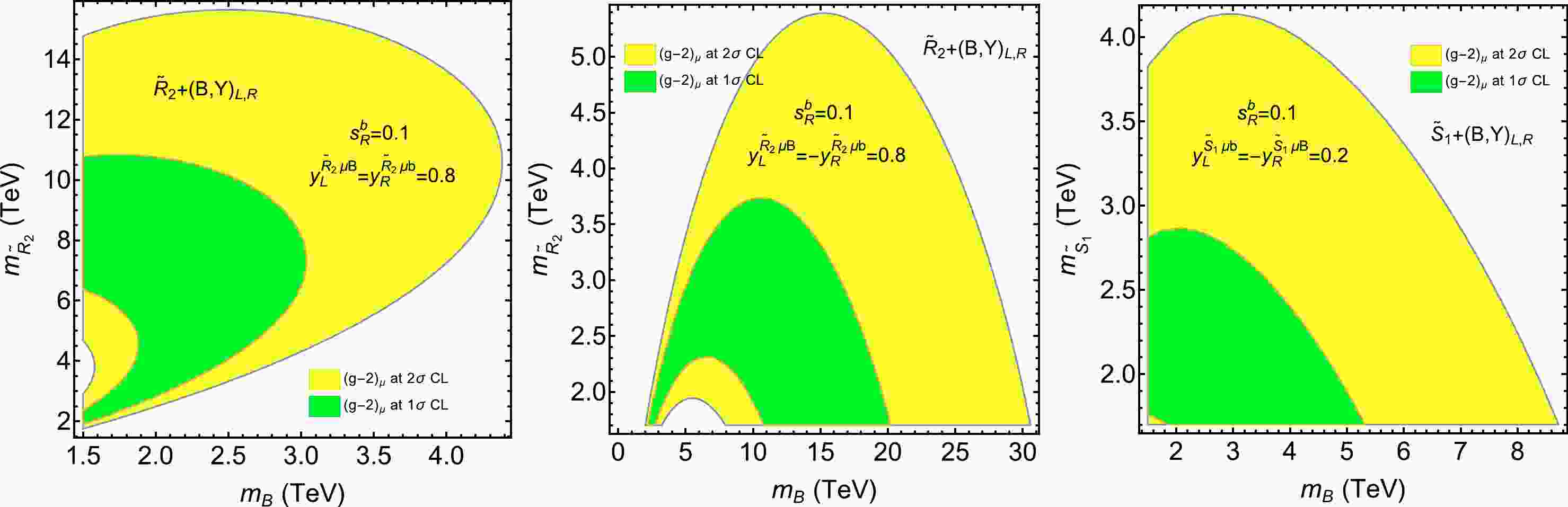
$ s_R^b $ and LQ Yukawa couplings to constrain the$ m_B $ and$ m_{ \mathrm{LQ}} $ . Fig. 1 presents the$ (g-2)_{\mu} $ allowed regions in the plane of$ m_B-m_{ \mathrm{LQ}} $ . As shown,$ m_B<m_{\tilde{R}_2} $ and$ m_B>m_{\tilde{R}_2} $ are favored in the left and middle plots, respectively. This can be understood from the asymptotic behaviours$f_{LR}^{\tilde{R}_2\mu b}(x)\sim -\log(x)/2 > 0$ for$ x\rightarrow0 $ and$f_{LR}^{\tilde{R}_2\mu b}(x) \sim-1/(4x) < 0$ for$ x\rightarrow \infty $ . To produce a positive$ \Delta a_{\mu} $ ,$ m_B<m_{\tilde{R}_2} $ and$ m_B>m_{\tilde{R}_2} $ are favored for$ \mathrm{Re}[y_L^{\tilde{R}_2\mu B}(y_R^{\tilde{R}_2\mu b})^\ast]>0 $ and$ \mathrm{Re}[y_L^{\tilde{R}_2\mu B}(y_R^{\tilde{R}_2\mu b})^\ast]<0 $ , respectively. The$ f_{LR}^{\tilde{S}_1\mu b}(x) $ has asymptotic behaviours$f_{LR}^{\tilde{S}_1\mu b}(x)\sim \log(x)/2 < 0$ for$ x\rightarrow0 $ and$f_{LR}^{\tilde{S}_1\mu b}(x)\sim-5/(4x) < 0$ for$ x\rightarrow \infty $ . To produce a positive$ \Delta a_{\mu} $ ,$ \mathrm{Re}[y_R^{\tilde{S}_1\mu B}(y_L^{\tilde{S}_1\mu b})^\ast]<0 $ is favored. Furthermore, the allowed regions in the plane of$ m_B-m_{ \mathrm{LQ}} $ are sensitive to the choice of$ y_{L,R}^{ \mathrm{LQ}\mu q} $ . Generally, a larger$ |y_{L,R}^{ \mathrm{LQ}\mu q}| $ corresponds to a larger$ m_B $ and$ m_{ \mathrm{LQ}} $ .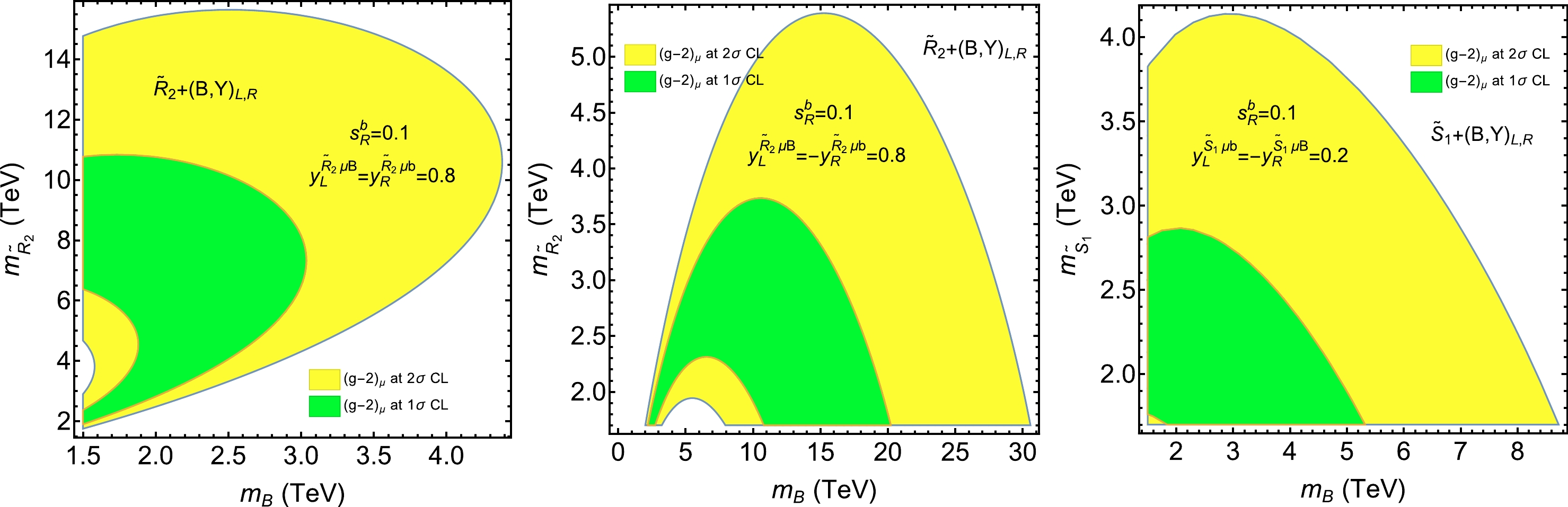
Figure 1. (color online)
$ (g-2)_{\mu} $ allowed regions at$ 1\sigma $ (green) and$ 2\sigma $ (yellow) CLs with$ s_R^b=0.1 $ . The parameters are chosen as$ y_L^{\tilde{R}_2\mu B}=y_R^{\tilde{R}_2\mu b}=0.8 $ in the$ \tilde{R}_2+(B,Y) $ model (left),$ y_L^{\widetilde{R}_2\mu B}=-y_R^{\tilde{R}_2\mu b}=0.8 $ in the$ \tilde{R}_2+(B,Y) $ model (middle), and$ y_L^{\tilde{S}_1\mu b}=-y_R^{\tilde{S}_1\mu B}=0.2 $ in the$ \tilde{S}_1+(B,Y) $ model (right). -
In Table 4, we list the main LQ and VLQ decay channels
2 . The decay formulae of LQ and VLQ are given in Appendices A and B, respectively. For the scenario of$ m_{ \mathrm{LQ}}>m_B $ , there are new LQ decay channels. When searching for the LQ$ \tilde{R}_2^{2/3} $ , we propose the$ \mu j_bZ $ and$ \mu j_bh $ signatures. When searching for the LQ$ \tilde{R}_2^{-1/3} $ , we propose the$ \mu j_bW $ signatures. When searching for the LQ$ \tilde{S}_1 $ , we propose the$ \mu j_bZ $ ,$ \mu j_bh $ ,$ \not {E_T}j_bW $ signatures. For the scenario of$ m_{ \mathrm{LQ}}<m_B $ , there are new VLQ decay channels. When searching for the VLQ B, we propose the$ \mu^+\mu^-j_b $ signatures. When searching for the VLQ Y, we propose the$ \mu\; \not {E_T}j_b $ signatures. It seems that such decay channels have not been searched for by the experimental collaborations.Model Scenario LQ decay VLQ decay new signatures $ \tilde{R}_2+(B,Y)_{L,R} $ 

$ m_{ \mathrm{LQ}}>m_B $ 

$ \tilde{R}_2^{2/3}\rightarrow \mu^+b,\mu^+B $ 

$ B\rightarrow bZ,bh $ 

$ \tilde{R}_2^{2/3}\rightarrow \mu j_bZ,\mu j_bh $ 

$ \tilde{R}_2^{-1/3}\rightarrow \mu^+Y,\nu_Lb $ 

$ Y\rightarrow bW^- $ 

$ \tilde{R}_2^{-1/3}\rightarrow \mu j_bW $ 

$ m_{ \mathrm{LQ}}<m_B $ 

$ \tilde{R}_2^{2/3}\rightarrow \mu^+b $ 

$ B\rightarrow bZ,bh,\mu^-\tilde{R}_2^{2/3} $ 

$ B\rightarrow \mu^+\mu^-j_b $ 

$ \tilde{R}_2^{-1/3}\rightarrow \nu_Lb $ 

$ Y\rightarrow bW^-,\mu^-\tilde{R}_2^{-1/3} $ 

$ Y\rightarrow \mu \not {E_T}j_b $ 

$ \tilde{S}_1+(B,Y)_{L,R} $ 

$ m_{ \mathrm{LQ}}>m_B $ 

$ \tilde{S}_1\rightarrow \mu^+\bar{b},\mu^+\bar{B},\nu_L\bar{Y} $ 

$ B\rightarrow bZ,bh $ 

$ \tilde{S}_1\rightarrow \mu j_bZ $ ,

$ \mu j_bh $ ,

$ \not {E_T}j_bW $ 

$ Y\rightarrow bW^- $ 

$ m_{ \mathrm{LQ}}<m_B $ 

$ \tilde{S}_1\rightarrow \mu^+\bar{b} $ 

$ B\rightarrow bZ,bh,\mu^+(\tilde{S}_1)^{\ast} $ 

$ B\rightarrow \mu^+\mu^-j_b $ 

$ Y\rightarrow bW^-,\nu_L(\tilde{S}_1)^{\ast} $ 

$ Y\rightarrow \mu \not {E_T}j_b $ 

Table 4. In the third column, we show the main LQ decay channels. In the fourth column, we show the main VLQ decay channels. In the fifth column, we show the new LQ or VLQ signatures.
To estimate the effects of new decay channels, we will compare the ratios of new partial decay widths with the traditional ones. Because of gauge symmetry, the different partial decay widths can be correlated. Then, we choose the following four ratios:
$ \begin{aligned}[b]&\frac{\Gamma(\tilde{R}_2^{2/3}\rightarrow \mu^+B)}{\Gamma(\tilde{R}_2^{2/3}\rightarrow \mu^+b)}\sim\frac{|y_L^{\tilde{R}_2\mu B}|^2}{|y_R^{\tilde{R}_2\mu b}|^2},\quad\frac{\Gamma(\tilde{S}_1\rightarrow \mu^+\bar{B})}{\Gamma(\tilde{S}_1\rightarrow \mu^+\bar{b})}\sim\frac{|y_R^{\tilde{S}_1\mu B}|^2}{|y_L^{\tilde{S}_1\mu b}|^2},\\&\frac{\Gamma(B\rightarrow \mu^-\tilde{R}_2^{2/3})}{\Gamma(B\rightarrow bh)}\sim\frac{v^2|y_L^{\tilde{R}_2\mu B}|^2}{m_B^2(s_R^b)^2},\quad\frac{\Gamma(B\rightarrow \mu^+(\tilde{S}_1)^{\ast})}{\Gamma(B\rightarrow bh)}\sim\frac{v^2|y_R^{\tilde{S}_1\mu B}|^2}{m_B^2(s_R^b)^2}. \end{aligned} $

(18) In Fig. 2, we show the contour plots of above four ratios under the consideration of
$ (g-2)_{\mu} $ constraints. In these plots, we include the full contributions. We find that the new LQ decay channels can become important for larger$ |y_L^{\tilde{R}_2\mu B}| $ in the$ \tilde{R}_2+(B,Y)_{L,R} $ model and$ |y_R^{\tilde{S}_1\mu B}| $ in the$ \tilde{S}_1+(B,Y)_{L,R} $ model. As for the VLQ decay, the importance of new decay channels depends significantly on$ s_R^b $ . For$ s_R^b=0.1 $ and$m_B=2.5 ~\mathrm{TeV}$ , the new VLQ decay channels are less significant. For smaller$ s_R^b $ , the new VLQ decay channels can play an important role.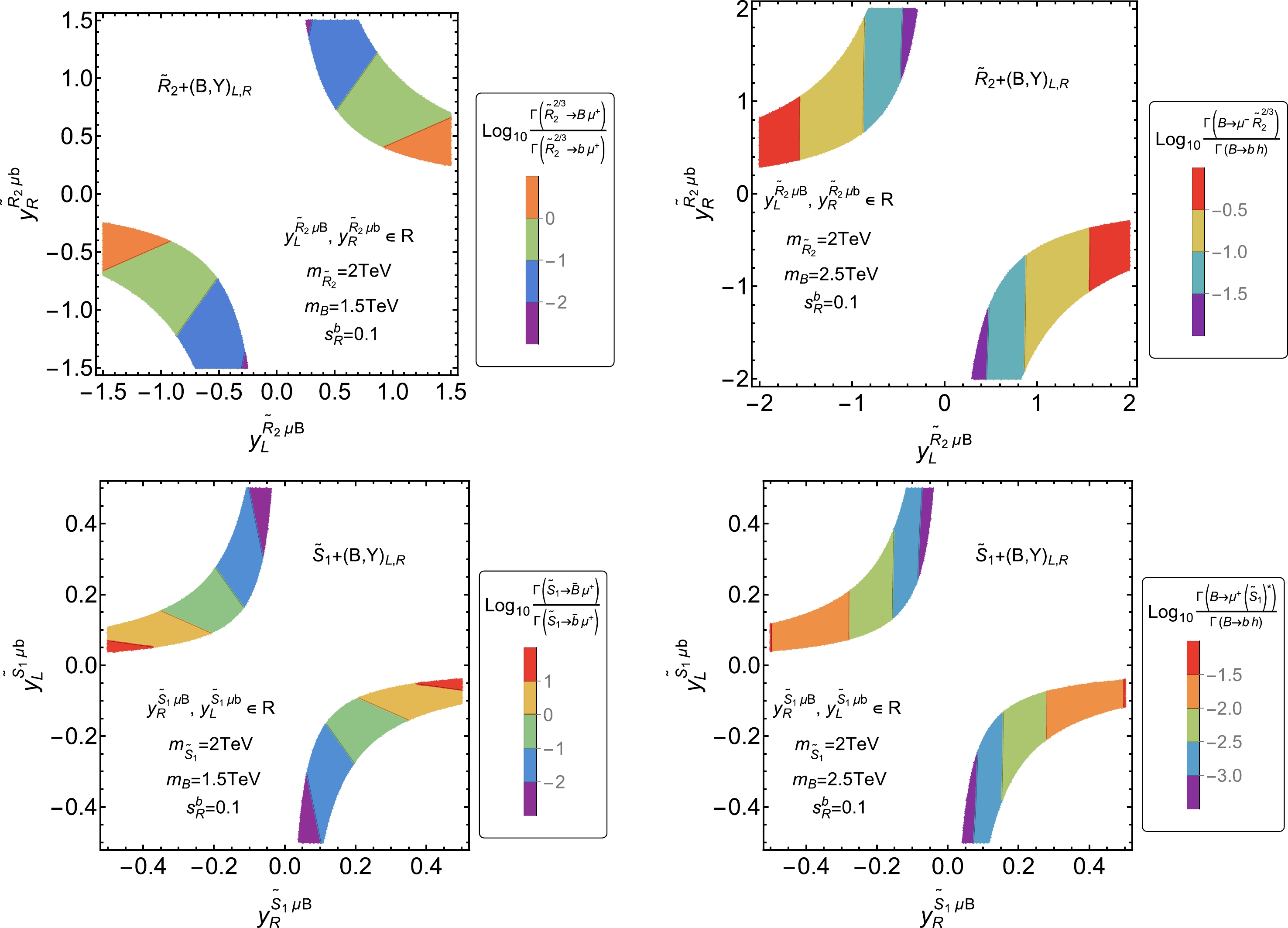
Figure 2. (color online) Contour plots of
$ \log_{10}\frac{\Gamma(\tilde{R}_2^{2/3}\rightarrow \mu^+B)}{\Gamma(\tilde{R}_2^{2/3}\rightarrow \mu^+b)} $ (upper left),$ \log_{10}\frac{\Gamma(\tilde{S}_1\rightarrow \mu^+\bar{B})}{\Gamma(\tilde{S}_1\rightarrow \mu^+\bar{b})} $ (lower left),$ \log_{10}\frac{\Gamma(B\rightarrow \mu^-\tilde{R}_2^{2/3})}{\Gamma(B\rightarrow bh)} $ (upper right), and$ \log_{10}\frac{\Gamma(B\rightarrow \mu^+(\tilde{S}_1)^{\ast})}{\Gamma(B\rightarrow bh)} $ (lower right), where the colored regions are allowed by the$ (g-2)_{\mu} $ at$ 2\sigma $ CL. For the LQ decay, we choose$m_B=1.5 ~\mathrm{TeV}$ and$m_{ \mathrm{LQ}}=2 ~\mathrm{TeV}$ . For the VLQ decay, we choose$m_B=2.5 ~\mathrm{TeV}$ and$m_{ \mathrm{LQ}}=2 ~\mathrm{TeV}$ .For the LQ and VLQ production at hadron colliders, there are pair and single production channels, which are very sensitive to the LQ and VLQ masses. We can adopt the FeynRules [54] to generate the model files and compute the cross sections with MadGraph5
$ {}_{-} $ aMC@NLO [55]. For the 2 TeV scale LQ pair production [56−58], the cross section can be$\sim0.01 ~\mathrm{fb}$ at the 13 TeV LHC. For the 1.5 TeV and 2.5 TeV scale VLQ pair production [59−61], the cross section can be$\sim2~ \mathrm{fb}$ and$\sim0.01~ \mathrm{fb}$ at the 13 TeV LHC. For the single LQ and VLQ production channels, they depend on the electroweak couplings [42, 62, 63]. In the parameter space of large LQ Yukawa couplings, the single LQ production can be important, which may give some constraints at HL-LHC. To generate enough events, higher energy hadron colliders, for example, 27 and 100 TeV, can be necessary. In addition to the collider direct search, there can be indirect footprints, for example, B physics related decay modes$ \Upsilon\rightarrow \mu^+\mu^-,\nu\bar{\nu}\gamma $ . If we consider a more complex flavour structure (e.g., turn on the$ \mathrm{LQ}\mu s $ interaction), this can affect the$ B\rightarrow K\mu^+\mu^- $ channel. Here, we will not study this detailed phenomenology. -
In this study, we investigate the scalar LQ and VLQ extended models to explain the
$ (g-2)_{\mu} $ anomaly. Then, we find two new models$ \tilde{R}_2/\tilde{S}_1+(B,Y)_{L,R} $ , which can lead to the B quark chiral enhancements because of the bottom and bottom partner mixing. In the numerical analysis, we consider two scenarios:$ m_{ \mathrm{LQ}}>m_B $ and$ m_{ \mathrm{LQ}}<m_B $ . After considering the experimental constraints, we choose relative light masses, which are adopted to be$(m_B,m_{ \mathrm{LQ}})=(1.5 ~\mathrm{TeV},2 ~\mathrm{TeV})$ for the first scenario and$(m_B,m_{ \mathrm{LQ}})=(2.5 ~\mathrm{TeV},2~ \mathrm{TeV})$ for the second scenario. In the$ \tilde{R}_2+(B,Y)_{L,R} $ model, the$ | \mathrm{Re}[y_L^{\tilde{R}_2\mu B}(y_R^{\tilde{R}_2\mu b})^\ast]| $ is bounded to be$ \mathcal{O}(1) $ , because$ f_{LR}^{\tilde{R}_2\mu b}(x) $ vanishes accidentally as$ m_B= m_{\tilde{R}_2} $ . Meanwhile, we can expect smaller$ | \mathrm{Re}[y_L^{\tilde{R}_2\mu B}(y_R^{\tilde{R}_2\mu b})^\ast]| $ for largely splitted$ m_{\tilde{R}_2} $ and$ m_B $ . In the$ \tilde{S}_1+(B,Y)_{L,R} $ model, the$ \mathrm{Re}[y_R^{\tilde{S}_1\mu B}(y_L^{\tilde{S}_1\mu b})^\ast] $ is bounded to the range$ (-0.06, -0.02) $ at a$ 2\sigma $ CL if$ s_R^b=0.1 $ .Under the constraints from
$ (g-2)_{\mu} $ , we propose new LQ and VLQ search channels. In the scenario of$ m_{ \mathrm{LQ}}>m_B $ , there are new LQ decay channels:$ \tilde{R}_2^{2/3}\rightarrow \mu^+B $ ,$ \tilde{R}_2^{-1/3}\rightarrow \mu^+Y $ , and$ \tilde{S}_1\rightarrow \mu^+\bar{B},\nu_L\bar{Y} $ . For larger$ y_L^{\tilde{R}_2\mu B} $ and$ y_R^{\tilde{S}_1\mu B} $ , it is important to take into account these decay channels. In the scenario of$ m_{ \mathrm{LQ}}<m_B $ , there are new VLQ decay channels:$ B\rightarrow \mu^-\tilde{R}_2^{2/3},\mu^+(\tilde{S}_1)^{\ast} $ and$Y\rightarrow \mu^-\tilde{R}_2^{-1/3},~ \nu_L(\tilde{S}_1)^{\ast}$ . For$ s_R^b=0.1 $ , these channels are negligible compared with the traditional$B\rightarrow bZ,~bh$ and$ Y\rightarrow bW^- $ channels. For smaller$ s_R^b $ , these new VLQ decay channels can also become important.Note added: In a prevoius study [64], the authors examined the model with
$ \tilde{R}_2 $ ,$ S_3 $ , and$ (B,Y)_{L,R} $ . In this work, they did not consider the bottom and B quark mixing, and the chiral enhancements were produced through the$ \tilde{R}_2 $ and$ S_3 $ mixing. In [65], the authors explained the$ (g-2)_{\mu} $ and B physics anomalies in the$ S_1+(B,Y)_{L,R} $ model. -
When the
$ \tilde{R}_2 $ masses are degenerate, there are no gauge boson decay channels such as$ \tilde{R}_2^{2/3}\rightarrow \tilde{R}_2^{-1/3}W^+ $ . For the$ \tilde{R}_2^{2/3} $ to$ \mu^+b $ and$ \mu^+B $ decay channels, the widths are calculated as$ \begin{aligned}[b]\\[-5pt]\Gamma(\tilde{R}_2^{2/3}\rightarrow \mu^+b)=&\frac{m_{\tilde{R}_2}}{16\pi}\sqrt{\left(1-\frac{m_{\mu}^2+m_b^2}{m_{\tilde{R}_2}^2}\right)^2-\frac{4m_{\mu}^2m_b^2}{m_{\tilde{R}_2}^4}}\;\\& \times\Bigg\{\Bigg(1-\frac{m_{\mu}^2+m_b^2}{m_{\tilde{R}_2}^2}\Bigg)[|y_L^{\tilde{R}_2\mu B}|^2(s_L^b)^2+|y_R^{\tilde{R}_2\mu b}|^2(c_R^b)^2]+\frac{4m_{\mu}m_b}{m_{\tilde{R}_2}^2}s_L^bc_R^b \mathrm{Re}[y_L^{\tilde{R}_2\mu B}(y_R^{\tilde{R}_2\mu b})^\ast]\Bigg\},\\\Gamma(\tilde{R}_2^{2/3}\rightarrow \mu^+B)=&\frac{m_{\tilde{R}_2}}{16\pi}\sqrt{\Bigg(1-\frac{m_{\mu}^2+m_B^2}{m_{\tilde{R}_2}^2}\Bigg)^2-\frac{4m_{\mu}^2m_B^2}{m_{\tilde{R}_2}^4}}\; \\&\times\Bigg\{\Bigg(1-\frac{m_{\mu}^2+m_B^2}{m_{\tilde{R}_2}^2}\Bigg)[|y_L^{\tilde{R}_2\mu B}|^2(c_L^b)^2+|y_R^{\tilde{R}_2\mu b}|^2(s_R^b)^2]-\frac{4m_{\mu}m_B}{m_{\tilde{R}_2}^2}c_L^bs_R^b \mathrm{Re}[y_L^{\tilde{R}_2\mu B}(y_R^{\tilde{R}_2\mu b})^\ast]\Bigg\}. \end{aligned}\tag{A1} $ 
For the
$ \tilde{R}_2^{-1/3} $ to$ \mu^+Y,\nu_Lb,\nu_LB $ decay channels, the widths are calculated as$ \begin{aligned}[b]\Gamma(\tilde{R}_2^{-1/3}\rightarrow \mu^+Y)=\frac{m_{\tilde{R}_2}}{16\pi}\sqrt{\left(1-\frac{m_{\mu}^2+m_Y^2}{m_{\tilde{R}_2}^2}\right)^2-\frac{4m_{\mu}^2m_Y^2}{m_{\tilde{R}_2}^4}}\left(1-\frac{m_{\mu}^2+m_Y^2}{m_{\tilde{R}_2}^2}\right)|y_L^{\tilde{R}_2\mu B}|^2, \end{aligned} $

$ \begin{aligned}[b]&\Gamma(\tilde{R}_2^{-1/3}\rightarrow \nu_Lb)=\frac{m_{\tilde{R}_2}}{16\pi}\left(1-\frac{m_b^2}{m_{\tilde{R}_2}^2}\right)^2|y_R^{\tilde{R}_2\mu b}|^2(c_R^b)^2,\\&\Gamma(\tilde{R}_2^{-1/3}\rightarrow \nu_LB)=\frac{m_{\tilde{R}_2}}{16\pi}\left(1-\frac{m_B^2}{m_{\tilde{R}_2}^2}\right)^2|y_R^{\tilde{R}_2\mu b}|^2(s_R^b)^2. \end{aligned}\tag{A2} $

Considering
$ m_{\mu},m_b\ll m_B $ and$ \theta_{L,R}^b\ll1 $ , we have the following approximations:$ \begin{aligned}[b]&\Gamma(\tilde{R}_2^{2/3}\rightarrow \mu^+B)\approx\Gamma(\tilde{R}_2^{-1/3}\rightarrow \mu^+Y)\approx\frac{m_{\tilde{R}_2}}{16\pi}\Bigg(1-\frac{m_B^2}{m_{\tilde{R}_2}^2}\Bigg)^2|y_L^{\tilde{R}_2\mu B}|^2,\\&\Gamma(\tilde{R}_2^{2/3}\rightarrow \mu^+b)\approx\Gamma(\tilde{R}_2^{-1/3}\rightarrow \nu_Lb)\approx\frac{m_{\tilde{R}_2}}{16\pi}|y_R^{\tilde{R}_2\mu b}|^2. \end{aligned}\tag{A3} $

For the
$ \tilde{S}_1 $ to$ \mu^+\bar{b},\mu^+\bar{B},\nu_L\bar{Y} $ decay channels, the widths are calculated as$ \begin{aligned}[b]\Gamma(\tilde{S}_1\rightarrow \mu^+\bar{b})=&\frac{m_{\tilde{S}_1}}{16\pi}\sqrt{\Bigg(1-\frac{m_{\mu}^2+m_b^2}{m_{\tilde{S}_1}^2}\Bigg)^2-\frac{4m_{\mu}^2m_b^2}{m_{\tilde{S}_1}^4}}\; \\&\times\Bigg\{\Bigg(1-\frac{m_{\mu}^2+m_b^2}{m_{\tilde{S}_1}^2}\Bigg)[|y_R^{\tilde{S}_1\mu B}|^2(s_L^b)^2+|y_L^{\tilde{S}_1\mu b}|^2(c_R^b)^2]+\frac{4m_{\mu}m_b}{m_{\tilde{S}_1}^2}s_L^bc_R^b \mathrm{Re}[y_R^{\tilde{S}_1\mu B}(y_L^{\tilde{S}_1\mu b})^\ast]\Bigg\},\\\Gamma(\tilde{S}_1\rightarrow \mu^+\bar{B})=&\frac{m_{\tilde{S}_1}}{16\pi}\sqrt{\Bigg(1-\frac{m_{\mu}^2+m_B^2}{m_{\tilde{S}_1}^2}\Bigg)^2-\frac{4m_{\mu}^2m_B^2}{m_{\tilde{S}_1}^4}}\; \\&\times\Big\{(1-\frac{m_{\mu}^2+m_B^2}{m_{\tilde{S}_1}^2})[|y_R^{\tilde{S}_1\mu B}|^2(c_L^b)^2+|y_L^{\tilde{S}_1\mu b}|^2(s_R^b)^2]-\frac{4m_{\mu}m_B}{m_{\tilde{S}_1}^2}c_L^bs_R^b \mathrm{Re}[y_R^{\tilde{S}_1\mu B}(y_L^{\tilde{S}_1\mu b})^\ast]\Bigg\},\\\Gamma(\tilde{S}_1\rightarrow \nu_L\bar{Y})=&\frac{m_{\tilde{S}_1}}{16\pi}\Bigg(1-\frac{m_Y^2}{m_{\tilde{S}_1}^2}\Bigg)^2|y_R^{\tilde{S}_1\mu B}|^2. \end{aligned}\tag{A4} $

Considering
$ m_{\mu},m_b\ll m_B $ and$ \theta_{L,R}^b\ll1 $ , we have the following approximations:$ \begin{aligned}[b]&\Gamma(\tilde{S}_1\rightarrow \mu^+\bar{B})\approx\Gamma(\tilde{S}_1\rightarrow \nu_L\bar{Y})\approx\frac{m_{\tilde{S}_1}}{16\pi}\Bigg(1-\frac{m_B^2}{m_{\tilde{S}_1}^2}\Bigg)^2|y_R^{\tilde{S}_1\mu B}|^2,\\&\Gamma(\tilde{S}_1\rightarrow \mu^+\bar{b})\approx\frac{m_{\tilde{S}_1}}{16\pi}|y_L^{\tilde{S}_1\mu b}|^2. \end{aligned} \tag{A5}$

-
If
$ m_B\sim \mathrm{TeV} $ and$ \theta_R^b\ll0.1 $ , we have$m_B-m_Y\approx m_B(s_R^b)^2/2\lesssim5 ~\mathrm{GeV}$ , which leads to the kinematic prohibition of some decay channels. For the$ Y\rightarrow bW^- $ decay channel, the width is calculated as$ \Gamma(Y\rightarrow bW^-)=\frac{g^2}{64\pi m_Y}\sqrt{\Bigg(1-\frac{m_b^2+m_W^2}{m_Y^2}\Bigg)^2-\frac{4m_b^2m_W^2}{m_Y^4}}\cdot\Bigg\{[(s_L^b)^2+(s_R^b)^2]\frac{(m_Y^2-m_b^2)^2+m_W^2(m_Y^2+m_b^2)-2m_W^4}{m_W^2}-12m_Ym_bs_L^bs_R^b\Bigg\}. \tag{B1} $

For the
$ B\rightarrow bZ,~bh,~tW^- $ decay channels, the widths are calculated as$ \begin{aligned}[b]\Gamma(B\rightarrow bh)=&\frac{m_B}{32\pi}\sqrt{\Bigg(1-\frac{m_b^2+m_h^2}{m_B^2}\Bigg)^2-\frac{4m_b^2m_h^2}{m_B^4}}\Bigg[\Bigg(1+\frac{m_b^2-m_h^2}{m_B^2}\Bigg)\frac{m_b^2+m_B^2}{v^2}+4\frac{m_b^2}{v^2}\Bigg](s_R^b)^2(c_R^b)^2, \\\Gamma(B\rightarrow bZ)=&\frac{g^2}{32\pi c_W^2m_B}\sqrt{\Bigg(1-\frac{m_b^2+m_Z^2}{m_B^2}\Bigg)^2-\frac{4m_b^2m_Z^2}{m_B^4}}\\&\times\Bigg\{\Bigg[(s_L^bc_L^b)^2+\frac{(s_R^bc_R^b)^2}{4}\Bigg]\frac{(m_B^2-m_b^2)^2+m_Z^2(m_B^2+m_b^2)-2m_Z^4}{m_Z^2}-6m_Bm_bs_L^bs_R^bc_L^bc_R^b\Bigg\},\\\Gamma(B\rightarrow tW^-)=&\frac{g^2(s_L^b)^2}{64\pi}\sqrt{\Bigg(1-\frac{m_t^2+m_W^2}{m_B^2}\Bigg)^2-\frac{4m_t^2m_W^2}{m_B^4}}\frac{(m_B^2-m_t^2)^2+m_W^2(m_B^2+m_t^2)-2m_W^4}{m_W^2m_B}. \end{aligned}\tag{B2} $

Considering
$m_b,~m_t,~m_Z,~m_W\ll m_B$ and$ \theta_{L,R}^b\ll1 $ , we have the following approximations:$ \begin{aligned}[b]&\Gamma(B\rightarrow bZ)\approx\Gamma(B\rightarrow bh)\approx\frac{1}{2}\Gamma(Y\rightarrow bW^-)\approx\frac{m_B^3}{32\pi v^2}(s_R^b)^2,\\&\Gamma(B\rightarrow tW^-)\approx\frac{m_b^2m_B}{16\pi v^2}(s_R^b)^2. \end{aligned}\tag{B3} $

In the
$ \tilde{R}_2+(B,Y)_{L,R} $ model, the VLQ can also decay into the$ \tilde{R}_2 $ final state. For the$ Y\rightarrow \mu^-\tilde{R}_2^{-1/3} $ decay channel, the width is calculated as$ \Gamma(Y\rightarrow \mu^-\tilde{R}_2^{-1/3})=\frac{m_Y}{32\pi}\sqrt{\Bigg(1-\frac{m_{\mu}^2+m_{\tilde{R}_2}^2}{m_Y^2}\Bigg)^2-\frac{4m_{\mu}^2m_{\tilde{R}_2}^2}{m_Y^4}}\Bigg(1+\frac{m_{\mu}^2-m_{\tilde{R}_2}^2}{m_Y^2}\Bigg)|y_L^{\tilde{R}_2\mu B}|^2. \tag{B4} $

For the
$ B\rightarrow \mu^-\tilde{R}_2^{2/3},~\nu_L\tilde{R}_2^{-1/3} $ decay channels, the widths are calculated as$ \begin{aligned}[b]\Gamma(B\rightarrow \mu^-\tilde{R}_2^{2/3})=&\frac{m_B}{32\pi}\sqrt{\Bigg(1-\frac{m_{\mu}^2+m_{\tilde{R}_2}^2}{m_B^2}\Bigg)^2-\frac{4m_{\mu}^2m_{\tilde{R}_2}^2}{m_B^4}}\; \\&\times\Bigg\{\Bigg(1+\frac{m_{\mu}^2-m_{\tilde{R}_2}^2}{m_B^2}\Bigg)[|y_L^{\tilde{R}_2\mu B}|^2(c_L^b)^2+|y_R^{\tilde{R}_2\mu b}|^2(s_R^b)^2]+\frac{4m_{\mu}m_{\tilde{R}_2}}{m_B^2}c_L^bs_R^b \mathrm{Re}[y_L^{\tilde{R}_2\mu B}(y_R^{\tilde{R}_2\mu b})^\ast]\Big\},\\\Gamma(B\rightarrow \nu_L\tilde{R}_2^{-1/3})=&\frac{m_B}{32\pi}\Bigg(1-\frac{m_{\tilde{R}_2}^2}{m_B^2}\Bigg)^2|y_R^{\tilde{R}_2\mu b}|^2(s_R^b)^2. \end{aligned}\tag{B5} $

Considering
$ m_{\mu}\ll m_B $ and$ \theta_{L,R}^b\ll1 $ , we have the following approximations:$\Gamma(B\rightarrow \mu^-\tilde{R}_2^{2/3})\approx\Gamma(Y\rightarrow \mu^-\tilde{R}_2^{-1/3})\approx\frac{m_B}{32\pi}\Bigg(1-\frac{m_{\tilde{R}_2}^2}{m_B^2}\Bigg)^2|y_L^{\tilde{R}_2\mu B}|^2. \tag{B6} $

In the
$ \tilde{S}_1+(B,Y)_{L,R} $ model, the VLQ can also decay into the$ \tilde{S}_1 $ final state. For the$ Y\rightarrow \nu_L(\tilde{S}_1)^{\ast} $ decay channel, the width is calculated as$\Gamma(Y\rightarrow \nu_L(\tilde{S}_1)^{\ast})=\frac{m_Y}{32\pi}\Bigg(1-\frac{m_{\tilde{S}_1}^2}{m_Y^2}\Bigg)^2|y_R^{\tilde{S}_1\mu B}|^2. \tag{B7}$

For the
$ B\rightarrow \mu^+(\tilde{S}_1)^{\ast} $ decay channel, the width is calculated as$ \begin{aligned}[b]\Gamma(B\rightarrow \mu^+(\tilde{S}_1)^{\ast})=&\frac{m_B}{32\pi}\sqrt{\Bigg(1-\frac{m_{\mu}^2+m_{\tilde{S}_1}^2}{m_B^2}\Bigg)^2-\frac{4m_{\mu}^2m_{\tilde{S}_1}^2}{m_B^4}}\;\\&\times\Bigg\{\Bigg(1+\frac{m_{\mu}^2-m_{\tilde{S}_1}^2}{m_B^2}\Bigg)[|y_R^{\tilde{S}_1\mu B}|^2(c_L^b)^2+|y_L^{\tilde{S}_1\mu b}|^2(s_R^b)^2]+\frac{4m_{\mu}}{m_B}c_L^bs_R^b \mathrm{Re}[y_R^{\tilde{S}_1\mu B}(y_L^{\tilde{S}_1\mu b})^\ast]\Bigg\}. \end{aligned}\tag{B8} $

Considering
$ m_{\mu}\ll m_B $ and$ \theta_{L,R}^b\ll1 $ , we have the following approximations:$ \Gamma(B\rightarrow \mu^+(\tilde{S}_1)^{\ast})\approx\Gamma(Y\rightarrow \nu_L(\tilde{S}_1)^{\ast})\approx\frac{m_B}{32\pi}\Bigg(1-\frac{m_{\tilde{S}_1}^2}{m_B^2}\Bigg)^2|y_R^{\tilde{S}_1\mu B}|^2. \tag{B9} $

Scalar leptoquark and vector-like quark extended models as the explanation of the muon g–2 anomaly: bottom partner chiral enhancement case
- Received Date: 2023-02-14
- Available Online: 2023-07-15
Abstract: Leptoquark (LQ) models are well motivated solutions to the


 DownLoad: