Loading [MathJax]/jax/element/mml/optable/MathOperators.js

Neutron skin thickness of 90Zr and symmetry energy constrained by charge exchange spin-dipole excitations

  • The charge exchange spin-dipole (SD) excitations of 90Zr are studied using the Skyrme Hartee-Fock plus proton-neutron random phase approximation with SAMi-J interactions. The experimental value of the model-independent sum rule obtained from the SD strength distributions of 90Zr(p, n)90Nb and 90Zr(n, p)90Y is used to deduce the neutron skin thickness. The neutron skin thickness Δrnp of 90Zr is extracted as 0.083±0.032 fm, which is similar to the results of other studies. Based on the correlation analysis of the neutron skin thickness Δrnp and the nuclear symmetry energy J as well as its slope parameter L, a constraint from the extracted Δrnp leads to the limitation of J to 29.2±2.6 MeV and L to 53.3±28.2 MeV.
      PCAS:
    • 21.65.Mn(Equations of state of nuclear matter)
  • The (g2)μ anomaly is a longstanding puzzle in the standard model (SM) of elementary particle physics. It was first announced by the BNL E821 experiment [1]. Last year, the FNAL muon g2 experiment revealed increased deviation from the SM prediction [2]. When combining the BNL and FNAL data, the averaged result is aExpμ=116592061(41)×1011. Compared to the SM prediction aSMμ=116591810(43)×1011 [323], the deviation is ΔaμaExpμaSMμ=(251±59)×1011, which shows a 4.2σ discrepancy. Many new physics models were proposed to explain the anomaly [2429].

    For the mediators with mass above the TeV level, the chiral enhancements are required, which can appear when left-handed and right-handed muons couple to a heavy fermion simultaneously. In the new lepton extended models [3033], the chiral enhancements originate from the large lepton mass. The LQ models are an alternative choice [3440], in which the chiral enhancements originate from the large quark mass. For the minimal LQ models, there are scalar LQs R2/S1 with top quark chiral enhancement and vector LQs V2/U1 with bottom quark chiral enhancement. The LQ can connect the lepton sector and quark sector. On the other hand, the VLQ naturally occurs in many new physics models and is free of quantum anomaly. It can mix with SM quarks and provide new source of CP violation. Hence, the LQ and VLQ extended models can lead to interesting flavour physics in both the lepton sector and quark sector. In our previous study [41], we investigated the scalar LQ and VLQ 1 extended models with top and top partner chiral enhancements. In this study, we investigate the scalar LQ and VLQ extended models, which can produce the bottom partner chiral enhancements. This paper is complementary to our previous paper [41]. Moreover, the top partner and bottom partner lead to different collider signatures.

    In Sec. II, we introduce the models and show the related interactions. Then, we derive the new physics contributions to (g2)μ and perform the numerical analysis in Sec. III. In Sec. IV, we discuss the possible collider phenomenology. Finally, we present a summary and conclusions in Sec. V.

    Typically, there are six types of scalar LQs [35], which carry a conserved quantum number F3B+L. Here, B and L are the baryon and lepton numbers. As for the VLQs, there are seven typical representations [42]. In Table 1, we list their representations and labels.

    Table 1

    Table 1.  Scalar LQ (left) and VLQ (right) representations.
    SU(3)C×SU(2)L×U(1)Y representationlabelFSU(3)C×SU(2)L×U(1)Y representationlabel
    (ˉ3,3,1/3)S32(3,1,2/3)TL,R
    (3,2,7/6)R20(3,1,1/3)BL,R
    (3,2,1/6)˜R20(3,2,7/6)(X,T)L,R
    (ˉ3,1,4/3)˜S12(3,2,1/6)(T,B)L,R
    (3,2,5/6)(B,Y)L,R
    (ˉ3,1,1/3)S12(3,3,2/3)(X,T,B)L,R
    (ˉ3,1,2/3)ˉS12(3,3,1/3)(T,B,Y)L,R
    DownLoad: CSV
    Show Table

    For the six types of scalar LQs and seven types of VLQs, there can be a total of 42 combinations, which are named "LQ+VLQ" for convenience. Only 17 of them can lead to the chiral enhancements. In Table 2, we list these models that feature the chiral enhancements. The contributons in the four models R2+BL,R/(B,Y)L,R and S1+BL,R/(B,Y)L,R are almost the same as those in the minimal R2 and S1 models. There are nine models R2+TL,R/(X,T)L,R/(T,B)L,R/(T,B,Y)L,R and S1+TL,R/(X,T)L,R/(T,B)L,R/(X,T,B)L,R/(T,B,Y)L,R, which produce the top and top partner chiral enhancements. For the two models R2/S3+(X,T,B)L,R, there are top, top partner, bottom, and bottom partner chiral enhancements at the same time. The models including T quarks were investigated in our previous work [41]. Here, we will study the pure bottom partner chirally enhanced models ˜R2/˜S1+(B,Y)L,R.

    Table 2

    Table 2.  Chiral enhancements in the minimal LQ and LQ+VLQ models.
    ModelChiral enhancement
    R2mt/mμ
    S1mt/mμ
    R2+BL,R/(B,Y)L,Rmt/mμ
    S1+BL,R/(B,Y)L,Rmt/mμ
    R2+TL,R/(X,T)L,R/(T,B)L,R/(T,B,Y)L,Rmt/mμ,mT/mμ
    S1+TL,R/(X,T)L,R/(T,B)L,R/(X,T,B)L,R/(T,B,Y)L,Rmt/mμ,mT/mμ
    R2+(X,T,B)L,Rmt/mμ,mT/mμ,mb/mμ,mB/mμ
    S3+(X,T,B)L,Rmt/mμ,mT/mμ,mb/mμ,mB/mμ
    ˜R2+(B,Y)L,Rmb/mμ,mB/mμ
    ˜S1+(B,Y)L,Rmb/mμ,mB/mμ
    DownLoad: CSV
    Show Table

    Let us start with the (B,Y)L,R related Higgs Yukawa interactions. In the gauge eigenstates, there are two interactions ¯QLidjRϕ and (¯BL,¯YL)djR˜ϕ and the mass term MB(ˉBB+ˉYY). Here, we define the SM Higgs doublet ˜ϕiσ2ϕ with σa(a=1,2,3) to be the Pauli matrices. The QiL and diR (i=1,2,3) represent the SM quark fields. We can parametrize ϕ as [0,(v+h)/2]T in the unitary gauge. After the electroweak symmetry breaking (EWSB), there are mixings between di and B. For simplicity, we only consider mixing between the third generation and B quark. Thus, we can perform the following transformations to rotate b and B quarks into mass eigenstates:

    [bLBL][cbLsbLsbLcbL][bLBL],[bRBR][cbRsbRsbRcbR][bRBR].

    (1)

    Here, sbL,R and cbL,R are abbreviations of sinθbL,R and cosθbL,R, respectively. In fact, θbL can be correlated with θbR through the relation tanθbL=mbtanθbR/mB [42]. Here, mb and mB represent the physical b and B quark masses, respectively. Additionally, the mass of the Y quark is mY=MB= m2B(cbR)2+m2b(sbR)2. Then, we can choose mB and θbR as the new input parameters. After the transformations in Eq. (1), we obtain the following mass eigenstate Higgs Yukawa interactions:

    LYukawaHmbv(cbR)2hˉbbmBv(sbR)2hˉBBmbvsbRcbRh(ˉbLBR+ˉBRbL)mBvsbRcbRh(ˉBLbR+ˉbRBL).

    (2)

    Note that the Y quark does not interact with Higgs at the tree level.

    Now, let us label the SU(2)L and UY(1) gauge fields as Waμ and Bμ. Then, the electroweak covariant derivative Dμ is defined as μigWaμσa/2igYqBμ for a doublet and μigYqBμ for a singlet, in which Yq is the UY(1) charge of the quark field acted by Dμ. Thus, the related gauge interactions can be written as ¯QLiiDμγμQiL+¯dRiiDμγμdiR+(¯B,¯Y)iDμγμ(B,Y)T. After the EWSB, the W gauge interactions can be written as

    Lg2W+μ(¯tLγμbL+ˉBγμY)+h.c..

    (3)

    The Z gauge interactions can be written as

    LgcW[(12+13s2W)¯bLγμbL+13s2W¯bRγμbR+(12+13s2W)ˉBγμB+(12+43s2W)ˉYγμY]Zμ.

    (4)

    After the rotations in Eq. (1), we have the mass eigenstate W gauge interactions:

    LgaugeBYg2W+μ[cbL¯tLγμbL+sbL¯tLγμBL+cbL¯BLγμYLsbL¯bLγμYL+cbR¯BRγμYRsbR¯bRγμYR]+h.c..

    (5)

    We also have the mass eigenstate Z gauge interactions:

    LgaugeBYgcWZμ[(cbL)2(sbL)22(¯BLγμBL¯bLγμbL)sbLcbL(¯bLγμBL+¯BLγμbL)+(sbR)22¯bRγμbR+(cbR)22¯BRγμBRsbRcbR2(¯bRγμBR+¯BRγμbR)+s2W3(ˉbγμb+ˉBγμB)+(12+4s2W3)ˉYγμY].

    (6)

    Let us denote the SM lepton fields as LiL and eiR. The ˜R2 can be parametrized as [˜R2/32,˜R1/32]T, where the superscript labels the electric charge. Then, the ˜R2 and ˜S1 can induce the following F=0 and F=2 type gauge eigenstate LQ Yukawa interactions:

    L˜R2+(B,Y)L,Rxi¯eiR(˜R2)(BLYL)+yij¯LiLϵ(˜R2)djR+h.c.,

    (7)

    and

    L˜S1+(B,Y)L,Rxij¯eiR(djR)C(˜S1)+yi¯LiLϵ(BLYL)C(˜S1)+h.c..

    (8)

    After the EWSB, they can be parametrized as

    L˜R2+(B,Y)L,Ry˜R2μBLˉμωB(˜R2/32)+y˜R2μbRˉμω+b(˜R2/32)+y˜R2μBLˉμωY(˜R1/32)y˜R2μbR¯νLω+b(˜R1/32)+h.c.,

    (9)

    and

    L˜S1+(B,Y)L,Ry˜S1μbLˉμωbC(˜S1)+y˜S1μBRˉμω+BC(˜S1)y˜S1μBR¯νLω+YC(˜S1)+h.c..

    (10)

    In the above, we define the chiral operators ω± as (1±γ5)/2. After the rotations in Eq. (1), we have the mass eigenstate interactions:

    L˜R2+(B,Y)L,Rˉμ(y˜R2μBLsbLω+y˜R2μbRcbRω+)b(˜R2/32)+ˉμ(y˜R2μBLcbLω+y˜R2μbRsbRω+)B(˜R2/32)+y˜R2μBLˉμωY(˜R1/32)y˜R2μbR¯νLω+(cbRb+sbRB)(˜R1/32)+h.c.,

    (11)

    and

    L˜S1+(B,Y)L,Rˉμ(y˜S1μbLcbRωy˜S1μBRsbLω+)bC(˜S1)+ˉμ(y˜S1μbLsbRω+y˜S1μBRcbLω+)BC(˜S1)y˜S1μBR¯νLω+YC(˜S1)+h.c..

    (12)

    For the LQμq interaction, there are quark-photon and LQ-photon vertex mediated contributions to (g2)μ, which can be described by the functions fq(x) and fS(x). Then, we use the functions fq,SLL(x) and fq,SLR(x) to label the parts without and with chiral enhancements. Starting from the fq,SLL(x) and fq,SLR(x) given in our previous paper [41], let us define the following integrals:

    f˜R2μYLL(x)4fqLL(x)fSLL(x)=3+2x7x2+2x3+2x(4x)logx4(1x)4,f˜R2μbLL(x)fqLL(x)+2fSLL(x)=x[54xx2+(2+4x)logx]4(1x)4,f˜R2μbLR(x)fqLR(x)+2fSLR(x)=54xx2+(2+4x)logx4(1x)3,f˜S1μbLL(x)fqLL(x)+4fSLL(x)=27x+2x2+3x3+2x(14x)logx4(1x)4,f˜S1μbLR(x)fqLR(x)+4fSLR(x)=1+4x5x2(28x)logx4(1x)3.

    (13)

    For the ˜R2+(B,Y)L,R model, there are b, B, and Y quark contributions to the (g2)μ. The complete expression is calculated as

    Δa˜R2+BYμ=m2μ8π2{|y˜R2μBL|2m2˜R1/32f˜R2μYLL(m2Ym2˜R1/32)+|y˜R2μBL|2(sbL)2+|y˜R2μbR|2(cbR)2m2˜R2/32f˜R2μbLL(m2bm2˜R2/32)2mbmμsbLcbRm2˜R2/32Re[y˜R2μBL(y˜R2μbR)]f˜R2μbLR(m2bm2˜R2/32)+|y˜R2μBL|2(cbL)2+|y˜R2μbR|2(sbR)2m2˜R2/32f˜R2μbLL(m2Bm2˜R2/32)+2mBmμcbLsbRm2˜R2/32Re[y˜R2μBL(y˜R2μbR)]f˜R2μbLR(m2Bm2˜R2/32)}.

    (14)

    At the tree level, we have m˜R2/32=m˜R1/32m˜R2. Compared with the bottom partner chirally enhanced contribution (i.e., the f˜R2μbLR(m2Bm2˜R2/32) related term), the non-chirally enhanced parts are suppressed by the factor mμ/(mBsbR)1/(104sbR) and the bottom quark chirally enhanced part is suppressed by the factor (mbsbL)/(mBsbR)(m2b/m2B). For the interesting values of sbR at O(0.010.1), Δa˜R2+BYμ is dominated by the bottom partner chirally enhanced contribution. Then, the above expression can be approximated as

    Δa˜R2+BYμmμmB4π2m2˜R2sbRRe[y˜R2μBL(y˜R2μbR)]f˜R2μbLR(m2Bm2˜R2).

    (15)

    For the ˜S1+(B,Y)L,R model, there are b and B quark contributions to (g2)μ. The complete expression is calculated as

    Δa˜S1+BYμ=m2μ8π2{|y˜S1μBR|2(sbL)2+|y˜S1μbL|2(cbR)2m2˜S1f˜S1μbLL(m2bm2˜S1)2mbmμsbLcbRm2˜S1Re[y˜S1μBR(y˜S1μbL)]f˜S1μbLR(m2bm2˜S1)+|y˜S1μBR|2(cbL)2+|y˜S1μbL|2(sbR)2m2˜S1f˜S1μbLL(m2Bm2˜S1)+2mBmμcbLsbRm2˜S1Re[y˜S1μBR(y˜S1μbL)]f˜S1μbLR(m2Bm2˜S1)}.

    (16)

    Similarly, it can be approximated as

    Δa˜S1+BYμmμmB4π2m2˜S1sbRRe[y˜S1μBR(y˜S1μbL)]f˜S1μbLR(m2Bm2˜S1).

    (17)

    The input parameters are chosen as mμ=105.66 MeV, mb=4.2 GeV, mt=172.5 GeV, GF=1.1664×10⁵ GeV2, mW=80.377 GeV, mZ=91.1876 GeV, and mh=125.25GeV [43]. The v,g,θW are defined by GF=1/(2v2),g=2mW/v, cosθWcW=mW/mZ. There are also new parameters mB, mLQ, θbR, and the LQ Yukawa couplings yLQμqL,R. The VLQ mass can be constrained from the direct search, which is required to be above 1.5 TeV [4447]. The mixing angle is mainly bounded by the electro-weak precision observables (EWPOs). The VLQ contributions to T parameter are suppressed by the factor (sbR)4 or m2b(sbR)2/m2B [48, 49], which leads to a less constrained θbR. The weak isospin third component of BR is positive; thus, the mixing with the bottom quark enhances the right-handed Zbb coupling. As a result, the AbFB deviation [50, 51] can be compensated, which leads to looser constraints on θbR. Conservatively, we can choose the mixing angle sbR to be smaller than 0.1 [42]. The LQ mass can also be constrained from the direct search, which is required to be above 1.7 TeV assuming Br(LQbμ)=1 [52, 53].

    We can choose benchmark points of mB,mLQ,sbR to constrain the LQ Yukawa couplings. Here, we consider two scenarios: mLQ>mB and mLQ<mB. For the scenario of mLQ>mB, we adopt mass parameters of mB= 1.5 TeV and mLQ=2 TeV. For the scenario of mLQ<mB, we adopt mass parameters of mB= 2.5 TeV and mLQ=2 TeV. In Table 3, we give the approximate numerical expressions of Δaμ in the ˜R2/˜S1+(B,Y)L,R models. We also show the allowed ranges for sbR=0.1 and sbR=0.05. Of course, these behaviours can be understood from Eqs. (15) and (17). In the ˜R2+(B,Y)L,R model, f˜R2μbLR(x) vanishes when mB=m˜R2, which causes the |Re[y˜R2μBL(y˜R2μbR)]| to be under the stress of perturbative unitarity. If there is a large hierarchy between mB and m˜R2, the allowed |Re[y˜R2μBL(y˜R2μbR)]| can be smaller. Additionally, Re[y˜R2μBL(y˜R2μbR)] should be positive (negative) when mB<m˜R2 (mB>m˜R2). In the ˜S1+(B,Y)L,R model, f˜S1μbLR(x) is always negative, which requires Re[y˜S1μBR(y˜S1μbL)]<0.

    Table 3

    Table 3.  In the third column, we show the leading order numerical expressions of the Δaμ. In the fifth and sixth columns, we show the ranges allowed by (g2)μ at 1σ and 2σ confidence levels (CLs).
    Model(mB,mLQ)/TeVΔaμ×107sbRRe[y˜R2μBL(y˜R2μbR)] or Re[y˜S1μBR(y˜S1μbL)]
    1σ2σ
    ˜R2+(B,Y)L,R(1.5,2)0.35sbRRe[y˜R2μBL(y˜R2μbR)]0.1(0.55,0.88)(0.38,1.05)
    0.05(1.1,1.77)(0.76,2.11)
    (2.5,2)0.224sbRRe[y˜R2μBL(y˜R2μbR)]0.1(1.38,0.86)(1.65,0.59)
    0.05(2.76,1.71)(3.29,1.19)
    ˜S1+(B,Y)L,R(1.5,2)6.88sbRRe[y˜S1μBR(y˜S1μbL)]0.1(0.045,0.028)(0.054,0.019)
    0.05(0.09,0.056)(0.11,0.039)
    (2.5,2)6.37sbRRe[y˜S1μBR(y˜S1μbL)]0.1(0.049,0.03)(0.058,0.021)
    0.05(0.097,0.06)(0.12,0.042)
    DownLoad: CSV
    Show Table

    We can also choose benchmark points of sbR and LQ Yukawa couplings to constrain the mB and mLQ. Fig. 1 presents the (g2)μ allowed regions in the plane of mBmLQ. As shown, mB<m˜R2 and mB>m˜R2 are favored in the left and middle plots, respectively. This can be understood from the asymptotic behaviours f˜R2μbLR(x)log(x)/2>0 for x0 and f˜R2μbLR(x)1/(4x)<0 for x. To produce a positive Δaμ, mB<m˜R2 and mB>m˜R2 are favored for Re[y˜R2μBL(y˜R2μbR)]>0 and Re[y˜R2μBL(y˜R2μbR)]<0, respectively. The f˜S1μbLR(x) has asymptotic behaviours f˜S1μbLR(x)log(x)/2<0 for x0 and f˜S1μbLR(x)5/(4x)<0 for x. To produce a positive Δaμ, Re[y˜S1μBR(y˜S1μbL)]<0 is favored. Furthermore, the allowed regions in the plane of mBmLQ are sensitive to the choice of yLQμqL,R. Generally, a larger |yLQμqL,R| corresponds to a larger mB and mLQ.

    Figure 1

    Figure 1.  (color online) (g2)μ allowed regions at 1σ (green) and 2σ (yellow) CLs with sbR=0.1. The parameters are chosen as y˜R2μBL=y˜R2μbR=0.8 in the ˜R2+(B,Y) model (left), y˜R2μBL=y˜R2μbR=0.8 in the ˜R2+(B,Y) model (middle), and y˜S1μbL=y˜S1μBR=0.2 in the ˜S1+(B,Y) model (right).

    In Table 4, we list the main LQ and VLQ decay channels 2. The decay formulae of LQ and VLQ are given in Appendices A and B, respectively. For the scenario of mLQ>mB, there are new LQ decay channels. When searching for the LQ ˜R2/32, we propose the μjbZ and μjbh signatures. When searching for the LQ ˜R1/32, we propose the μjbW signatures. When searching for the LQ ˜S1, we propose the μjbZ, μjbh, ETjbW signatures. For the scenario of mLQ<mB, there are new VLQ decay channels. When searching for the VLQ B, we propose the μ+μjb signatures. When searching for the VLQ Y, we propose the μETjb signatures. It seems that such decay channels have not been searched for by the experimental collaborations.

    Table 4

    Table 4.  In the third column, we show the main LQ decay channels. In the fourth column, we show the main VLQ decay channels. In the fifth column, we show the new LQ or VLQ signatures.
    ModelScenarioLQ decayVLQ decaynew signatures
    ˜R2+(B,Y)L,RmLQ>mB˜R2/32μ+b,μ+BBbZ,bh˜R2/32μjbZ,μjbh
    ˜R1/32μ+Y,νLbYbW˜R1/32μjbW
    mLQ<mB˜R2/32μ+bBbZ,bh,μ˜R2/32Bμ+μjb
    ˜R1/32νLbYbW,μ˜R1/32YμETjb
    ˜S1+(B,Y)L,RmLQ>mB˜S1μ+ˉb,μ+ˉB,νLˉYBbZ,bh˜S1μjbZ, μjbh, ETjbW
    YbW
    mLQ<mB˜S1μ+ˉbBbZ,bh,μ+(˜S1)Bμ+μjb
    YbW,νL(˜S1)YμETjb
    DownLoad: CSV
    Show Table

    To estimate the effects of new decay channels, we will compare the ratios of new partial decay widths with the traditional ones. Because of gauge symmetry, the different partial decay widths can be correlated. Then, we choose the following four ratios:

    Γ(˜R2/32μ+B)Γ(˜R2/32μ+b)|y˜R2μBL|2|y˜R2μbR|2,Γ(˜S1μ+ˉB)Γ(˜S1μ+ˉb)|y˜S1μBR|2|y˜S1μbL|2,Γ(Bμ˜R2/32)Γ(Bbh)v2|y˜R2μBL|2m2B(sbR)2,Γ(Bμ+(˜S1))Γ(Bbh)v2|y˜S1μBR|2m2B(sbR)2.

    (18)

    In Fig. 2, we show the contour plots of above four ratios under the consideration of (g2)μ constraints. In these plots, we include the full contributions. We find that the new LQ decay channels can become important for larger |y˜R2μBL| in the ˜R2+(B,Y)L,R model and |y˜S1μBR| in the ˜S1+(B,Y)L,R model. As for the VLQ decay, the importance of new decay channels depends significantly on sbR. For sbR=0.1 and mB=2.5 TeV, the new VLQ decay channels are less significant. For smaller sbR, the new VLQ decay channels can play an important role.

    Figure 2

    Figure 2.  (color online) Contour plots of log10Γ(˜R2/32μ+B)Γ(˜R2/32μ+b) (upper left), log10Γ(˜S1μ+ˉB)Γ(˜S1μ+ˉb) (lower left), log10Γ(Bμ˜R2/32)Γ(Bbh) (upper right), and log10Γ(Bμ+(˜S1))Γ(Bbh) (lower right), where the colored regions are allowed by the (g2)μ at 2σ CL. For the LQ decay, we choose mB=1.5 TeV and mLQ=2 TeV. For the VLQ decay, we choose mB=2.5 TeV and mLQ=2 TeV.

    For the LQ and VLQ production at hadron colliders, there are pair and single production channels, which are very sensitive to the LQ and VLQ masses. We can adopt the FeynRules [54] to generate the model files and compute the cross sections with MadGraph5aMC@NLO [55]. For the 2 TeV scale LQ pair production [5658], the cross section can be 0.01 fb at the 13 TeV LHC. For the 1.5 TeV and 2.5 TeV scale VLQ pair production [5961], the cross section can be 2 fb and 0.01 fb at the 13 TeV LHC. For the single LQ and VLQ production channels, they depend on the electroweak couplings [42, 62, 63]. In the parameter space of large LQ Yukawa couplings, the single LQ production can be important, which may give some constraints at HL-LHC. To generate enough events, higher energy hadron colliders, for example, 27 and 100 TeV, can be necessary. In addition to the collider direct search, there can be indirect footprints, for example, B physics related decay modes Υμ+μ,νˉνγ. If we consider a more complex flavour structure (e.g., turn on the LQμs interaction), this can affect the BKμ+μ channel. Here, we will not study this detailed phenomenology.

    In this study, we investigate the scalar LQ and VLQ extended models to explain the (g2)μ anomaly. Then, we find two new models ˜R2/˜S1+(B,Y)L,R, which can lead to the B quark chiral enhancements because of the bottom and bottom partner mixing. In the numerical analysis, we consider two scenarios: mLQ>mB and mLQ<mB. After considering the experimental constraints, we choose relative light masses, which are adopted to be (mB,mLQ)=(1.5 TeV,2 TeV) for the first scenario and (mB,mLQ)=(2.5 TeV,2 TeV) for the second scenario. In the ˜R2+(B,Y)L,R model, the |Re[y˜R2μBL(y˜R2μbR)]| is bounded to be O(1), because f˜R2μbLR(x) vanishes accidentally as mB=m˜R2. Meanwhile, we can expect smaller |Re[y˜R2μBL(y˜R2μbR)]| for largely splitted m˜R2 and mB. In the ˜S1+(B,Y)L,R model, the Re[y˜S1μBR(y˜S1μbL)] is bounded to the range (0.06,0.02) at a 2σ CL if sbR=0.1.

    Under the constraints from (g2)μ, we propose new LQ and VLQ search channels. In the scenario of mLQ>mB, there are new LQ decay channels: ˜R2/32μ+B, ˜R1/32μ+Y, and ˜S1μ+ˉB,νLˉY. For larger y˜R2μBL and y˜S1μBR, it is important to take into account these decay channels. In the scenario of mLQ<mB, there are new VLQ decay channels: Bμ˜R2/32,μ+(˜S1) and Yμ˜R1/32, νL(˜S1). For sbR=0.1, these channels are negligible compared with the traditional BbZ, bh and YbW channels. For smaller sbR, these new VLQ decay channels can also become important.

    Note added: In a prevoius study [64], the authors examined the model with ˜R2, S3, and (B,Y)L,R. In this work, they did not consider the bottom and B quark mixing, and the chiral enhancements were produced through the ˜R2 and S3 mixing. In [65], the authors explained the (g2)μ and B physics anomalies in the S1+(B,Y)L,R model.

    When the ˜R2 masses are degenerate, there are no gauge boson decay channels such as ˜R2/32˜R1/32W+. For the ˜R2/32 to μ+b and μ+B decay channels, the widths are calculated as

    Γ(˜R2/32μ+b)=m˜R216π(1m2μ+m2bm2˜R2)24m2μm2bm4˜R2×{(1m2μ+m2bm2˜R2)[|y˜R2μBL|2(sbL)2+|y˜R2μbR|2(cbR)2]+4mμmbm2˜R2sbLcbRRe[y˜R2μBL(y˜R2μbR)]},Γ(˜R2/32μ+B)=m˜R216π(1m2μ+m2Bm2˜R2)24m2μm2Bm4˜R2×{(1m2μ+m2Bm2˜R2)[|y˜R2μBL|2(cbL)2+|y˜R2μbR|2(sbR)2]4mμmBm2˜R2cbLsbRRe[y˜R2μBL(y˜R2μbR)]}.

    For the ˜R1/32 to μ+Y,νLb,νLB decay channels, the widths are calculated as

    Γ(˜R1/32μ+Y)=m˜R216π(1m2μ+m2Ym2˜R2)24m2μm2Ym4˜R2(1m2μ+m2Ym2˜R2)|y˜R2μBL|2,

    Γ(˜R1/32νLb)=m˜R216π(1m2bm2˜R2)2|y˜R2μbR|2(cbR)2,Γ(˜R1/32νLB)=m˜R216π(1m2Bm2˜R2)2|y˜R2μbR|2(sbR)2.

    Considering mμ,mbmB and θbL,R1, we have the following approximations:

    Γ(˜R2/32μ+B)Γ(˜R1/32μ+Y)m˜R216π(1m2Bm2˜R2)2|y˜R2μBL|2,Γ(˜R2/32μ+b)Γ(˜R1/32νLb)m˜R216π|y˜R2μbR|2.

    For the ˜S1 to μ+ˉb,μ+ˉB,νLˉY decay channels, the widths are calculated as

    Γ(˜S1μ+ˉb)=m˜S116π(1m2μ+m2bm2˜S1)24m2μm2bm4˜S1×{(1m2μ+m2bm2˜S1)[|y˜S1μBR|2(sbL)2+|y˜S1μbL|2(cbR)2]+4mμmbm2˜S1sbLcbRRe[y˜S1μBR(y˜S1μbL)]},Γ(˜S1μ+ˉB)=m˜S116π(1m2μ+m2Bm2˜S1)24m2μm2Bm4˜S1×{(1m2μ+m2Bm2˜S1)[|y˜S1μBR|2(cbL)2+|y˜S1μbL|2(sbR)2]4mμmBm2˜S1cbLsbRRe[y˜S1μBR(y˜S1μbL)]},Γ(˜S1νLˉY)=m˜S116π(1m2Ym2˜S1)2|y˜S1μBR|2.

    Considering mμ,mbmB and θbL,R1, we have the following approximations:

    Γ(˜S1μ+ˉB)Γ(˜S1νLˉY)m˜S116π(1m2Bm2˜S1)2|y˜S1μBR|2,Γ(˜S1μ+ˉb)m˜S116π|y˜S1μbL|2.

    If mBTeV and θbR0.1, we have mBmYmB(sbR)2/2, which leads to the kinematic prohibition of some decay channels. For the Y\rightarrow bW^- decay channel, the width is calculated as

    \Gamma(Y\rightarrow bW^-)=\frac{g^2}{64\pi m_Y}\sqrt{\Bigg(1-\frac{m_b^2+m_W^2}{m_Y^2}\Bigg)^2-\frac{4m_b^2m_W^2}{m_Y^4}}\cdot\Bigg\{[(s_L^b)^2+(s_R^b)^2]\frac{(m_Y^2-m_b^2)^2+m_W^2(m_Y^2+m_b^2)-2m_W^4}{m_W^2}-12m_Ym_bs_L^bs_R^b\Bigg\}. \tag{B1}

    For the B\rightarrow bZ,~bh,~tW^- decay channels, the widths are calculated as

    \begin{aligned}[b]\Gamma(B\rightarrow bh)=&\frac{m_B}{32\pi}\sqrt{\Bigg(1-\frac{m_b^2+m_h^2}{m_B^2}\Bigg)^2-\frac{4m_b^2m_h^2}{m_B^4}}\Bigg[\Bigg(1+\frac{m_b^2-m_h^2}{m_B^2}\Bigg)\frac{m_b^2+m_B^2}{v^2}+4\frac{m_b^2}{v^2}\Bigg](s_R^b)^2(c_R^b)^2, \\\Gamma(B\rightarrow bZ)=&\frac{g^2}{32\pi c_W^2m_B}\sqrt{\Bigg(1-\frac{m_b^2+m_Z^2}{m_B^2}\Bigg)^2-\frac{4m_b^2m_Z^2}{m_B^4}}\\&\times\Bigg\{\Bigg[(s_L^bc_L^b)^2+\frac{(s_R^bc_R^b)^2}{4}\Bigg]\frac{(m_B^2-m_b^2)^2+m_Z^2(m_B^2+m_b^2)-2m_Z^4}{m_Z^2}-6m_Bm_bs_L^bs_R^bc_L^bc_R^b\Bigg\},\\\Gamma(B\rightarrow tW^-)=&\frac{g^2(s_L^b)^2}{64\pi}\sqrt{\Bigg(1-\frac{m_t^2+m_W^2}{m_B^2}\Bigg)^2-\frac{4m_t^2m_W^2}{m_B^4}}\frac{(m_B^2-m_t^2)^2+m_W^2(m_B^2+m_t^2)-2m_W^4}{m_W^2m_B}. \end{aligned}\tag{B2}

    Considering m_b,~m_t,~m_Z,~m_W\ll m_B and \theta_{L,R}^b\ll1 , we have the following approximations:

    \begin{aligned}[b]&\Gamma(B\rightarrow bZ)\approx\Gamma(B\rightarrow bh)\approx\frac{1}{2}\Gamma(Y\rightarrow bW^-)\approx\frac{m_B^3}{32\pi v^2}(s_R^b)^2,\\&\Gamma(B\rightarrow tW^-)\approx\frac{m_b^2m_B}{16\pi v^2}(s_R^b)^2. \end{aligned}\tag{B3}

    In the \tilde{R}_2+(B,Y)_{L,R} model, the VLQ can also decay into the \tilde{R}_2 final state. For the Y\rightarrow \mu^-\tilde{R}_2^{-1/3} decay channel, the width is calculated as

    \Gamma(Y\rightarrow \mu^-\tilde{R}_2^{-1/3})=\frac{m_Y}{32\pi}\sqrt{\Bigg(1-\frac{m_{\mu}^2+m_{\tilde{R}_2}^2}{m_Y^2}\Bigg)^2-\frac{4m_{\mu}^2m_{\tilde{R}_2}^2}{m_Y^4}}\Bigg(1+\frac{m_{\mu}^2-m_{\tilde{R}_2}^2}{m_Y^2}\Bigg)|y_L^{\tilde{R}_2\mu B}|^2. \tag{B4}

    For the B\rightarrow \mu^-\tilde{R}_2^{2/3},~\nu_L\tilde{R}_2^{-1/3} decay channels, the widths are calculated as

    \begin{aligned}[b]\Gamma(B\rightarrow \mu^-\tilde{R}_2^{2/3})=&\frac{m_B}{32\pi}\sqrt{\Bigg(1-\frac{m_{\mu}^2+m_{\tilde{R}_2}^2}{m_B^2}\Bigg)^2-\frac{4m_{\mu}^2m_{\tilde{R}_2}^2}{m_B^4}}\; \\&\times\Bigg\{\Bigg(1+\frac{m_{\mu}^2-m_{\tilde{R}_2}^2}{m_B^2}\Bigg)[|y_L^{\tilde{R}_2\mu B}|^2(c_L^b)^2+|y_R^{\tilde{R}_2\mu b}|^2(s_R^b)^2]+\frac{4m_{\mu}m_{\tilde{R}_2}}{m_B^2}c_L^bs_R^b \mathrm{Re}[y_L^{\tilde{R}_2\mu B}(y_R^{\tilde{R}_2\mu b})^\ast]\Big\},\\\Gamma(B\rightarrow \nu_L\tilde{R}_2^{-1/3})=&\frac{m_B}{32\pi}\Bigg(1-\frac{m_{\tilde{R}_2}^2}{m_B^2}\Bigg)^2|y_R^{\tilde{R}_2\mu b}|^2(s_R^b)^2. \end{aligned}\tag{B5}

    Considering m_{\mu}\ll m_B and \theta_{L,R}^b\ll1 , we have the following approximations:

    \Gamma(B\rightarrow \mu^-\tilde{R}_2^{2/3})\approx\Gamma(Y\rightarrow \mu^-\tilde{R}_2^{-1/3})\approx\frac{m_B}{32\pi}\Bigg(1-\frac{m_{\tilde{R}_2}^2}{m_B^2}\Bigg)^2|y_L^{\tilde{R}_2\mu B}|^2. \tag{B6}

    In the \tilde{S}_1+(B,Y)_{L,R} model, the VLQ can also decay into the \tilde{S}_1 final state. For the Y\rightarrow \nu_L(\tilde{S}_1)^{\ast} decay channel, the width is calculated as

    \Gamma(Y\rightarrow \nu_L(\tilde{S}_1)^{\ast})=\frac{m_Y}{32\pi}\Bigg(1-\frac{m_{\tilde{S}_1}^2}{m_Y^2}\Bigg)^2|y_R^{\tilde{S}_1\mu B}|^2. \tag{B7}

    For the B\rightarrow \mu^+(\tilde{S}_1)^{\ast} decay channel, the width is calculated as

    \begin{aligned}[b]\Gamma(B\rightarrow \mu^+(\tilde{S}_1)^{\ast})=&\frac{m_B}{32\pi}\sqrt{\Bigg(1-\frac{m_{\mu}^2+m_{\tilde{S}_1}^2}{m_B^2}\Bigg)^2-\frac{4m_{\mu}^2m_{\tilde{S}_1}^2}{m_B^4}}\;\\&\times\Bigg\{\Bigg(1+\frac{m_{\mu}^2-m_{\tilde{S}_1}^2}{m_B^2}\Bigg)[|y_R^{\tilde{S}_1\mu B}|^2(c_L^b)^2+|y_L^{\tilde{S}_1\mu b}|^2(s_R^b)^2]+\frac{4m_{\mu}}{m_B}c_L^bs_R^b \mathrm{Re}[y_R^{\tilde{S}_1\mu B}(y_L^{\tilde{S}_1\mu b})^\ast]\Bigg\}. \end{aligned}\tag{B8}

    Considering m_{\mu}\ll m_B and \theta_{L,R}^b\ll1 , we have the following approximations:

    \Gamma(B\rightarrow \mu^+(\tilde{S}_1)^{\ast})\approx\Gamma(Y\rightarrow \nu_L(\tilde{S}_1)^{\ast})\approx\frac{m_B}{32\pi}\Bigg(1-\frac{m_{\tilde{S}_1}^2}{m_B^2}\Bigg)^2|y_R^{\tilde{S}_1\mu B}|^2. \tag{B9}

    1The terminology VLQ should not be confused with the vector leptoquark in some bibliographies.

    2The \begin{document}$ \tilde{R}_2^{-1/3}\rightarrow \nu_LB $\end{document} and \begin{document}$ B\rightarrow \nu_L\tilde{R}_2^{-1/3} $\end{document} decay channels are suppressed by the factor \begin{document}$ (s_R^b)^2 $\end{document}. The \begin{document}$ B\rightarrow tW^- $\end{document} decay channel is suppressed by the factor \begin{document}$ m_b^2/m_B^2 $\end{document}.

    [1] V. Baran, M. Colonna, V. Greco et al., Phys. Rep. 410, 335 (2005) doi: 10.1016/j.physrep.2004.12.004
    [2] B. A. Li, L. W. Chen, and C. M. Ko, Phys. Rep. 464, 113 (2008) doi: 10.1016/j.physrep.2008.04.005
    [3] B.-A. Li, B.-J. Cai, W.-J. Xie et al., Universe 7, 182 (2021) doi: 10.3390/universe7060182
    [4] M. Baldo and G. Burgio, Prog. Part. Nucl. Phys. 91, 203 (2016) doi: 10.1016/j.ppnp.2016.06.006
    [5] Z. H. Li, U. Lombardo, H.-J. Schulze et al., Phys. Rev. C 74, 047304 (2006) doi: 10.1103/PhysRevC.74.047304
    [6] N. Wan, C. Xu, Z. Ren et al., Phys. Rev. C 97, 051302 (2018) doi: 10.1103/PhysRevC.97.051302
    [7] J. Liu, C. Gao, N. Wan et al., Nucl. Sci. Tech. 32, 117 (2021) doi: 10.1007/s41365-021-00955-2
    [8] P. Wang and W. Zuo, Chin. Phys. C 39, 014101 (2015) doi: 10.1088/1674-1137/39/1/014101
    [9] Y.-F. Guo, P.-H. Chen, F. Niu et al., Chine. Phys. C 41, 104104 (2017) doi: 10.1088/1674-1137/41/10/104104
    [10] J. Meng and P. Ring, Phys. Rev. Lett. 77, 3963 (1996) doi: 10.1103/PhysRevLett.77.3963
    [11] X.-N. Cao, K.-M. Ding, M. Shi et al., Phys. Rev. C 102, 044313 (2020) doi: 10.1103/PhysRevC.102.044313
    [12] Q. Sun and J.-Y. Guo, Chine. Phys. C 33, 130 (2009) doi: 10.1088/1674-1137/33/S1/041
    [13] S.-S. Zhang, X.-D. Xu, and J.-P. Peng, Eur. Phys. J. A 48, 40 (2012) doi: 10.1140/epja/i2012-12040-7
    [14] S.-S. Zhang, E.-G. Zhao, and S.-G. Zhou, Eur. Phys. J. A 49, 77 (2013) doi: 10.1140/epja/i2013-13077-8
    [15] S.-Y. Zhong, S.-S. Zhang, X.-X. Sun et al., Sci. China-Phys. Mech. Astron. 65, 262011 (2022) doi: 10.1007/s11433-022-1894-6
    [16] L.-G. Cao and Z.-Y. Ma, Eur. Phys. J. A 22, 189 (2004) doi: 10.1140/epja/i2004-10029-5
    [17] B. C. Clark, L. J. Kerr, and S. Hama, Phys. Rev. C 67, 054605 (2003) doi: 10.1103/PhysRevC.67.054605
    [18] G. W. Hoffmann, L. Ray, M. Barlett et al., Phys. Rev. C 21, 1488 (1980) doi: 10.1103/PhysRevC.21.1488
    [19] A. Krasznahorkay, J. Bacelar, J. A. Bordewijk et al., Phys. Rev. Lett. 66, 1287 (1991) doi: 10.1103/PhysRevLett.66.1287
    [20] A. W. Steiner and B. A. Li, Phys. Rev. C 72, 041601 (2005) doi: 10.1103/PhysRevC.72.041601
    [21] C. J. Horowitz, S. J. Pollock, P. A. Souder et al., Phys. Rev. C 63, 025501 (2001) doi: 10.1103/PhysRevC.63.025501
    [22] D. Adhikari, H. Albataineh, D. Androic et al., Phys. Rev. Lett. 126, 172502 (2021) doi: 10.1103/PhysRevLett.126.172502
    [23] J. Zenihiro, H. Sakaguchi, T. Murakami et al., Phys. Rev. C 82, 044611 (2010) doi: 10.1103/PhysRevC.82.044611
    [24] A. Trzcińska, J. Jastrzȩbski, P. Lubiński et al., Phys. Rev. Lett. 87, 082501 (2001) doi: 10.1103/PhysRevLett.87.082501
    [25] Z.-Q. Feng, Phys. Rev. C 96, 034607 (2017) doi: 10.1103/PhysRevC.96.034607
    [26] A. Carbone, G. Colò, A. Bracco et al., Phys. Rev. C 81, 041301 (2010) doi: 10.1103/PhysRevC.81.041301
    [27] L. Trippa, G. Colò, and E. Vigezzi, Phys. Rev. C 77, 061304 (2008) doi: 10.1103/PhysRevC.77.061304
    [28] L.-G. Cao and Z.-Y. Ma, Mod. Phys. Lett. A 19, 2845 (2004) doi: 10.1142/S0217732304015233
    [29] L.-G. Cao and Z.-Y. Ma, Chin. Phys. Lett 25, 1625 (2008) doi: 10.1088/0256-307X/25/5/028
    [30] L.-G. Cao, S.-H. Cheng, and J. Wen, J. of Beijing Normal University(Natural Science) 58, 697 (2022) doi: 10.12202/j.0476-0301.2022117
    [31] Z. Zhang and L. W. Chen, Phys. Rev. C 90, 064317 (2014) doi: 10.1103/PhysRevC.90.064317
    [32] J. Piekarewicz, B. K. Agrawal, G. Colò et al., Phys. Rev. C 85, 041302 (2012) doi: 10.1103/PhysRevC.85.041302
    [33] X. Roca-Maza, X. Viñas, M. Centelles et al., Phys. Rev. C 92, 064304 (2015) doi: 10.1103/PhysRevC.92.064304
    [34] Z. Z. Li, Y. F. Niu, and W. H. Long, Phys. Rev. C 103, 064301 (2021) doi: 10.1103/PhysRevC.103.064301
    [35] X. Roca-Maza, M. Brenna, B. K. Agrawal et al., Phys. Rev. C 87, 034301 (2013) doi: 10.1103/PhysRevC.87.034301
    [36] C. Tao, Y. G. Ma, G. Q. Zhang, X. G. Cao, D. Q. Fang, and H. W. Wang, Nucl. Sci. Tech. 24, 030502 (2013)
    [37] D. Vretenar, N. Paar, T. Nikšić et al., Phys. Rev. Lett. 91, 262502 (2003) doi: 10.1103/PhysRevLett.91.262502
    [38] A. Krasznahorkay, N. Paar, D. Vretenar et al., Phys. Lett. B 720, 428 (2013) doi: 10.1016/j.physletb.2013.02.043
    [39] L.-G. Cao, X. Roca-Maza, G. Colò et al., Phys. Rev. C 92, 034308 (2015) doi: 10.1103/PhysRevC.92.034308
    [40] X. Roca-Maza, L.-G. Cao, G. Colò et al., Phys. Rev. C 94, 044313 (2016) doi: 10.1103/PhysRevC.94.044313
    [41] A. Krasznahorkay, M. Fujiwara, P. van Aarle et al., Phys. Rev. Lett. 82, 3216 (1999) doi: 10.1103/PhysRevLett.82.3216
    [42] T. Wakasa, H. Sakai, H. Okamura et al., Phys. Rev. C 55, 2909 (1997) doi: 10.1103/PhysRevC.55.2909
    [43] K. Yako, H. Sakai, M. Greenfield et al., Phys. Lett. B 615, 193 (2005) doi: 10.1016/j.physletb.2005.04.032
    [44] T. Wakasa, M. Okamoto, M. Dozono et al., Phys. Rev. C 85, 064606 (2012) doi: 10.1103/PhysRevC.85.064606
    [45] L.-G. Cao, S. S. Zhang, and H. Sagawa, Phys. Rev. C 100, 054324 (2019) doi: 10.1103/PhysRevC.100.054324
    [46] D. Gambacurta and M. Grasso, Phys. Rev. C 105, 014321 (2022) doi: 10.1103/PhysRevC.105.014321
    [47] K. Yako, H. Sagawa, and H. Sakai, Phys. Rev. C 74, 051303 (2006) doi: 10.1103/PhysRevC.74.051303
    [48] H. Sagawa, S. Yoshida, X.-R. Zhou et al., Phys. Rev. C 76, 024301 (2007) doi: 10.1103/PhysRevC.76.024301
    [49] X. Roca-Maza, private communication.
    [50] D. Vautherin and D. M. Brink, Phys. Rev. C 5, 626 (1972) doi: 10.1103/PhysRevC.5.626
    [51] E. Chabanat, P. Bonche, P. Haensel et al., Nucl. Phys. A 627, 710 (1997) doi: 10.1016/S0375-9474(97)00596-4
    [52] S. Fracasso and G. Colò, Phys. Rev. C 76, 044307 (2007) doi: 10.1103/PhysRevC.76.044307
    [53] G. Colò, L.-G. Cao, N. Van Giai et al., Comput. Phys. Commun. 184, 142 (2013) doi: 10.1016/j.cpc.2012.07.016
    [54] X. Xia, Y. Lim, P. Zhao et al., At. Data Nucl. Data Tables 121, 1 (2018) doi: 10.1016/j.adt.2017.09.001
    [55] R. An, X. Jiang, L.-G. Cao et al., Phys. Rev. C 105, 014325 (2022) doi: 10.1103/PhysRevC.105.014325
    [56] P.-W. Wen, L.-G. Cao, J. Margueron et al., Phys. Rev. C 89, 044311 (2014) doi: 10.1103/PhysRevC.89.044311
    [57] P.-W. Wen, S.-S. Zhang, L.-G. Cao et al., Chine. Phys. C 45, 014105 (2021) doi: 10.1088/1674-1137/abc1d1
    [58] J. Jastrzebski, A. Trzcińska, P. Lubiński et al., Int. J. Mod. Phys. E 13, 343 (2004) doi: 10.1142/S0218301304002168
    [59] L. W. Chen, C. M. Ko, and B. A. Li, Phys. Rev. C 72, 064309 (2005) doi: 10.1103/PhysRevC.72.064309
    [60] B. T. Reed, F. J. Fattoyev, C. J. Horowitz et al., Phys. Rev. Lett. 126, 172503 (2021) doi: 10.1103/PhysRevLett.126.172503
    [61] J. M. Lattimer and Y. Lim, Astrophys. J. 771, 51 (2013) doi: 10.1088/0004-637X/771/1/51
    [62] B.-A. Li and X. Han, Phys. Lett. B 727, 276 (2013) doi: 10.1016/j.physletb.2013.10.006
  • [1] V. Baran, M. Colonna, V. Greco et al., Phys. Rep. 410, 335 (2005) doi: 10.1016/j.physrep.2004.12.004
    [2] B. A. Li, L. W. Chen, and C. M. Ko, Phys. Rep. 464, 113 (2008) doi: 10.1016/j.physrep.2008.04.005
    [3] B.-A. Li, B.-J. Cai, W.-J. Xie et al., Universe 7, 182 (2021) doi: 10.3390/universe7060182
    [4] M. Baldo and G. Burgio, Prog. Part. Nucl. Phys. 91, 203 (2016) doi: 10.1016/j.ppnp.2016.06.006
    [5] Z. H. Li, U. Lombardo, H.-J. Schulze et al., Phys. Rev. C 74, 047304 (2006) doi: 10.1103/PhysRevC.74.047304
    [6] N. Wan, C. Xu, Z. Ren et al., Phys. Rev. C 97, 051302 (2018) doi: 10.1103/PhysRevC.97.051302
    [7] J. Liu, C. Gao, N. Wan et al., Nucl. Sci. Tech. 32, 117 (2021) doi: 10.1007/s41365-021-00955-2
    [8] P. Wang and W. Zuo, Chin. Phys. C 39, 014101 (2015) doi: 10.1088/1674-1137/39/1/014101
    [9] Y.-F. Guo, P.-H. Chen, F. Niu et al., Chine. Phys. C 41, 104104 (2017) doi: 10.1088/1674-1137/41/10/104104
    [10] J. Meng and P. Ring, Phys. Rev. Lett. 77, 3963 (1996) doi: 10.1103/PhysRevLett.77.3963
    [11] X.-N. Cao, K.-M. Ding, M. Shi et al., Phys. Rev. C 102, 044313 (2020) doi: 10.1103/PhysRevC.102.044313
    [12] Q. Sun and J.-Y. Guo, Chine. Phys. C 33, 130 (2009) doi: 10.1088/1674-1137/33/S1/041
    [13] S.-S. Zhang, X.-D. Xu, and J.-P. Peng, Eur. Phys. J. A 48, 40 (2012) doi: 10.1140/epja/i2012-12040-7
    [14] S.-S. Zhang, E.-G. Zhao, and S.-G. Zhou, Eur. Phys. J. A 49, 77 (2013) doi: 10.1140/epja/i2013-13077-8
    [15] S.-Y. Zhong, S.-S. Zhang, X.-X. Sun et al., Sci. China-Phys. Mech. Astron. 65, 262011 (2022) doi: 10.1007/s11433-022-1894-6
    [16] L.-G. Cao and Z.-Y. Ma, Eur. Phys. J. A 22, 189 (2004) doi: 10.1140/epja/i2004-10029-5
    [17] B. C. Clark, L. J. Kerr, and S. Hama, Phys. Rev. C 67, 054605 (2003) doi: 10.1103/PhysRevC.67.054605
    [18] G. W. Hoffmann, L. Ray, M. Barlett et al., Phys. Rev. C 21, 1488 (1980) doi: 10.1103/PhysRevC.21.1488
    [19] A. Krasznahorkay, J. Bacelar, J. A. Bordewijk et al., Phys. Rev. Lett. 66, 1287 (1991) doi: 10.1103/PhysRevLett.66.1287
    [20] A. W. Steiner and B. A. Li, Phys. Rev. C 72, 041601 (2005) doi: 10.1103/PhysRevC.72.041601
    [21] C. J. Horowitz, S. J. Pollock, P. A. Souder et al., Phys. Rev. C 63, 025501 (2001) doi: 10.1103/PhysRevC.63.025501
    [22] D. Adhikari, H. Albataineh, D. Androic et al., Phys. Rev. Lett. 126, 172502 (2021) doi: 10.1103/PhysRevLett.126.172502
    [23] J. Zenihiro, H. Sakaguchi, T. Murakami et al., Phys. Rev. C 82, 044611 (2010) doi: 10.1103/PhysRevC.82.044611
    [24] A. Trzcińska, J. Jastrzȩbski, P. Lubiński et al., Phys. Rev. Lett. 87, 082501 (2001) doi: 10.1103/PhysRevLett.87.082501
    [25] Z.-Q. Feng, Phys. Rev. C 96, 034607 (2017) doi: 10.1103/PhysRevC.96.034607
    [26] A. Carbone, G. Colò, A. Bracco et al., Phys. Rev. C 81, 041301 (2010) doi: 10.1103/PhysRevC.81.041301
    [27] L. Trippa, G. Colò, and E. Vigezzi, Phys. Rev. C 77, 061304 (2008) doi: 10.1103/PhysRevC.77.061304
    [28] L.-G. Cao and Z.-Y. Ma, Mod. Phys. Lett. A 19, 2845 (2004) doi: 10.1142/S0217732304015233
    [29] L.-G. Cao and Z.-Y. Ma, Chin. Phys. Lett 25, 1625 (2008) doi: 10.1088/0256-307X/25/5/028
    [30] L.-G. Cao, S.-H. Cheng, and J. Wen, J. of Beijing Normal University(Natural Science) 58, 697 (2022) doi: 10.12202/j.0476-0301.2022117
    [31] Z. Zhang and L. W. Chen, Phys. Rev. C 90, 064317 (2014) doi: 10.1103/PhysRevC.90.064317
    [32] J. Piekarewicz, B. K. Agrawal, G. Colò et al., Phys. Rev. C 85, 041302 (2012) doi: 10.1103/PhysRevC.85.041302
    [33] X. Roca-Maza, X. Viñas, M. Centelles et al., Phys. Rev. C 92, 064304 (2015) doi: 10.1103/PhysRevC.92.064304
    [34] Z. Z. Li, Y. F. Niu, and W. H. Long, Phys. Rev. C 103, 064301 (2021) doi: 10.1103/PhysRevC.103.064301
    [35] X. Roca-Maza, M. Brenna, B. K. Agrawal et al., Phys. Rev. C 87, 034301 (2013) doi: 10.1103/PhysRevC.87.034301
    [36] C. Tao, Y. G. Ma, G. Q. Zhang, X. G. Cao, D. Q. Fang, and H. W. Wang, Nucl. Sci. Tech. 24, 030502 (2013)
    [37] D. Vretenar, N. Paar, T. Nikšić et al., Phys. Rev. Lett. 91, 262502 (2003) doi: 10.1103/PhysRevLett.91.262502
    [38] A. Krasznahorkay, N. Paar, D. Vretenar et al., Phys. Lett. B 720, 428 (2013) doi: 10.1016/j.physletb.2013.02.043
    [39] L.-G. Cao, X. Roca-Maza, G. Colò et al., Phys. Rev. C 92, 034308 (2015) doi: 10.1103/PhysRevC.92.034308
    [40] X. Roca-Maza, L.-G. Cao, G. Colò et al., Phys. Rev. C 94, 044313 (2016) doi: 10.1103/PhysRevC.94.044313
    [41] A. Krasznahorkay, M. Fujiwara, P. van Aarle et al., Phys. Rev. Lett. 82, 3216 (1999) doi: 10.1103/PhysRevLett.82.3216
    [42] T. Wakasa, H. Sakai, H. Okamura et al., Phys. Rev. C 55, 2909 (1997) doi: 10.1103/PhysRevC.55.2909
    [43] K. Yako, H. Sakai, M. Greenfield et al., Phys. Lett. B 615, 193 (2005) doi: 10.1016/j.physletb.2005.04.032
    [44] T. Wakasa, M. Okamoto, M. Dozono et al., Phys. Rev. C 85, 064606 (2012) doi: 10.1103/PhysRevC.85.064606
    [45] L.-G. Cao, S. S. Zhang, and H. Sagawa, Phys. Rev. C 100, 054324 (2019) doi: 10.1103/PhysRevC.100.054324
    [46] D. Gambacurta and M. Grasso, Phys. Rev. C 105, 014321 (2022) doi: 10.1103/PhysRevC.105.014321
    [47] K. Yako, H. Sagawa, and H. Sakai, Phys. Rev. C 74, 051303 (2006) doi: 10.1103/PhysRevC.74.051303
    [48] H. Sagawa, S. Yoshida, X.-R. Zhou et al., Phys. Rev. C 76, 024301 (2007) doi: 10.1103/PhysRevC.76.024301
    [49] X. Roca-Maza, private communication.
    [50] D. Vautherin and D. M. Brink, Phys. Rev. C 5, 626 (1972) doi: 10.1103/PhysRevC.5.626
    [51] E. Chabanat, P. Bonche, P. Haensel et al., Nucl. Phys. A 627, 710 (1997) doi: 10.1016/S0375-9474(97)00596-4
    [52] S. Fracasso and G. Colò, Phys. Rev. C 76, 044307 (2007) doi: 10.1103/PhysRevC.76.044307
    [53] G. Colò, L.-G. Cao, N. Van Giai et al., Comput. Phys. Commun. 184, 142 (2013) doi: 10.1016/j.cpc.2012.07.016
    [54] X. Xia, Y. Lim, P. Zhao et al., At. Data Nucl. Data Tables 121, 1 (2018) doi: 10.1016/j.adt.2017.09.001
    [55] R. An, X. Jiang, L.-G. Cao et al., Phys. Rev. C 105, 014325 (2022) doi: 10.1103/PhysRevC.105.014325
    [56] P.-W. Wen, L.-G. Cao, J. Margueron et al., Phys. Rev. C 89, 044311 (2014) doi: 10.1103/PhysRevC.89.044311
    [57] P.-W. Wen, S.-S. Zhang, L.-G. Cao et al., Chine. Phys. C 45, 014105 (2021) doi: 10.1088/1674-1137/abc1d1
    [58] J. Jastrzebski, A. Trzcińska, P. Lubiński et al., Int. J. Mod. Phys. E 13, 343 (2004) doi: 10.1142/S0218301304002168
    [59] L. W. Chen, C. M. Ko, and B. A. Li, Phys. Rev. C 72, 064309 (2005) doi: 10.1103/PhysRevC.72.064309
    [60] B. T. Reed, F. J. Fattoyev, C. J. Horowitz et al., Phys. Rev. Lett. 126, 172503 (2021) doi: 10.1103/PhysRevLett.126.172503
    [61] J. M. Lattimer and Y. Lim, Astrophys. J. 771, 51 (2013) doi: 10.1088/0004-637X/771/1/51
    [62] B.-A. Li and X. Han, Phys. Lett. B 727, 276 (2013) doi: 10.1016/j.physletb.2013.10.006
  • 加载中

Figures(3) / Tables(1)

Get Citation
Shi-Hui Cheng, Jing Wen, Li-Gang Cao and Feng-Shou Zhang. The neutron skin thickness of 90Zr and symmetry energy constrained by the charge exchange spin-dipole excitations[J]. Chinese Physics C. doi: 10.1088/1674-1137/aca38e
Shi-Hui Cheng, Jing Wen, Li-Gang Cao and Feng-Shou Zhang. The neutron skin thickness of 90Zr and symmetry energy constrained by the charge exchange spin-dipole excitations[J]. Chinese Physics C.  doi: 10.1088/1674-1137/aca38e shu
Milestone
Received: 2022-09-28
Article Metric

Article Views(1343)
PDF Downloads(53)
Cited by(0)
Policy on re-use
To reuse of subscription content published by CPC, the users need to request permission from CPC, unless the content was published under an Open Access license which automatically permits that type of reuse.
通讯作者: 陈斌, bchen63@163.com
  • 1. 

    沈阳化工大学材料科学与工程学院 沈阳 110142

  1. 本站搜索
  2. 百度学术搜索
  3. 万方数据库搜索
  4. CNKI搜索

Email This Article

Title:
Email:

Neutron skin thickness of 90Zr and symmetry energy constrained by charge exchange spin-dipole excitations

    Corresponding author: Li-Gang Cao, caolg@bnu.edu.cn
    Corresponding author: Feng-Shou Zhang, fszhang@bnu.edu.cn
  • 1. The Key Laboratory of Beam Technology and Energy Material, College of Nuclear Science and Technology, Beijing Normal University, Beijing 100875, China
  • 2. Institute of Radiation Technology, Beijing Academy of Science and Technology, Beijing 100875, China
  • 3. Center of Theoretical Nuclear Physics, National Laboratory of Heavy Ion Accelerator of Lanzhou, Lanzhou 730000, China

Abstract: The charge exchange spin-dipole (SD) excitations of ^{90} Zr are studied using the Skyrme Hartee-Fock plus proton-neutron random phase approximation with SAMi-J interactions. The experimental value of the model-independent sum rule obtained from the SD strength distributions of ^{90} Zr(p, n) ^{90} Nb and ^{90} Zr(n, p) ^{90} Y is used to deduce the neutron skin thickness. The neutron skin thickness \Delta r_{np} of ^{90} Zr is extracted as 0.083\pm0.032 fm, which is similar to the results of other studies. Based on the correlation analysis of the neutron skin thickness \Delta r_{np} and the nuclear symmetry energy J as well as its slope parameter L, a constraint from the extracted \Delta r_{np} leads to the limitation of J to 29.2 \pm 2.6 MeV and L to 53.3 \pm 28.2 MeV.

    HTML

    I.   INTRODUCTION
    • A precise knowledge of the equation of state of isospin asymmetry nuclear matter is essential to understand the physics of unstable finite nuclei and neutron stars [13]. The key quantity to describe asymmetric nuclear matter is the symmetry energy, which has been extensively studied by microscopic and phenomenological many-body approaches [49]. Symmetry energy in the nuclei leads to an increasing density distribution difference between neutrons and protons, resulting in the formation of a neutron skin or neutron halo in neutron-rich nuclei [1016]. The neutron skin thickness \Delta r_{np} , defined as the difference between the root-mean-square radii of the neutrons and protons, contains a considerable amount of inner structure information of nuclei [4]. The study of neutron distribution in nuclei is one of the hot topics in nuclear physics. Compared to the proton distribution, it is difficult to precisely measure the neutron distribution in nuclei experimentally since they are neutral particles [1720]. A variety of experimental approaches have been attempted to extract the neutron skin thickness, since some experimental observables are sensitive to the density dependence of symmetry energy or the neutron skin thickness, such as parity violating electron scattering [21, 22], proton elastic scattering [23], and antiprotonic atoms [24]. In Ref. [25], the behaviors of nuclear density profiles of antiprotons annihilated on different targets were studied. It was found that the stiffness of symmetry energy varies significantly with the neutron-proton ratio in neutron-rich nuclei.

      Giant resonances are the collective motions of the protons and neutrons in the nucleus. It is well known that the properties of electric isovector multipole giant resonances are governed by the isovector part of the effective interactions. Hence, the electric pygmy resonances, dipole resonances, dipole polarizability, and isovector giant quadrupole resonance have been used to constrain the symmetry energy and to extract the neutron skin thickness [2636]. There are also many other studies on extracting the neutron skin thickness using charge exchange excitations. It was shown that the isotopic dependence of the energy spacings between the Gamow-Teller resonance and isobaric analog state provides direct information on the evolution of neutron-skin thickness along the Sn isotopic chain in Ref. [37]. In Refs. [3840], the energy difference between the anti-analog giant dipole resonance and the isobaric analog state in ^{208} Pb was used to deduce the neutron skin and the density dependence of symmetry energy. It is known that the model-independent non-energy-weighted sum rule of charge exchange spin-dipole (SD) is directly related to the neutron skin thickness and has been suggested to measure the neutron skin thicknesses of unstable nuclei [41].

      Experimentally, the SD excitations were studied in ^{90} Zr by the charge exchange reactions ^{90} Zr(p, n) ^{90} Nb and ^{90} Zr(n, p) ^{90} Y [42, 43] and in ^{208} Pb by the polarized protons for the charge exchange reaction ^{208} Pb(p, n) ^{208} Bi; each multipole component was successfully separated from the total strength [44]. The quenching problem for SD excitations was also discussed from the comparisons between RPA results and experimental data [45, 46]. The SD model-independent sum rule was extracted for ^{90} Zr in Ref. [47] using multipole decomposition analysis. For ^{208} Pb, the sum rule value is not yet available since the strength information in the counter experiment ^{208} Pb(n, p) ^{208} Tl is missing.

      In Refs. [47, 48], the authors used the experimental data of the model-independent non-energy-weighted sum rule to constrain the neutron skin of ^{90} Zr; the theoretical calculations were performed in the proton-neutron random phase approximation (pn-RPA) with SLy4, SGII, and SIII interactions. To obtain more clean information on the neutron skin thickness and the density dependence of symmetry energy, one can use a family of effective interactions, such as SAMi-J interactions [49]. These effective interactions were built by fitting the parameters to specific observables of finite nuclei, such as binding energies, charge radii, and properties of infinite nuclear matter. The isovector part of the interactions is generated in such a way that the symmetry energy remains at a fixed value ( \approx 26 MeV) at \rho\simeq 0.1 fm ^{-3} , so the interactions are characterized by different values of the symmetry energy at saturation density. In the fitting procedure, all isoscalar observables remain unchanged, e.g., the incompressibility coefficient almost equals 245 MeV. In this study, we first calculate the charge exchange SD strengths of ^{90} Zr and the model-independent sum rule values in the framework of Skyrme Hartree-Fock (HF) + pn-RPA with SAMi-J interactions; the calculated SD strengths are compared to the corresponding experimental data. We then extract the mean-square radii of the neutrons and the neutron skin thickness using the experimental sum rule value. With the restriction of the neutron skin, the estimated values for the symmetry energy J and its slope parameter L at saturation density are obtained.

      The paper is organized as follows. A brief report on the Skyrme HF and pn-RPA methods is presented in Sec. II. In Sec. III, we present the results and discussion. Finally, a summary and some remarks are given in Sec. IV.

    II.   THEORETICAL MODEL
    • The calculations are performed within the Skyrme HF and pn-RPA approaches; the detailed formulas for the theoretical models and matrix elements can be found in Refs. [5053]. Here, we only give some information related to the subject of this paper. The operators of SD transitions are defined as

      \hat{S}_{\pm}=\sum\limits_{im\mu} {t^{i}_{\pm} \sigma^{i}_{m} r_{i} Y_{1\mu} (\hat{r}_{i})},

      (1)

      where the isospin operators t are expressed as t_{3}=t_{z} and t_{\pm}=t_{x}\pm it_{y} , \sigma_{m} is the spin operator, r_i is the radial dependence of the SD operators, and Y_{1\mu} is the spherical harmonics function. The sum on im\mu is for all the nucleons and all the magnetic quantum numbers. For the λ-pole SD operators, we have

      \hat{S}^{\lambda}_{\pm}=\sum_{i} {t^{i}_{\pm} r_{i} [\sigma \times Y_{1}(\hat{r}_{i})]^{\lambda}},

      (2)

      which have three components \lambda^{\pi}=0^{-}, 1^{-}, 2^{-} with the summation running over all nuclei i. The model-independent sum rule for the SD operator is derived as

      \begin{aligned}[b] \Delta S&=S_--S_+=\sum_{\lambda} (S^{\lambda}_--S^{\lambda}_+) \\ &=\sum_{\lambda} \frac{(2\lambda+1)}{4\pi} (N\langle r^{2} \rangle_{n} - Z\langle r^{2} \rangle_{p}) \\ &=\frac{9}{4\pi} (N\langle r^{2} \rangle_{n} - Z\langle r^{2} \rangle_{p}), \end{aligned}

      (3)

      It can be seen from Eq. (3) that the SD sum rule is directly related to the mean-square radii of the neutrons and the protons with the weights of neutron and proton numbers, which are denoted as \langle r^{2} \rangle_{n} and \langle r^{2} \rangle_{p} , respectively. As we know that the root-mean-square (rms) charge radius of a nucleus can be measured experimentally at high precision, the rms proton radius \sqrt{\langle r^{2} \rangle_{p}} can be obtained from the charge radius after correcting from the proton form factor. Thus, the rms neutron radius \sqrt{\langle r^{2} \rangle_{n}} or the neutron skin thickness \Delta r_{np}=\sqrt{\langle r^{2} \rangle_{n}} -\sqrt{\langle r^{2} \rangle_{p}} can be derived from Eq. (3) if the sum rule value is fixed experimentally.

    III.   RESULTS AND DISCUSSION
    • The ground state properties of ^{90} Zr are obtained using the Skyrme HF approach; a family of Skyrme interactions named SAMi-J is adopted in the calculations, where J = 27, 29, 31, 33, 35, which means the interactions have different symmetry energies and slope parameters at the saturation density, leading to different isovector properties of finite nuclei. The calculated rms radii of neutrons, protons, charge, and neutron skin thickness are listed inTable 1. Among the various radii, the rms charge radius can be determined accurately for many nuclei using electron scattering experiments. From Table 1, one can see that the calculated proton rms radii or charge radii are not affected very much from the adopted interactions; the experimental charge rms radius of ^{90} Zr is approximately 4.269 fm [54], and the data can be well described by the present calculations. After considering the effect of the finite size of the protons [55], one can obtain the proton rms radius of ^{90} Zr, which is approximately 4.209 fm. The calculated rms neutron radii and neutron skin thickness depend on the effective interactions, which increase gradually as shown inTable 1.

      SAMi-27SAMi-29SAMi-31SAMi-33SAMi-35
      r_n4.2664.2924.3144.3304.339
      r_p4.2144.2094.2044.1974.191
      r_c4.2884.2844.2784.2724.266
      r_n-r_p0.0520.0820.1110.1330.148
      S_--S_+136.9146.5155.4162.1166.5

      Table 1.  Various radii of ^{90}Zr and neutron skin thickness calculated in Skyrme HF with SAMi-J effective interactions. The charge exchange SD sum rule S_--S_+ values calculated by the pn-RPA with SAMi-J effective interactions are also shown. The units for the radii and the SD sum rule are fm and fm^{2}, respectively.

      Next, we investigate the SD _\pm strengths calculated by the self-consistent pn-RPA [52, 53, 56, 57] to examine the theoretical model. The charge exchange SD _\pm strengths are calculated with the SAMi-J interactions. The SD _\pm total strengths and \lambda^{\pi}=0^-,~1^-,~2^- components obtained with the SAMi-29 interactions are shown in Fig. 1 (a) and (b). The dashed-dotted-dotted, short-dashed, and short-dashed-dotted lines show the SD strengths of the \lambda^{\pi}=0^-,~1^-,~2^- components, respectively, while the solid curves show the sum of the three multipoles. The experimental data from Refs. [42, 43] are also plotted in the figure. In Fig. 1 (a), the total experimental SD _- strength can be described well by the theoretical model; the main peak of the data appears at E _x \simeq 26.0 MeV, while the theoretical model predicts that the SD _- strength splits into two peaks: the pygmy one is located at E _x \simeq 22.4 MeV, and the stronger one is at E _x \simeq 28.0 MeV, which is very close to the experimental excitation energy. It can be seen clearly from Fig. 1 (a) that the pygmy total theoretical SD _- strength is formed mainly from the \lambda^{\pi}=1^-,~2^- components, while the \lambda^{\pi}=0^-,~1^-,~2^- components contribute to the main peak at E _x \simeq 28.0 MeV. From Fig. 1 (b), it is shown that the experimental SD _+ strength is very fragmented in the whole energy region, while the SD _+ strength is recognized experimentally at energy below 23.0 MeV in Refs. [43, 47]. The total theoretical result shows two peaks at E _x \simeq 5.7 MeV and E _x \simeq 12.2 MeV. The \lambda^{\pi}=0^-,~1^-,~2^-components contribute to both peaks, but the contributions are mainly from the\lambda^{\pi}=1^-,~2^- components.

      Figure 1.  (color online) SD strength distributions for S(SD _- ) (a) and S(SD _+ ) (b) calculated in the pn-RPA with SAMi-29 interactions. The \lambda^{\pi}=0^-,~1^-,~2^- components and the total strengths are shown. The experimental data obtained from Refs. [42, 43] are shown as black symbols.

      When we obtain the total SD _\pm strength distribution for each effective interaction, the integrated SD _\pm strength can be obtained by the following formula:

      \begin{array}{*{20}{l}} S_\pm=\int S(SD_\pm,E){\rm d}E. \end{array}

      (4)

      Since the experimental multipole decomposition (MD) analysis of the SD _- (SD _+ ) channel becomes unstable when the excitation energy is over 40 MeV (23 MeV), as in Ref. [47], we integrate the SD _- strength up to an excitation energy of 40 MeV and the SD _+ strength up to 23 MeV. Consequently, we obtain the sum rule value S_–S_+ . The calculated values are listed in Table 1 for each adopted interaction. As discussed previously, the calculated proton rms radius of ^{90} Zr is almost constant for all effective interactions; we choose the experimental data 4.209 fm in the next investigation. Following the assumption, the model-independent sum rule of Eq. (3) is a linear function of the mean-square radii of the neutrons, which is well verified in Fig. 2, where the calculated sum rule values show a linear increase as the calculated mean-square radii of the neutrons increase. In Fig. 2, the red solid line shows the result of linear fitting; the gray short-dashed lines represent the experimental data. Its upper and lower limits are depicted by the shaded box, which reads as S_--S_+ = 147 \pm 13 fm ^2 . It is clear that we can constrain the mean-square radii of the neutrons in the region of 18.147 to 18.697 fm ^2 as shown in the area marked by the box; we can then deduce the neutron skin thickness, which is approximately \Delta r_{np}=0.083 \pm 0.032 fm. The obtained neutron skin thickness is slightly larger than the values in Refs. [47, 48]. In previous investigations, the authors used several independent effective interactions in the calculations. Although the interactions have different behaviors of symmetry energy, the results may be affected by other factors, for example the incompressibility of nuclear matter. The interactions used in the present study are fitted in the same ansatz except for the different symmetry energies at the saturation density. The antiprotonic atoms experiment shows that the neutron skin thickness of ^{90} Zr is approximately \Delta r_{np}= 0.09\pm 0.02\;\mathrm{fm} in Ref. [58]; our result for \Delta r_{np} is very close to the data.

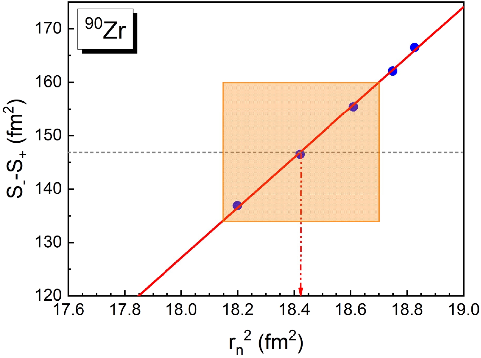
      Figure 2.  (color online) Calculated S_--S_+ values as a function of mean-square radii of the neutrons. The results are calculated with SAMi-J interactions and denoted as blue symbols.

      The neutron skin thickness is sensitive to the density dependence of the symmetry energy [59]; it is seen that the connection between \Delta r_{np} and the slope parameter L of the nuclear symmetry energy is approximately linear. Using the relationship between the nuclear symmetry energy J (its slope parameter L) and the neutron skin thickness \Delta r_{np} extracted presently, we can further place restrictions on J (L). As seen in Fig. 3, the correlation between J and \Delta r_{np} is shown in the upper panel of the figure, while the lower panel presents the connection between L and \Delta r_{np} ; the gray short-dashed lines together with shaded boxes represent the constrained neutron skin thickness of ^{90} Zr. The fitting lines are shown as well. Many studies have discussed this kind of linear relationship, and it is also shown clearly in Fig. 3. The weighted average of J in Fig. 3 (a) is given as J = 29.2 \pm 2.6\; \mathrm{MeV}. Compared with the symmetry energies obtained from other studies, the value of J in the present work is slightly smaller, but generally it still matches with other values.

      Figure 3.  (color online) Correlations between the neutron skin thicknesses \Delta r_{np} of ^{90} Zr and symmetry energies as well as the slope parameters given by SAMi-J interactions in this work.

      Finally, we discuss the slope parameter L. It can be found in Fig. 3 (b) that the correlation between L and \Delta r_{np} is approximately linear. We also constrain the value of L by the present \Delta r_{np} of ^{90} Zr, so the slope parameter L is given as L = 53.3 \pm 28.2\; \mathrm{MeV}. The L value is comparable with the results from other methods in the literature. The recent PREX-II experiment, measuring the parity violating asymmetry A _{PV} in ^{208} Pb, results in a neutron skin thickness of ^{208} Pb as \Delta r_{np}^{208}=0.283\pm0.071 \;\mathrm{fm} [22]. The experimental data of PREX-II favor a stiff symmetry energy; the symmetry energy and the slope parameter can be constrained as J=38.1 \pm 4.1 \;\mathrm{MeV} and L=106 \pm 37 MeV [60], which systematically overestimate the current accepted limits J=31.7 \pm 3.2\; \mathrm{MeV} and L=58.7 \pm 28.1 MeV [30, 61, 62]. Our results are consistent with the current accepted values.

    IV.   SUMMARY
    • In summary, we have studied the SD _\pm strengths of ^{90} Zr using the Skyrme HF plus pn-RPA with SAMi-J interactions. It is found that the present calculations can well reproduce the experimental SD _\pm strengths. We have also calculated the sum rule S_--S_+ values for each SAMi-J interaction. Employing the model-independent sum rule, we have constrained the mean-square radii of the neutrons and the neutron skin thickness \Delta r_{np} of ^{90} Zr, obtaining \Delta r_{np}=0.083 \pm 0.032 fm, which is consistent with the results of other studies; for example, the analysis of antiprotonic atoms gives \Delta r_{np}=0.09 \pm 0.02\; \mathrm{fm} in Ref. [58]. Furthermore, the relationships between the neutron skin thickness \Delta r_{np} and nuclear symmetry energy J, as well as its slope parameter L, are used to extract information on J and L. The obtained \Delta r_{np} can place a constraint on the symmetry energy and slope parameter, giving values of J=29.2 \pm 2.6\; \mathrm{MeV} and L = 53.3 \pm 28.2 \mathrm{MeV}. To date, both the experimental SD _- and SD _+ strengths are known only for ^{90} Zr; if more experimental data for other nuclei are available in the future, more accurate information on the density dependence of symmetry energy can be obtained.

Reference (62)

目录

/

DownLoad:  Full-Size Img  PowerPoint
Return
Return