


 Abstract
 HTML
HTML Reference
 Related
 PDF
PDF


-
The Massachusetts Institute of Technology (MIT) bag model describes a hadron as a bag that contains various quarks, antiquarks, and perhaps gluons [1]. It was proposed to reconcile two different ideas behind quantum chromodynamics (QCD) with a single parameter, the bag radius (R), as follows:
● Because of their asymptotic freedom, quarks move freely inside the bag.
● Quarks are not allowed to penetrate the bag because of the QCD confinement.
Expressing the ideas mathematically, we start with the free Dirac equations given by
$ \begin{array}{*{20}{l}} ({\rm i} \not {\partial } -M_q)\psi_q (x) = 0\,,\; \; \; \; \; {\rm{ in }}\; r<R \,, \end{array} $

(1) along with the boundary condition,
$ \begin{array}{*{20}{l}} -{\rm i} \left( \hat {x} \cdot \vec{\gamma } \right) \psi_q(x) = \psi_q(x) \,,\; \; \; \; \; {\rm{ at }}\; r = R \,, \end{array} $

(2) where
$ \psi_q $ stands for the quark wave function,$ M_q $ represents the quark mass with q being the quark flavor,$ r=|\vec{x}| $ ,$ \vec{\gamma} =( \gamma_{1} , \gamma_2, \gamma_3 ) $ , and R is the bag radius. The description is similar to the infinite square well in quantum physics. In practice, "bag" can be understood as the abbreviation for "infinite spherical well." The higher-order mass corrections can be done by taking$ \psi_q $ as an unperturbed state.Owing to its simplicity, the bag model can easily cooperate with various QCD systems. The applications range from atoms to burning stars. In nuclear physics, the bag model offers an intuitively understandable ground for studying the mass spectra [2–5] and the hypothetical objects, such as
$ \Xi_{bb} $ , glue balls, and pentaquarks [6–9]. See Ref. [10] for a historical review. In astrophysics, under the framework of the bag model, the strange stars, neutron stars, and quark cores are viewed as large bags containing countless quarks [11–15]. Despite these advances, the bag model has little application in the particle decay system, mainly because of the center of mass motion (CMM) [16–18]. This study is devoted to introducing the homogeneous bag model to provide a consistent framework to deal with the CMM.The paper is organized as follows. We provide a brief review of the MIT bag model in Sec. II, where we concentrate on the CMM problem rather than computational IV; we present a systematic framework for dealing with the CMM problem and show the numerical results of the neutron β decay and
$ \Lambda_b \to \Lambda \gamma $ . We conclude the paper in Sec. V. -
Since we only consider low-lying hadrons, the quark wave function of
$ \psi_q $ can be safely considered isotropic. Consequently, Eq. (1) with$ J_z=1/2 $ can be easily solved as$ \begin{equation} \psi_{q\uparrow} (x) =\phi_{q\uparrow}(\vec{x}) {\rm e}^{-{\rm i}E_qt}= {\rm N}\left( \begin{array}{c} \omega_{q+} j_0(p_qr) \chi_\uparrow\\ i\omega_{q-} j_1(p_qr) \hat{r} \cdot \vec{\sigma} \chi_\uparrow\\ \end{array} \right){\rm e}^{-{\rm i}E_qt}\,, \end{equation} $

(3) where
$ \phi_q(\vec{x}) $ corresponds to the spatial part of the quark wave function with$ E_q^k = \sqrt{p_q^2 +M_q^2} $ ,$ \omega_{q\pm} = \sqrt{E^k_q \pm M_q} $ , and$ p_q $ and$ E_q $ are the magnitudes of the quark 3-momentum and energy, respectively. N is the normalization constant,$ \chi_\uparrow $ and$ \chi_\downarrow $ stand for$ (1,0)^T $ and$ (0,1)^T $ , respectively, and$ j_{0,1} $ are the zeroth and first spherical Bessel functions, which are the cosine and sine functions in the spherical coordinate. In the absence of energy corrections, we have$ E_q = E_q^k $ .In analogy to the case of the infinite square well, imposing the boundary condition would quantize
$ p_q $ . Combining Eqs. (2) and (3), we find that$ p_q $ must satisfy the relation [3]:$ \begin{equation} \tan \left(p_q R\right)=\frac{p_q R}{1-m_q R-E_q^k R}\,. \end{equation} $

(4) At the massless and heavy quark limits, we obtain
$ \begin{equation} \lim\limits_{M_q R \to 0 } p_q R = 2.043, 5.396\cdots \,,\; \; \; \lim\limits_{M_q R \to \infty } p_q R = \pi\,,2\pi \cdots \,, \end{equation} $

(5) respectively, which is valid for all hadrons. These results are handy for quick estimations, as
$ M_{u,d} $ can be considered massless, whereas$ M_{c,b} $ can be considered infinite in practice. It states that the magnitude of the 3-momentum grows along with the quark mass, approaching$ \pi /R $ .At this stage, one can readily estimate the hadron masses by adding quark energies. We take the proton as an example, and the formalism can be easily generalized to other hadrons. The proton wave function is given by superposing the quark states.
$ \begin{aligned}[b] \Psi(x_1,x_2,x_3) =& \langle 0 | \hat{u}(x_1)\hat{ u}(x_2)\hat{d}(x_3) | p_B(0) \rangle \\=& \psi_u(x_1) \psi_u(x_2) \psi_d(x_3) \,, \end{aligned} $

(6) where
$ \hat{ u} $ and$ \hat{d} $ are the quark field operators, without explicitly writing down the spin-flavor and color indices, and$ |p_B(0)\rangle $ represents the proton state from the bag model, centered in the coordinate. The experimental proton charge radius of$ 0.840 $ fm [19] corresponds to$ R= 5.85 $ GeV$ ^{-1} $ in the bag model, leading to the proton and Δ masses as$ \begin{equation} M_{p, \Delta} = \frac{2.043}{5.85 } \times 3 = 1.047\; {\rm{GeV}}\,, \end{equation} $

(7) which are close to the experimental values,
$ \begin{equation} \frac{ 1 }{2} \left( M_p + M_\Delta \right)_{{\rm{EXP}}} = 1.085\; {\rm{GeV}}\,. \end{equation} $

(8) However, the neutron charge radius is essentially zero in the bag model, which is inconsistent with the experiments.
There are several mass corrections, which can be summarized as follows [3]:
● The energy of the bag is proportional to its volume, given by
$ E_V = 4\pi B R^3/3 $ , with B being the bag energy density.● The zero-point energy is considered negative empirically, given by
$ E_0 = -Z_0/R $ .● The quark-gluon interaction introduces the strong coupling constant of
$ \alpha_s $ .Here, B,
$ Z_0 $ , and$ \alpha_s $ are considered free parameters in the model. In contrast, the bag radii are determined by minimizing the hadron masses, given as [3]:$ \begin{equation} \left. \frac{\partial M_H}{\partial R}\right|_{R=R_H} = 0\,, \end{equation} $

(9) where
$ M_H $ and$ R_H $ are the mass and bag radius of H, respectively, resulting in different hadron bag radii. Typically, the baryon and meson radii are approximately$ 5 $ and$ 3 $ GeV$ {^{-1}} $ , respectively. Except for u and d, the quark masses are considered free parameters in the model, fitted to be [9]$ \begin{equation} M_s = 0.279\; {\rm{GeV}}\,,\; \; M_c =1.641\; {\rm{GeV}}\,,\; \; M_b=5.093\; {\rm{GeV}}\,, \end{equation} $

(10) which can be viewed as effective masses when the quarks swim inside the bags.
Although the mass corrections from the bag and zero-point energies are intuitively satisfactory, they are problematic under spacetime symmetry. For instance, particles at rest are invariant under space translations. How can their masses be related to a finite volume? How do the zero-point energies transform under the Lorentz boost? These problems partly stem from the fact that the description of the bag model is a semi-classical one. Quarks are quantum objects as they satisfy the Dirac equation, whereas the bag, having a definite position and a concrete boundary, is a classical object. These are the essential problems that have haunted the bag model ever since it was proposed and are closely related to the CMM. As a pioneer of quark models, it provides an excellent framework for understanding the hadrons in relativistic systems. However, it is difficult to apply to particle decay processes.
Another issue after considering the mass corrections is that we lost the ability to track the t-dependencies of the individual quarks. The best we can obtain is the t-dependency of the proton wave function, read as
$ \begin{equation} \Psi(t, \vec{x}_{1},\vec{x}_{2},\vec{x}_{3}) ={\rm e}^{-{\rm i}M_p t } \phi_u(\vec{x}_1)\phi_u(\vec{x}_2)\phi_d(\vec{x}_3)\,. \end{equation} $

(11) Here, we can no longer consider
$ t_{1,2,3} $ different as done in Eq. (6) for$ 2E^k_u + E^k_d\neq M_p $ after including the bag and zero-point energies. Due to this reason, we cannot apply a Lorentz boost to Eq. (11), which would mix up the spacetime coordinates. The problem can be traced back to the fact that the$ t=0 $ plane is not invariant under a Lorentz boost, which we will discuss in more detail in Sec. IV, in which the wave functions are spelled out in terms of the creation operators. -
We are interested in the applications of the bag model in the decay system, in which momentum eigenstates are required. In the literature, there are two methods concerning decay with the bag model. These methods have advantages but fail to achieve a consistent framework with the Poincaré symmetry. Nonetheless, they shed light on the CMM problem, which we discuss briefly.
A bag as a wave packet
The most naïve solution to explain the CMM is the wave packet approach, which treats the bag wave function as a localized wave packet. We extract the momentum states based on the Fourier analysis, which reads as
$ \begin{equation} |p ( \vec{p})\rangle ={ N}(\vec{p}) \int {\rm d}^3x \; {\rm e}^{- {\rm i} \vec{p}\cdot \vec{x}} |p_B (\vec{x})\rangle\,, \end{equation} $

(12) where the left-hand side is a proton state with
$ \vec{p} $ as the 3-momentum, leading to the quark state decomposition as$ \begin{aligned}[b] \Psi(t, \vec{x}_1,\vec{x}_2,\vec{x}_3) =&{ N}(\vec{p}) \int {\rm d}^3x {\rm e}^{-{\rm i} \vec{p}\cdot \vec{x} -{\rm i} M_p t } \phi_u(\vec{x}_1- \vec{x})\\&\times\phi_u(\vec{x}_2- \vec{x} )\phi_d(\vec{x}_3- \vec{x })\,. \end{aligned} $

(13) One of the advantages of this method is that the t-dependencies of the quark states are not required. Thus, it can easily cooperate with the bag and zero-point energies①.
The ellipsoidal bag approach
The contradiction that occurred in the wave packet approach is attributed to the fact that we cannot have a wave packet with definite energy. To solve the problem, a Lorentz boost for the bag state is needed [20–23]. Boosting Eq. (6), the wave function is read as
$ \begin{equation} \Psi ^v (x_1,x_2,x_3) = \psi^v_{u}(x_1)\psi^v_{u}(x_2)\psi^v_{d}(x_3) \end{equation} $

(14) where v is the velocity, and
$ \begin{equation} \psi_q^v(x) = S_v \psi_q(\Lambda_v^{-1} x) \,, \end{equation} $

(15) where
$ S_v $ and$ \Lambda_v $ are the Lorentz boost matrices toward the$ \hat{z} $ direction for Dirac spinors and spacetime coordinates, respectively. In this work,$ \vec{v} $ is always chosen in the$ \hat{z} $ direction, leading to$ S_v = a_+ + a_-\gamma^0\gamma^3 $ with$ a_\pm=\sqrt{\gamma\pm1} $ and$ \gamma ^{-1}= \sqrt{1-v^2} $ . In contrast to Eq. (6), the spherical bag deforms to an ellipsoid due to the Lorentz contraction, and the bag itself is moving.The t-dependencies (
$ E_q $ ) of the quark states are needed by Eq. (15). A reasonable range for the up and down quark energies is given as$ \begin{equation} \qquad\qquad\frac{1}{3} M_p<E_{u,d} < E_{u,d}^k + \frac{1}{3} \left( E_0 + E_V \right)\,, \end{equation} $

(16) or numerically
$ \begin{equation} 0.313\; {\rm{GeV}}<E_{u,d} < 0.368\; {\rm{GeV}}\,,\qquad \end{equation} $

(17) where we allocate
$ E_0 $ and$ E_V $ evenly among the quarks. Notice that Eq. (14) admits implicitly that the energies of the quarks are independent, which is false if there are interactions among them. Thus, we have$ E_{u,d} >M_p/3 $ , and Eq. (17) serves as a major uncertainty in the evaluation. Nonetheless, for processes wherein the initial and final baryons have the same velocity, the Lorentz boost is not required. Therefore, the calculation does not suffer from uncertainty.If we take Eq. (14) as a momentum eigenstate, there are a couple of requirements to be added by hand before the calculations:
● To have the same bag volume, the initial and final hadrons must be opposite in velocities.
● As the bag is moving, a specific timing for the computation has to be chosen.
The studies of the ellipsoidal bag approach are carried out in the decays with the
$ b \to c $ transition [24], where the overlapping between the heavy quarks is treated by the heavy quark symmetry. In contrast, the overlapping of the light quarks would lead to the v-dependency of the Isgur-Wise function, shown below:$ \begin{equation} \langle l_v | l_{-v}\rangle = \int {\rm d}^3\vec{x} \psi^{v\dagger }_l(0, \vec{x})\psi^{- v }_l(0, \vec{x}) = D^v_l (0) \,, \end{equation} $

(18) with
$ \begin{equation} D^v_l (\vec{x}_\Delta ) = \frac{1}{\gamma} \int {\rm d}^3 \vec{x } \phi_l^\dagger\left(\vec{x}+ \frac{1}{2} \vec{x}_\Delta \right) \phi_l \left(\vec{x}- \frac{1}{2} \vec{x}_\Delta\right) {\rm e} ^ { - 2 {\rm i} E_l\vec{v}\cdot \vec{x}} \,, \end{equation} $

(19) where l is the spectator quark in the heavy hadron transition, and
$ D^v_l(\vec{x}_\Delta ) $ is a function of both velocity and position, and where the dependence on$ \vec{ x}_\Delta $ is defined for the latter convenience. In Ref. [24], it was found that$ {\cal B}( B^0 \to D^- l^+{\nu}_l) = 2.12\ $ %, which is close to$(2.31\pm 0.10)\$ % given by the experiments [25]. Remarkably, Eq. (18) can be understood intuitively, in which$ \gamma^{-1} $ comes from the Lorentz contraction of the bag volume, while the exponential in the integral causes the damping, which is a punishment for not being at the same velocity.However, it is unarguable that both the Lorentz and translational symmetries are broken in the ellipsoidal bag approach as a specific initial frame and timing are demanded in the computation. Furthermore, Eq. (18) shows that the inner products between
$ |l_{\pm v}\rangle $ are nonzero, violating the principle of energy-momentum conservation. -
The homogeneous bag model, first proposed in Ref. [26], has been widely applied in various decay systems [27–30]. It is meant to reconcile the Poincaré symmetry and the bag model without necessarily introducing a new parameter. However, in Ref. [26], only the scalar operators were considered. In this work, we would like to generalize the formalism to the vector and tensor operators.
In the following discussion, we will construct hadron states by combining the features of the wave packet and ellipsoidal bag approaches. Note that the wave packet approach violates the Lorentz symmetry as masses depend on velocities, whereas the ellipsoidal bag approach breaks the translational symmetry as the wave functions are localized. We will show that the inconsistencies with the Poincaré symmetry are resolved in our framework. We also take the neutron β decay as an instance of the computation, as it is independent of free parameters.
Hadron wave functions
We start with a hadron state at rest. As a zero-momentum state has to distribute itself homogeneously over the space, we linearly superpose infinite bags at different locations. A proton state at rest is constructed as
$ \begin{equation} |p (\vec{p} = 0) \rangle = {\cal N}_p \int {\rm d}^3 \vec{x} | p_B(\vec{x})\rangle \,, \end{equation} $

(20) where
$ {\cal N}_H $ is the normalization constant for the hadron H. Notice that the formula is identical to Eq. (12) when$ \vec{p}=0 $ , but the idea is different. Eq. (12) is meant to extract the specific momentum component from the wave packet, whereas we are trying to build up a momentum eigenstate from infinite static bags here.For completeness, we would write down the baryon wave functions with color and spinor indices. It can be accomplished by adopting the quark creation operators given by
$ \begin{aligned}[b] |p (\vec{p}= 0 ),\uparrow \rangle =& \int [{\rm d}^3\vec{x}] \frac{1}{2\sqrt{3}} \epsilon^{\alpha \beta \gamma} u^\dagger_{a\alpha}(\vec{x}_1)d^\dagger_{b\beta}(\vec{x}_2)u^\dagger_{c\gamma}(\vec{x}_3)\\&\times \Psi_{A_\uparrow (udu)}^{abc} ( \vec{x}_1, \vec{x}_2 , \vec{x}_3 )|0\rangle \,, \end{aligned} $

(21) along with
$ \begin{aligned}[b] \Psi_{A_{\downarrow}(q_1q_2q_3)}^{abc} ( \vec{x}_1, \vec{x}_2 , \vec{x}_3 ) =& \frac{{\cal N}_H}{\sqrt{2}} \int \left [ \phi^a_{q_1\uparrow}(\vec{x}_1- \vec{x}_\Delta) \phi^b_{q_2\downarrow}(\vec{x}_2-\vec{ x}_\Delta) \right. \\ &\left. - \phi^a_{q_1\downarrow}(\vec{x}_1- \vec{x}_\Delta) \phi^b_{q_2\uparrow}(\vec{x}_2-\vec{ x}_\Delta) \right] \\&\times \phi^c_{q_3\downarrow}(\vec{x}_3- \vec{x}_\Delta) {\rm d}^3 \vec{x}_\Delta, \end{aligned} $

(22) where
$[{\rm d}^3\vec{x}]= {\rm d}^3\vec{x}_1{\rm d}^3\vec{x}_2{\rm d}^3\vec{x}_3$ , the Greek (Latin) letters stand for the color (spinor) indices, the arrows represent the spin directions of the quarks, and the Fermi statistic is guaranteed by the anti-commutation relation:$ \begin{equation} \{ q_{a\alpha}(\vec{x}) , q^{\prime \dagger }_{b\beta}(\vec{x}\,') \} =\delta_{qq'} \delta_{ab}\delta_{\alpha\beta} \delta^3\left( \vec{x} - \vec{x}\,' \right)\,. \end{equation} $

(23) For the sake of compactness, the quark operators are evaluated at
$ t=0 $ if not stated otherwise.To obtain a nonzero momentum, we have to apply the Lorentz boost
$ U_v $ on Eq. (21). Recall that the transformation rule for the quark operators is given as$ \begin{equation} U_v^{-1} q _{a \alpha } ( \vec{x} ) U_v = \left( S_v \right) _{ab} q _{b \alpha } \left( x^v\right )\equiv \left( S_v \right) _{ab} q _{ b \alpha } \left( t=-\gamma v z , x, y , \gamma z \right ) \,. \end{equation} $

(24) It states that even if we start with the operators simultaneously, we inevitably have to deal with the quark operators with timelike distances, as the quarks have different positions in the baryon at rest. The problem can be traced back to the fact that the plane
$ t=0 $ is not invariant under the Lorentz boost, which leads to unequal time among the operators. The unequal time commutators require knowledge of the dynamical details, which cannot be perturbatively calculated. To overcome the problem, we utilize$ \begin{equation} q_{a\alpha }( t, \vec{x }_i) | p (\vec{p} = 0 ) \rangle = q_{a\alpha }( 0, \vec{x }) {\rm e}^{-{\rm i}E_q t} | p (\vec{p} = 0 ) \rangle \,, \end{equation} $

(25) which stems from the fact that the quarks are energy eigenstates in the bag model, at least for the first-order approximation.
The wave functions after the Lorentz boost can be obtained by the following trick. Without loss of generality, we write the wave functions after boosting as
$ \begin{aligned}[b] U_v|p (\vec{p}= 0 ),\uparrow \rangle =& \int [{\rm d}^3\vec{x}]\frac{1}{2\sqrt{3} } \epsilon^{\alpha \beta \gamma} u^\dagger_{a\alpha}(\vec{x}_1)d^\dagger_{b\beta}(\vec{x}_2)\\&\times u^\dagger_{c\gamma}(\vec{x}_3) ( \Psi^v )_{A_\uparrow (udu)}^{abc} ( \vec{x}_1, \vec{x}_2 , \vec{x}_3 )|0\rangle \,, \end{aligned} $

(26) where
$ \Psi^v $ is a function to be determined. Note that as$ J_z $ commutes with$ U_v $ , the proton remains an eigenstate of$ J_z $ . Applying the annihilation operators, we arrive at$ \begin{aligned}[b] &\langle 0 \left| u_{a\alpha} (\vec{x}_1)d_{b\beta} (\vec{x}_2)u_{c\gamma} (\vec{x}_3) U_v \right| p (\vec{p}= 0 )\rangle \\ =&\langle 0 \left| U_v U_v ^{-1} u_{a\alpha} (\vec{x}_1)d_{b\beta} (\vec{x}_2)u_{c\gamma} (\vec{x}_3) U_v \right| p (\vec{p}= 0 )\rangle\\ =&\langle 0 \left| U_v ^{-1} u_{a\alpha} (\vec{x}_1)U_v U_v ^{-1}d_{b\beta} (\vec{x}_2)U_v U_v ^{-1}u_{c\gamma} (\vec{x}_3) U_v \right| p (\vec{p}= 0 )\rangle\\ =&\langle 0 \left| (S_v)_{aa'} u_{a'\alpha} \left( x^v_1\right )(S_v)_{bb'} d_{b'\beta} \left( x^v_2 \right )(S_v)_{cc'} u_{c'\gamma} \left( x_3^v \right ) \right| p (\vec{p}= 0 )\rangle\\ =&{\rm e}^{{\rm i}\gamma v (E_uz_1+E_d z_2 + E_u z_3)} (S_v)_{aa'}(S_v)_{bb'}(S_v)_{cc'} \\&\langle 0 \left| u_{a'\alpha} \left( \vec{x}^v_1\right ) d_{b'\beta} \left( \vec{x}^v_2 \right ) u_{c'\gamma} \left( \vec{x}_3^v \right ) \right| p (\vec{p}= 0 )\rangle\,, \end{aligned} $

(27) with
$ \vec{x}^v = (x,y,\gamma z) $ . In the third line of Eq. (27), we have shown that the vacuum is invariant under Lorentz boosts, and the fourth and fifth ones can be obtained by Eqs. (24) and (25), respectively. By comparing the first and fifth lines of Eq. (27), we deduce that$ \begin{aligned}[b] & (\Psi^v)_{A_\uparrow(udu)} ^{abc} (\vec{ x}_1,\vec{ x}_2,\vec{ x}_3)\\=&{\rm e}^{{\rm i}\gamma v (E_uz_1+E_d z_2 + E_u z_3)} (S_v)_{aa'}\\&\times(S_v)_{bb'}(S_v)_{cc'}\Psi_{A_\uparrow(udu)} ^{a'b'c'} (\vec{ x}_1^v,\vec{ x}^v_2,\vec{ x}^v_3)\,. \end{aligned} $

(28) To obtain
$ {\cal N}_p $ , we calculate the overlapping$ \begin{aligned}[b] \langle p(\vec{p}\, ') |p( \vec{p}) \, \rangle =& {\cal N}^2_p \int {\rm e}^{{\rm i} (\gamma v-\gamma'v') (E_uz_1+E_d z_2 + E_u z_3)}\\&\phi^\dagger_u(\vec{x}_1^{v'} - \vec{x}') S_v^2\phi_u(\vec{x}_1^v - \vec{x}) \\ & \phi^\dagger_d(\vec{x}_2^{v'} - \vec{x}') S_v^2\phi_d(\vec{x}_2^v - \vec{x}) \phi^\dagger_u(\vec{x}_3^{v'} - \vec{x}')\\& S_v^2 \phi_u(\vec{x}_3^v - \vec{x}) {\rm d}^3 \vec{x} {\rm d}^3\vec{x}' [{\rm d}^3\vec{x}]\,, \end{aligned} $

(29) which can be derived from Eqs. (23), (26), and (28). The spin indices have not been written down explicitly because they are irrelevant as long as the initial and final quarks are facing the same direction. We have taken
$ S_{v'}^\dagger = S_v $ by anticipating that$ v=v' $ , or the integral, vanishes. To simplify the integral, we adopt the following variables:$\vec{x}_\Delta = \vec{x} - \vec{x}'\,,\; \; \; \; \vec{x}_A = \frac{1}{2}(\vec{x}+\vec{x}')\,,\; \; \; \; \vec{x}^{ \,r}_i = \vec{x}_{i}^v - \frac{1}{2}(\vec{x}+\vec{x}')\,. $

(30) Now, the integral is given as follows:
$ \begin{aligned}[b] & \frac{{\cal N}^2_p}{\gamma^3}\int {\rm d}^3\vec{x}_\Delta {\rm d}^3 \vec{x}_A\prod_{i=1,2,3} {\rm d}^3 \vec{x}^{\,r}_{i} \phi_{q_i}^\dagger\left(\vec{x}^{ \,r}_{i} +\frac{1}{2}\vec{x}_\Delta\right)\\& S^{2}_v \phi_{q_i}\left(\vec{x}^{ \,r}_{i} -\frac{1}{2}\vec{x}_\Delta\right) {\rm e}^{{\rm i}E_{q_i}(v-v')z^r_{i}} {\rm e}^{{\rm i}E_{q_i}( v-v' )z_A } \\ =& {\cal N}^2 \gamma (2\pi)^3 \delta(\vec{p} -\vec{p}' ) \int {\rm d}^3\vec{x}_\Delta \prod_{i=1,2,3} D^0_{q_i} (\vec{x}_\Delta ) \,, \end{aligned} $

(31) where
$ (q_1,q_2,q_3) = (u,d,u) $ ,$ 1/\gamma^3 $ comes from the Jacobian in Eq. (30), and$ D_{q}^0(\vec{x}_\Delta) $ is defined in Eq. (19) with$ v=0 $ . To obtain the correct δ function, we have to demand that$ \begin{equation} M_p=\sum\limits_{i = 1,2,3} E_{q_i}\,, \end{equation} $

(32) for the integral of
$ \vec{x}_A $ , which is the main source of errors in our model. However, the range in Eq. (16) shall cover the reasonable values. The δ function can be interpreted as that the overlapping of$ D_q^0(\vec{x}_\Delta) $ for the bags with a distance$ \vec{x}_\Delta $ occurs infinite times in the integral, which is essentially a result of the translational symmetry.By taking the normalization of a momentum state as
$ \begin{equation} \langle \vec{p},\lambda_p|\vec{p}',\lambda_p' \rangle = u^\dagger_p u_p' (2\pi)^3\delta^3(\vec{p}-\vec{p}')\,, \end{equation} $

(33) where
$ u_p $ and$ \lambda_p $ are the Dirac spinor and spin of the proton, we find that$ \frac{1}{{\cal N}^2_p} = \frac{1}{\overline{u}_p u_p }\int {\rm d}^3\vec{x}_\Delta\prod_{i=1,2,3} D^0_{q_i} (\vec{x}_\Delta ) \,. $

(34) $ {\cal N}_p $ must be independent of the velocity because the Lorentz boosts are unitary for physical states. Here, our result shows that this is indeed the case in contrast to Eq. (12). The wave functions and normalization constants of other baryons can be obtained straightforwardly with trivial modifications. In Appendix A, we give the baryon wave functions at rest that are used in this work, and the evaluation of$ {\cal N}_p $ can be found in Appendix B.Here, we summarize a few steps to construct the hadron wave functions:
● We start with the hadrons at rest, where the translational symmetry is respected. At this stage, hadrons are not moving yet. Thus, we do not need to worry about the Lorentz symmetry.
● The nonzero momentum states are acquired by Lorentz boosts on the physical states, which respect both the translational and Lorentz symmetries.
Since the Poincaré symmetry is preserved in all the steps, we conclude that our approach is consistent. In the next section, we will show explicitly that the form factors do not depend on the Lorentz frame, in contrast to the wave packet and ellipsoidal approaches.
Transition matrix elements
After the hadron wave functions are constructed, the calculations of the transition matrix elements are straightforward. Here, we choose the neutron-proton transition as an example with
$ d\to u $ at the quark level. For the calculation, we adopt the Briet frame, where n and p have opposite velocities, and without loss of generality, we take$ \vec{v} \parallel \hat{z} $ . By sandwiching the quark transition operators with the hadron states, we arrive at$ \begin{aligned}[b]& \langle p (\vec{v}\,), \lambda_p | u ^ \dagger\Gamma d (0) |n (- \vec{v}\,), \lambda_n \rangle \\=& {\cal N}_{n} {\cal N}_{p} \int {\rm d}^3\vec{x}_\Delta \Gamma^{\lambda_p\lambda_n} _{ud}(\vec{x}_\Delta) \prod_{q=u,d } D^v_{q}(\vec{x}_\Delta)\,, \end{aligned} $

(35) along with
$ \begin{aligned}[b] \Gamma _{ud} ^{\lambda_p\lambda_n} (\vec{ x}_\Delta)=&\sum_{\lambda_u,\lambda_d} N^{\lambda_p\lambda_n}_{\lambda_u\lambda_d}\int {\rm d}^3\vec{x} \phi _{u{\lambda_u}}^\dagger\left(\vec{x} ^+ \right)\\&\times S_{\vec{ v}}\Gamma S_{-\vec{ v}} \phi_{d{\lambda_d}}\left(\vec{x} ^- \right) {\rm e}^{2{\rm i}(E_{u} + E_{d})\vec{ v}\cdot \vec{ x} }\,, \end{aligned} $

(36) where Γ is an arbitrary Dirac matrix and
$ \vec{x}^\pm = \vec{x}\pm \vec{x}_\Delta /2 $ . Here,$ \lambda_{u,d} \in (\uparrow,\downarrow) $ are the spins of the annihilated up and down quarks, and$ N^{\lambda_p\lambda_n}_{\lambda_u\lambda_d} $ represents the overlapping with specific$ \lambda_{p,n,u,d} $ , which can be computed by matching the LHS and RHS of Eq. (35). As the value of$ N^{\lambda_p\lambda_n}_{\lambda_u\lambda_d} $ is independent of the velocity, it can be obtained by taking$ \vec{v} = 0 $ for convenience. From the angular momentum conservation, we have that$ \begin{array}{*{20}{l}} &&N^{\lambda_p\lambda_n}_{\lambda_u\lambda_d} = 0,\; \; \; \; \; {\rm{for}}\; \; \lambda_n-\lambda_p \neq \lambda_d - \lambda_u \,. \end{array} $

(37) It states that if the baryon spin is (un)flipped by the operator, then the quark spin shall also be (un)flipped. On the other hand, by the Wiger-Eckart theorem, we have
$ \begin{equation} N^{\uparrow \uparrow}_{\lambda_u\lambda_d} = N^{\downarrow \downarrow}_{-\lambda_u-\lambda_d}\,,\; \; \; \; N^{\uparrow \uparrow}_{\uparrow\uparrow} - N^{\uparrow \uparrow}_{\downarrow\downarrow}= N^{\downarrow\uparrow}_{\downarrow\uparrow} = N^{\uparrow\downarrow}_{\uparrow\downarrow}\,. \end{equation} $

(38) Consequently, there are only two independent numbers in
$ N^{\lambda_p\lambda_n}_{\lambda_u,\lambda_d} $ , given as$ \begin{equation} N_{{\rm{nonflip}}} \equiv N^{\uparrow\uparrow}_{\uparrow\uparrow} +N^{\uparrow\uparrow}_{\downarrow\downarrow}\,,\; \; \; \; N_{{\rm{flip}}} \equiv N^{\downarrow\uparrow}_{\downarrow\uparrow}\,. \end{equation} $

(39) In the
$ n\to p $ beta decays, we have$ (N_{{\rm{nonflip}}} ,N_{{\rm{flip}}} ) = ( 1, 5/3) $ .Each term in Eq (35) has a concrete physical meaning, which can be summarized as follows:
●
$ D_{q}^v(\vec{x}_\Delta) $ are the overlapping coefficients of the spectator quarks (u and d) in the initial and final states, as found in the ellipsoidal bag approach. Note that the centers of the quark wave functions are separated by a distance of$ \vec{x}_\Delta $ ;●
$ \Gamma _{ud} ^{\lambda_p\lambda_n} (\vec{ x}_\Delta) $ is the overlapping coefficient of$ d\to u $ at quark level. Again, the centers of the bags are separated at a distance of$ \vec{x}_\Delta $ .Here, we have found that the overlapping integrals of the spectator quarks with different velocities (
$ D^v_{q} $ ) do not vanish, a feature inherited from the ellipsoidal bag approach. However, we have energy-momentum conservation when we consider the whole wave function [26]. It can be viewed as the spectator quarks being kicked by the bag, which in turn are kicked by the quark transition operators.The main ambiguity of the homogeneous bag model comes from
$ E_q $ in the exponential, as shown in Eq. (16). However, the deviations are insensitive at low velocities, as$ E_q $ is always followed by v, which does not affect the calculation for the neutron-proton transition.For the neutron β decay, the dimensionless form factors
$ F_1^{V,A} $ are defined by [31]$ \begin{aligned}[b] \langle p (\vec{v}_p) | \overline{u }\gamma^\mu d (0) |n ( \vec{v}_n ) \rangle =&\overline{u}_{p}(\vec{v}_p) \left( F^V_1(q^2) \gamma^{\mu} - F^V_2 (q^2){\rm i} \sigma^{\mu \nu} \frac{q_\nu}{ M_{n}} +F^V_3(q^2) \frac{q^{\mu}}{M_{n}} \right) u_{n}(\vec{v}_n)\,, \\ \langle p (\vec{v}_p)) | \overline{u} \gamma^\mu \gamma^5 d (0)| n (\vec{v}_n)\,) \rangle =&\overline{u}_{p}(\vec{v}_p) \left( F^A_1(q^2) \gamma^\mu - F^A_2 (q^2){\rm i} \sigma_{\mu \nu} \frac{q^\nu}{ M_{n}} +F^A_3(q^2) \frac{q^\mu}{M_{n}} \right)\gamma^5 u_{n}(\vec{v}_n)\,, \end{aligned} $

(40) where q corresponds to the 4-momentum difference of the neutron and proton, and
$ \vec{v}_n $ and$ \vec{v}_p $ are the velocities of the neutron and proton, respectively.$ F_1^V $ and$ F_1^A $ can be extracted straightforwardly after computing the transition matrix elements with$ \Gamma= 1 $ and$ \Gamma = \gamma^0\gamma^{1}\gamma_5 $ , respectively. In the model, u and d are taken as massless, and thus there is only one free parameter, R, having the length dimension. The twist is that$ F_1^{V,A} $ does not rely on the bag radius since the length dimension cannot be canceled. At the$ v \to 0 $ limit, we find that$ \begin{equation} F^V_1 = 1 \,,\; \; \; \; F^A_1 = 1.31\,, \end{equation} $

(41) which are close to the experimental value of
$ F_1^A/F_1^V = 1.27 $ . The details of the numerical evaluation can be found in Appendix B. Compared to the result of$ F_1^A/F_1^V = 1.09 $ , given previously in the bag model [3], the ratio improves significantly after considering the correction from the CMM.Notice that to compute the matrix elements, we have taken the Briet frame, where the initial and final hadrons have opposite velocities. However, in principle, it can be calculated in other Lorentz frames. For an illustration, with
$ \Gamma = \gamma^0 \gamma^\mu $ , we have$ \begin{aligned}[b] & \langle p ({v}\,), \lambda_p | \overline{u }\gamma^\mu d (0) |n (- \vec{v}\,), \lambda_n \rangle \\=&\langle p (0), \lambda_p | U_{-v}\overline{u}\gamma^\mu d (0) U_{-v} |n (0), \lambda_n \rangle\\ =& \langle p (0), \lambda_p | U^2_{-v}U_v\overline{u}\gamma^\mu d (0) U_{-v} |n (0), \lambda_n \rangle \\=& \langle p (\vec{v}\,'), \lambda_p |\overline{u} S_{v}\gamma^\mu S_{-v} d (0) |n (0), \lambda_n \rangle \\ =& \langle p (\vec{v}\,'), \lambda_p |\overline{u} (\Lambda_{-v})^\mu\, _\nu \gamma^\nu d (0) |n (0), \lambda_n \rangle \\=& (\Lambda_{-v})^\mu\, _\nu \langle p (\vec{v}\,'), \lambda_p |\overline{u} \gamma^\nu d (0) |n (0), \lambda_n \rangle \,, \end{aligned} $

(42) where
$ U_v^2 = U_{v'} $ , the use of Eq. (24) has been made in the second line and$ S_{-v} \gamma^{\mu'} S_{v} = (\Lambda_v)^{\mu'}\,_{\nu}\gamma^\nu $ in the third line. Plugging in the last equation in Eq. (40), we find that$ \begin{aligned}[b] \langle p(\vec{v}\,') | \overline{u} \gamma^\mu d(0) | n(0)\rangle =& (\Lambda^{-1}_v)^\mu\,_{\mu'} \overline{u}_{p}(\vec{v}\,') \left( F^V_1(q^2) \gamma^{\mu'} - F^V_2 (q^2){\rm i} \sigma^{\mu' \nu} \frac{q'_\nu}{ M_{n}} +F^V_3(q^2) \frac{q'^{\mu'}}{M_{n}} \right)u_{n}(0)\\ =&(\Lambda^{-1}_{v})^{\mu}\,_{\mu '} \overline{u}_{p}(\vec{v}\,)S_{-v} \left( F^V_1(q^2) \gamma^{\mu'} - F^V_2 (q^2){\rm i} \sigma^{\mu' \nu} \frac{q'_\nu}{ M_{n}} +F^V_3(q^2) \frac{q'^{\mu'}}{M_{n}} \right)S_v u_{n}(-\vec{v})\\ =& \overline{u}_{p}(\vec{v}\,) \left( F^V_1(q^2) \gamma^{\mu} - F^V_2 (q^2){\rm i} \sigma^{\mu \nu} \frac{q_\nu}{ M_{n}} +F^V_3(q^2) \frac{q^{\mu}}{M_{n}} \right) u_{n}(-\vec{v})\,, \end{aligned} $ 
(43) with
$ q'^{\mu} = (\Lambda_v)^\mu\,_\nu q^\nu $ , which are identical to$ \begin{aligned}[b] \langle p(\vec{v}) | \overline{u} \gamma^\mu d(0) | n(-\vec{v})\rangle =& \overline{u}_{p}(\vec{v} ) \Big( F^V_1(q^2) \gamma^{\mu} - F^V_2 (q^2){\rm i} \sigma^{\mu \nu} \frac{q_\nu}{ M_{n}} \\& +F^V_3(q^2) \frac{q^{\mu}}{M_{n}} \Big)u_{n}(-\vec{v})\,. \end{aligned} $

(44) Thus, the results are independent of the Lorentz frame we choose, in contrast to the ellipsoidal bag approach. We conclude that the Poincaré symmetry is recovered by combing the feature of the wave functions to be invariant under spacetime translations.
For the heavy quark transitions, we use the decay of
$ \Lambda_b \to \Lambda \gamma $ as an example, which is governed by the tensor operator of$ b\to s $ . The bag radii of Λ and$ \Lambda_b $ are approximately$ 5 $ and$ 4.6 $ GeV$ ^{-1} $ , respectively [3, 9]. We take both of them as$ 4.8 $ GeV$ ^{-1} $ to simplify the numerical calculations. In addition, we find that the results depend little on the quark masses as long as the values are reasonable. For simplicity, we use [25]$ \begin{equation} (M_s , M_b) = (0.1, 4.78)\; {\rm{GeV}}\,, \end{equation} $

(45) where
$ M_s $ and$ M_{b} $ are taken as the current and pole masses, respectively. The tensor form factors are defined as$ \begin{aligned}[b] \langle \Lambda | \overline{s} i \sigma^{\mu\nu} q_\nu \gamma_5 b| \Lambda_b\rangle =&\overline{u}_\Lambda \Big[ f_1^{T A}\left(q^2\right)\left(\gamma^\mu q^2-q^\mu q_\nu \gamma^\nu \right) / M_{\Lambda_b}\\&-f_2^{T A}\left(q^2\right) {\rm i} \sigma^{\mu \nu}q_\nu \Big]\gamma_5 \overline{u}_{\Lambda _b}\,, \end{aligned} $

(46) of which only
$ f_2^{TA} $ is relevant to the weak radiative decay. It can be calculated by taking$ \Gamma = \gamma^0 \sigma^{1\nu} q_{\nu} $ in Eq. (35) with a slight modification, as$ \begin{aligned}[b]& \langle \Lambda (\vec{v}\,), \lambda_{\Lambda} | s ^ \dagger \Gamma b (0) |\Lambda_b (- \vec{v}\,), \lambda_{\Lambda_b} \rangle \\=& {\cal N}_{\Lambda} {\cal N}_{\Lambda_b} \int {\rm d}^3\vec{x}_\Delta \Gamma^{\lambda_{\Lambda}\lambda_{\Lambda_b}} _{\lambda_s\lambda_b}(\vec{x}_\Delta) \prod_{q=u,d } D^v_{q}(\vec{x}_\Delta)\,, \end{aligned} $

(47) with
$ \begin{aligned}[b] \Gamma^{\lambda_{\Lambda}\lambda_{\Lambda_b}} _{\lambda_s\lambda_b}(\vec{ x}_\Delta)=&\sum_{\lambda_s,\lambda_b} N^{\lambda_{\Lambda}\lambda_{\Lambda_b}} _{\lambda_s\lambda_b}\int {\rm d}^3\vec{x} \phi _{s{\lambda_s}}^\dagger\left(\vec{x} ^+ \right) \\&\times S_{\vec{ v}}\Gamma S_{-\vec{ v}} \phi_{b{\lambda_b}}\left(\vec{x} ^- \right) {\rm e}^{2{\rm i}(E_{u} + E_{d})\vec{ v}\cdot \vec{ x} }\,. \end{aligned} $

(48) For
$ E_u $ in the range of Eq. (17), the form factor is found to be$ \begin{equation} f_2^{TV}\left(q^2=0\right) = 0.13 4\pm 0.034 \,, \end{equation} $

(49) leading to
$ \begin{equation} {\cal B} (\Lambda_b \to \Lambda \gamma) = ( 6.8 \pm 3.3 ) \times 10 ^{ -6} \,, \end{equation} $

(50) where the numerical evaluations of the form factors are given in Appendix B. The formalism of the branching fraction can be found in Ref. [32], given as
$ \begin{aligned}[b] {\cal B}\left(\Lambda_b \rightarrow \Lambda \gamma\right)=&\frac{\tau_{b }\alpha_{e m}}{32 \pi^4} G_{\rm F}^2 M_b^2 M_{\Lambda_b}^3\left|V_{t s} ^* V_{t b}\right|^2\left(C_{7 \gamma}^{\rm e f f}\right)^2\\&\times\left(1-\frac{M_{\Lambda}^2}{M_{\Lambda_b}^2}\right)^3 \left|f_2^{T A}\right|^2\,, \end{aligned} $

(51) where
$ \tau_b $ is the lifetime of$ \Lambda_b $ ,$G_{\rm F}$ is the Fermi constant,$ \alpha_{e m} = 1/137 $ ,$C_{7 \gamma}^{\rm e f f} =0.303$ , and$ M_b = 4.8 $ GeV. Our result of the branching ratio is consistent with that given by the experiment, i.e.,$ (7.1\pm 1.7)\times 10^{-6} $ [25]. In contrast to Eq. (41), the form factors of$ \Lambda_b \to \Lambda $ suffer large uncertainties from the quark energies since the Lorentz boost with high velocity ② is needed. Alternatively, one can fit the quark energies from the experiments, resulting in$ \begin{equation} E_{u,d}= (0.33\pm 0.01) \; {\rm{GeV}}\,, \end{equation} $

(52) which is consistent with Eq. (17) and useful for future work.
-
We have reviewed the attempts at tackling the CMM of the bag model in the literature. We have discussed the advantages of the wave packet and the ellipsoidal bag approaches and their inconsistencies with Poincaré symmetry. By combing their merits, we have proposed the framework of the homogeneous bags, which is consistent with the Poincaré symmetry. Notably, we have shown that in our framework, the dominated form factors of the neutron β decay do not depend on any free parameters and are given as
$ F_1^A/F_1^V = 1.31 $ , which is close to the experimental value of$ 1.27 $ . For the heavy quark transition, we have taken the decay of$ \Lambda_b \to \Lambda \gamma $ as an example and obtained$ {\cal B}(\Lambda_b \to \Lambda \gamma) = (6.8 \pm 3.3) \times 10^{-6} $ , which is consistent with the experimental measurement of$ (7.1 \pm 1.7 ) \times 10^{-6} $ . In conclusion, we have found that the homogeneous bag model is useful in both light and heavy quark systems. The homogeneous bag model can provide a reliable framework for the computations concerning the hadron transitions, including the form factors and the decay constants. -
We collect the baryon wave functions at rest that are used in this work:
$ \begin{aligned}[b] |p,\uparrow \rangle =& \int [{\rm d}^3\vec{x}] \frac{1}{2 \sqrt{3}} \epsilon^{\alpha \beta \gamma} u^\dagger_{a\alpha}(\vec{x}_1)d^\dagger_{b\beta}(\vec{x}_2)u^\dagger_{c\gamma}(\vec{x}_3)\\&\times \Psi_{A_\uparrow (udu)}^{abc} ( \vec{x}_1, \vec{x}_2 , \vec{x}_3 )|0\rangle \,,\\ |n ,\uparrow\rangle =& \int [{\rm d}^3\vec{x}] \frac{1}{2 \sqrt{3}} \epsilon^{\alpha \beta \gamma} u^\dagger_{a\alpha}(\vec{x}_1)d^\dagger_{b\beta}(\vec{x}_2)d^\dagger_{c\gamma}(\vec{x}_3)\\&\times \Psi_{A_\uparrow (udd)}^{abc} ( \vec{x}_1, \vec{x}_2 , \vec{x}_3 )|0\rangle \,,\\ |\Lambda,\uparrow\rangle =& \int [{\rm d}^3\vec{x}] \frac{1}{ \sqrt{6}} \epsilon^{\alpha \beta \gamma} u^\dagger_{a\alpha}(\vec{x}_1)d^\dagger_{b\beta}(\vec{x}_2)s^\dagger_{c\gamma}(\vec{x}_3)\\&\times \Psi_{A_\uparrow (uds)}^{abc} ( \vec{x}_1, \vec{x}_2 , \vec{x}_3 )|0\rangle \,,\\ |\Lambda_b ,\uparrow \rangle =& \int [{\rm d}^3\vec{x}] \frac{1}{\sqrt{6}} \epsilon^{\alpha \beta \gamma} u^\dagger_{a\alpha}(\vec{x}_1)d^\dagger_{b\beta}(\vec{x}_2)b^\dagger_{c\gamma}(\vec{x}_3)\\&\times \Psi_{A_\uparrow (udb)}^{abc} ( \vec{x}_1, \vec{x}_2 , \vec{x}_3 )|0\rangle \,. \end{aligned} \tag{A1}$

-
The calculations of the form factors are tedious. In principle, one can evaluate Eqs. (35) and (36) numerically and match them with the form factors defined in Eq. (40). However, in practice, there are many integrals, and we have to carry out some of the angular ones to evaluate the matrix elements numerically at a reasonable time by a computer program.
One important observation is that
$ D^v_{q}(\vec{x}_\Delta) $ , as defined in Eq.(19), is independent of quark spin. Only two directions ($ \vec{ v} $ and$ \vec{x}_\Delta $ ) are specified in the integral. Therefore,$ D^v_{q}(\vec{x}_\Delta) $ can only depend on their magnitudes and products,$ \begin{equation} D^v_{q}( \vec{x}_\Delta ) = D^v_{q}( r_\Delta , \cos \theta)\,, \end{equation}\tag{B1} $

where
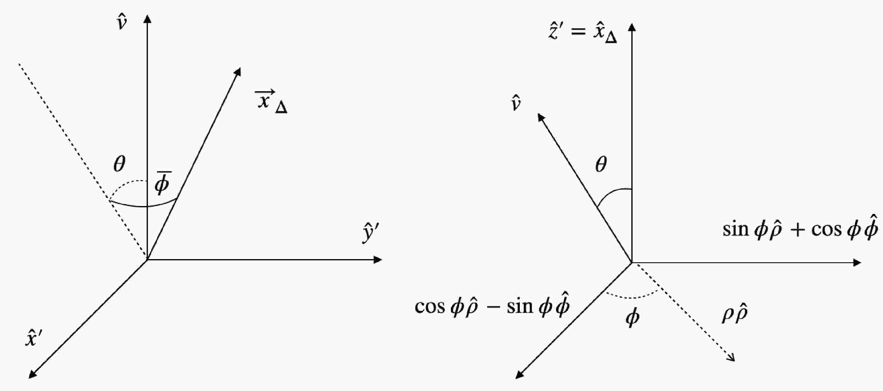
$ r_\Delta= |\vec{x}_\Delta| $ and θ is the angle between$ \vec{x}_\Delta $ and$ \vec{v} $ . Accordingly, we can rotate both$ \vec{v} $ and$ \vec{x}_\Delta $ simultaneously without affecting the numerical results. We adopt the cylindrical coordinate system$ (\rho,\phi,z') $ and use the freedom to choose$ \vec{x}_\Delta\parallel \vec{z}\,'\, $ with$ \vec{v} $ lying on the$ \hat{ \rho}\otimes \hat{z}' $ plane at$ \phi = 0 $ . To be specific, we take$ \begin{aligned}[b] \vec{x} =& \rho \hat \rho + z' \hat{ z}'\,,\; \; \; \; \vec{x}_\Delta = r_\Delta \hat{z}'\,,\\\vec{v} =& v \left( \sin \theta \cos \phi \hat{\rho} - \sin \theta \sin \phi \hat{\phi} + \cos \theta \hat z ' \right)\,, \end{aligned} \tag{B2}$

where
$ \vec{x} $ is the integration variable in Eq. (19), and the definitions of the angles are collected in Fig. 1. Plugging Eq. (B2) into Eq. (19), we arrive at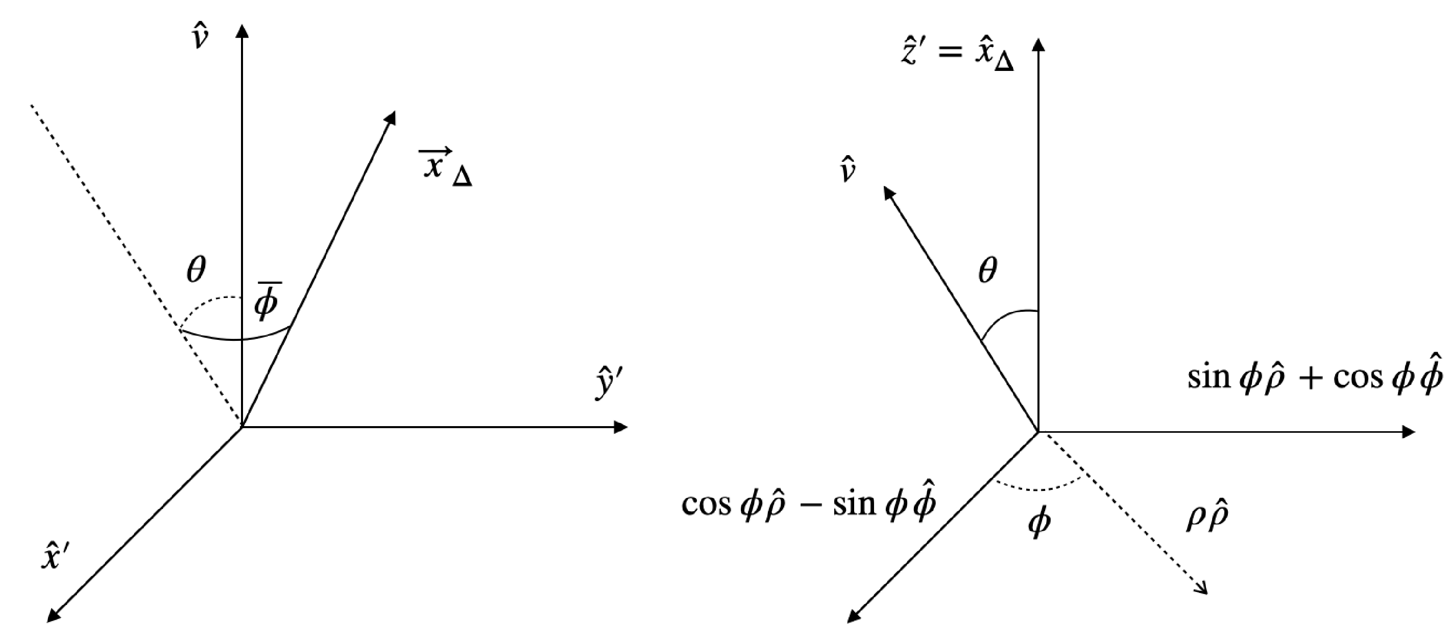
Figure 1. The definitions of the angles
$ \theta, \overline{\phi} $ and ϕ, where the right figure is the adopted cylindrical coordinate in evaluating$ {\cal D}^v_q(\vec{x}_\Delta) $ .$ \begin{aligned}[b]\\[-5pt] \gamma D^v_{q}(\vec{x}_{\Delta}) = &\int {\rm d}^3 \vec{x} \phi_{q}^\dagger \left(\vec{x}^+\right) \phi_{q} \left(\vec{x}^-\right) {\rm e}^{-2{\rm i}E_{q} \vec{ v}\cdot\vec{ x} }=\int {\rm d}^3 \vec{x} \phi_{q}^\dagger \left(\vec{x}^+\right) \phi_{q} \left(\vec{x}^-\right) {\rm e}^{-2{\rm i}E_{q} v (\sin\theta \rho \cos \phi + \cos\theta z')} \\ =& \int \rho {\rm d}\rho {\rm d}\phi {\rm d}z ' \left[ j_{0q}^+j_{0q}^- + j_{1q}^+j_{1q}^-\left( \hat{x}^+ \cdot \hat{x}^- +\frac{1}{r^+r^- } i \chi^\dagger (\vec{x}_\Delta \times \vec{x}) \cdot \vec{\sigma}\chi \right) \right]{\rm e}^{-2{\rm i}E_{q} v (\sin\theta \rho \cos \phi + \cos\theta z')}\\ =& \int \rho {\rm d}\rho {\rm d}\phi {\rm d}z ' \left( j_{0q}^+j_{0q}^- + j_{1q}^+j_{1q}^- \hat{x}^+ \cdot \hat{x}^- \right){\rm e}^{-2{\rm i}E_{q} v (\sin\theta \rho \cos \phi + \cos\theta z')}\\ =&2\pi \int \rho {\rm d}\rho {\rm d}z ' \left( j_{0q}^+j_{0q}^- + j_{1q}^+j_{1q}^- \hat{x^+} \cdot \hat{x^-} \right)J_0(2E_{q}v\sin \theta \rho)\cos \left( 2 E_{q} v \cos\theta z' \right) \,, \end{aligned} \tag{B3}$ 
where
$ J_0 $ is the zeroth Bessel function,$ \begin{equation} j_{(0,1)q}^{\pm} \equiv \omega_{q(+,-)} j_{(0,1)} ( p_{q} r^\pm) \,, \end{equation}\tag{B4} $

with
$ r^\pm = |\vec{x}^\pm| $ . Here, we have absorbed N into the overall normalization constant$ {\cal N}_{n,p} $ for convenience. Due to the finite bag radius, the integrals are bounded as$ \begin{equation} \int \rho {\rm d}\rho {\rm d} z' =\int_0^{ \sqrt{R^2-r_\Delta^2/4}} {\rm d} \rho \rho \int_{ - \sqrt{R^2-r_\Delta^2/4} + r_\Delta/2 }^{ \sqrt{R^2-r_\Delta^2/4} - r_\Delta/2 } {\rm d} z' \,. \end{equation} \tag{B5}$

For the sake of compactness, the regions of the integrations for ρ and
$ z' $ are not explicitly written down as long as there is no confusion. We have dropped$ \chi^\dagger[ (\vec{x}_\Delta \times \vec{x})\cdot \vec{\sigma}] \chi $ , since after integrating${\rm d}^3\vec{x}$ , it is proportional to$ \chi^\dagger[( \vec{x}_\Delta\times \hat{v})\cdot \vec{\sigma}] \chi $ as$ \vec{ v} $ is the only specified direction. It vanishes since we always choose the spin directions at$ \pm \hat{v} $ . In the last line of Eq. (B3), we have used$ \begin{equation} J_n(a) = \frac{1}{2\pi } \int^{\pi}_{-\pi } \exp( i n \phi- ia \sin \phi ) {\rm d} \phi \,, \end{equation}\tag{B6} $

with the integrand being an even function of
$ z' $ . Notice that Eq. (B3) is consistent with Eq. (B1) due to the fact that$ J_0(a) = J_0(-a) $ , which implies that$ J_0(2 E_{q} v \sin \theta \rho)= J_0(2 E_{q} v \sqrt{1 - \cos^2 \theta} \rho) $ . To conclude, the number of integrals in Eq. (19) is reduced to two, which significantly shortens the evaluating time.To compute the normalization constant, we take
$ v=0 $ in Eq. (B3) and arrive at$ \begin{aligned}[b] D_{q}^0 (r_\Delta)=&2\pi \int \rho {\rm d}\rho {\rm d}z ' \left( j_{0q}^+j_{0q}^- + j_{1q}^+j_{1q}^- \hat{x^+} \cdot \hat{x^-} \right)\,,\\ \frac{1}{{\cal N}_{n,p}^2} =& \frac{1}{\overline{u}_{n,p} u _{n,p}}\int 4\pi r_\Delta^2 {\rm d} r_\Delta \left( D_u^0(r_\Delta)\right) ^3 \,, \end{aligned}\tag{B7} $

where we employ the isospin symmetry
$ D_u^v = D_d^v $ .Now we turn our attention to
$ \Gamma_{ud}^{\lambda_p\lambda_n}(\vec{x}_\Delta) $ . From Eq. (B3), we find that$ D^v_{q}(\vec{x}_\Delta) $ is an even function of$ \vec{x}_\Delta $ . Thus, we can drop the odd terms regarding$ \vec{x}_\Delta $ in$ \Gamma_{ud}^{\lambda_p\lambda_n}(\vec{x}_\Delta) $ . In this work, we use$ \Gamma = 1 $ and$ \Gamma = \gamma^0 \gamma^1\gamma_5 $ as examples. To evaluate$ \Gamma=1 $ , we take$ \lambda_n =\lambda_p = \uparrow $ in Eqs. (35) and (36), resulting in$ \begin{aligned}[b] \Gamma _{ud} ^{\uparrow \uparrow } (\vec{ x}_\Delta)=& N_{\uparrow\uparrow}^{\uparrow\uparrow}\int {\rm d}^3\vec{x} \phi _{u{\uparrow}}^\dagger\left(\vec{x} ^+ \right) \phi_{d{\uparrow}}\left(\vec{x} ^- \right) {\rm e}^{2{\rm i}E_{{\rm{di}}}\vec{ v}\cdot \vec{ x} }\\& + N_{\downarrow\downarrow}^{\uparrow\uparrow}\int {\rm d}^3\vec{x} \phi _{u{\downarrow}}^\dagger\left(\vec{x} ^+ \right) \phi_{d{\downarrow}}\left(\vec{x} ^- \right) {\rm e}^{2{\rm i}E_{{\rm{di}}}\vec{ v}\cdot \vec{ x} } \\ =& N_{{\rm{nonflip}}} \int {\rm d}^3\vec{x} \phi _{u{\uparrow}}^\dagger\left(\vec{x} ^+ \right) \phi_{d{\uparrow}}\left(\vec{x} ^- \right) {\rm e}^{2{\rm i}E_{{\rm{di}}}\vec{ v}\cdot \vec{ x} } \\ =&2\pi \int \rho {\rm d}\rho {\rm d}z ' \left( j_{0u}^+j_{0q_d}^- + j_{1q_u}^+j_{1q_d}^- \hat{x^+} \cdot \hat{x^-} \right)J_0(\delta_\rho)\cos \left( \delta_z \right) \,, \\ \delta_\rho \equiv & 2 E_{{\rm{di}}} v \sin \theta \rho \,,\; \; \; \; \; \delta_z \equiv 2 E_{{\rm{di}}} v \cos \theta z' \end{aligned}\tag{B8} $

where
$ E_{{\rm{di}}}= E_{u} + E_{d} $ is the energy of the spectator quarks. Finally, we obtain$ \begin{aligned}[b] &\langle p (\vec{v}\,), \uparrow | u ^ \dagger d (0) |n (- \vec{v}\,), \uparrow \rangle \\ =& {\cal N}_{n} {\cal N}_{p} 2\pi \int^{2R}_0 r_\Delta^2 {\rm d}r_\Delta \int^{1}_{-1} {\rm d}\cos \theta \Gamma^{\uparrow\uparrow} _{ud}(r_\Delta,\cos\theta) \left( D^v_{u}(r_\Delta,\cos \theta) \right) ^2 \,. \end{aligned} \tag{B9}$

In the neutron β decay, we can safely set
$ v\to 0 $ and neglect the contributions from$ F_{2,3}^{V,A} $ . Comparing the right-hand sides of Eqs. (40) and (B9), we find$ F_1^V = 1 $ .Now we turn our attention to
$ \Gamma = \gamma^0 \gamma^1 \gamma_5 $ . The trick of Eq. (B1) cannot be applied, as Γ provides an extra direction. In the cylindrical coordinate described in Eq. (B2), we have$ \begin{aligned}[b] \Gamma = &\gamma^0 \gamma^1 \gamma_5 =\left( \begin{array}{cc} \hat{ x }' \cdot \vec{\sigma}& 0 \\ 0 & \hat{ x}'\cdot\vec{\sigma} \end{array} \right)\,,\\ \hat{x}' =& \left(- \sin \overline{\phi} \sin \phi - \cos \overline{\phi} \cos \theta \cos \phi \right)\hat{\rho}\\& +\left( \cos \overline{\phi} \cos \theta \sin \phi - \sin \overline{\phi}\cos \phi \right)+ \sin\theta \cos \overline{\phi} \hat{z}'\,, \end{aligned}\tag{B10}$

where
$ \overline{\phi} $ is the azimuthal angle between the$ \vec{v} \otimes \vec{x}' $ and$ \vec{ v}\otimes \vec{x}_\Delta $ planes. In addition, we have$ \begin{aligned}[b] \hat{x}'\cdot \vec{\sigma} \hat{v} \cdot\vec{\sigma} =& -{\rm i}\hat{y}' \cdot \vec{\sigma}\,,\; \; \; \; \; \hat{y}'\cdot \vec{\sigma} \hat{v}\cdot\vec{\sigma} = {\rm i} \hat{x}'\cdot\vec{\sigma}\\ \hat{y}' =& \left( \cos \overline{\phi} \sin \phi - \sin \overline{\phi} \cos \theta \cos \phi \right)\hat{\rho} \\&+\left( \sin \overline{\phi} \cos \theta \sin \phi + \cos \overline{\phi}\cos \phi \right)+ \sin\theta \sin \overline{\phi} \hat{z}'\,. \end{aligned} \tag{B11}$

Here,
$ \hat{x}' $ and$ \hat{y}' $ point toward the x and y directions, respectively, when we choose$ \vec{ v}\parallel \hat{z} $ with the cartesian coordinate system (see Fig. 1). We define$ \begin{aligned}[b] {\cal G} \equiv & \gamma^0\gamma^1 \gamma_5 S_{-v}^2 = \left( \begin{array}{cc} \hat{ x }' \cdot \vec{\sigma}& 0 \\ 0 & \hat{ x}'\cdot\vec{\sigma} \end{array} \right) \left( \begin{array}{cc} \gamma & -\gamma \vec{v}\cdot \vec{\sigma} \\ -\gamma \vec{v}\cdot \vec{\sigma} &\gamma \end{array} \right)\\=&\gamma \left( \begin{array}{cc} \hat{ x }' \cdot \vec{\sigma}& {\rm i} v \hat{y}'\cdot \vec{\sigma} \\ {\rm i} v \hat{y}'\cdot \vec{\sigma} & \hat{ x}'\cdot\vec{\sigma} \end{array} \right)\,. \end{aligned} \tag{B12}$

To calculate Eq. (36), we choose
$ (\lambda_n,\lambda_p) =( \uparrow, \downarrow) $ , which results in$ \begin{aligned}[b] \Gamma _{ud} ^{\downarrow \uparrow} (\vec{ x}_\Delta) =& {\cal N}_{{\rm{flip}}}\int {\rm d}^3\vec{x} {\cal I}(\vec{x}_\Delta) {\rm e}^{2{\rm i}(E_{u} + E_{d})\vec{ v}\cdot \vec{ x} }\,,\\ {\cal I} (\vec{x}_\Delta) \equiv& \phi _{u{\downarrow}}^\dagger\left(\vec{x} ^+ \right) {\cal G} \phi_{d{\uparrow}}\left(\vec{x} ^- \right) \\ =& \left( \begin{array}{cc} j_{0u}^+ \chi ^\dagger_\downarrow & -ij_{1u}^+ \hat{x}^+\cdot\vec{\sigma}\chi ^\dagger_\downarrow \end{array} \right) {\cal G} \left( \begin{array}{c} j_{0d}^- \chi_\uparrow\\ ij_{1d}^- \hat{x}^-\cdot\vec{\sigma}\chi _\uparrow \end{array} \right)\,, \end{aligned} \tag{B13}$

where we have used Eqs. (37) and (39) along with
$ S_v \gamma^0\gamma^ 1 \gamma_5 = \gamma^0\gamma^ 1 \gamma_5 S_{-v} $ . The integrand$ {\cal I} $ can be further simplified by noting$ \begin{aligned}[b] &\chi^\dagger_\downarrow \chi_\uparrow =0\,,\; \; \; \; \chi_\downarrow ^\dagger \vec{\sigma }\chi_\uparrow = \hat{x}' + {\rm i} \hat{y}'\,,\\ &\sigma_i\sigma_j\sigma_k = {\rm i} \epsilon_{ijk} + \delta_{jk} \sigma_i - \sigma_j \delta_{ik} + \delta_{ij} \sigma_k \,, \end{aligned}\tag{B14} $

leading to
$ \begin{aligned}[b] & \frac{1}{2}\left( {\cal I}(\vec{x}_\Delta) + {\cal I }(-\vec{x}_\Delta) \right) = {\gamma } ({\cal I}_1 + v {\cal I}_2 +{\cal I}_3) \,,\\ & {\cal I}_1 ={\cal J}_{00}\,,\; \; \; \; \; {\cal I}_2 =- {\rm i}\left[{\cal J}_{01} \hat{v}\cdot \hat{x}^- +{\cal J}_{10} \hat{v}\cdot \hat{x}^+\right]\,,\\ &{\cal I}_3 = {\cal J}_{11} ( 2 \hat{x}^+\cdot\hat{x}' \hat{x}^- \cdot \hat{x}' + {\rm i} \hat{x}^+ \cdot\hat{y}' \hat{x}^- \cdot\hat{x}' \\&\quad\quad + {\rm i} \hat{x}^- \cdot\hat{y}' \hat{x}^+ \cdot\hat{x}' - \hat{x}^+ \cdot\hat{x}^- )\,, \end{aligned} \tag{B15}$

where
$ \chi_\uparrow $ and$ \chi_\downarrow $ stand for the quark spins pointing toward the$ \hat{v} $ and$ -\hat{v} $ directions, respectively, and the first line of Eq. (B15) is because we only consider the even part of the integrand with regard to$ \vec{x}_\Delta $ . For the sake of compactness, we have defined$ \begin{equation} {\cal J}_{nm} \equiv \frac{1}{2}\left( j_{n u}^+ j_{m d}^- + j_{m u}^- j_{n d}^+\right)\; \; \; \; {\rm{for}}\; \; n,m\in \{ 0, 1 \} \,. \end{equation}\tag{B16} $

$ {\cal J}_{nm} $ depends only on$ \rho\,,\; z' $ , and$ r_\Delta $ in the cylindrical coordinates described in Eq. (B2), with the following property:$ {\cal J}_{nm}(\rho , - z' ,r_\Delta ) = {\cal J}_{mn}(\rho , z' ,r_\Delta )\,. \tag{B17} $

Accordingly, we find that
$ {\cal J}_{00} $ and$ {\cal J}_{11} $ are even functions of$ z' $ , whereas$ {\cal J}_{01}/r^+ \pm {\cal J}_{10}/r^- $ are even and odd, respectively.With Eq. (B2), the integrals of
$ {\cal I}_1 $ and$ {\cal I}_2 $ can be computed straightforwardly, similar to Eq. (B3), given as$ \begin{aligned}[b]\\[-5pt]\int {\rm d}^3\vec{x} {\cal I}_1 {\rm e}^{2{\rm i}E_{{\rm{di}}}\vec{ v}\cdot \vec{ x} } =&2\pi \int \rho {\rm d}\rho {\rm d}z ' {\cal J}_{00} J_0(\delta_\rho)\cos \left( \delta_ z \right) \,,\\ \int {\rm d}^3 \vec{x} {\cal I}_2 {\rm e}^{2{\rm i}E_{{\rm{di}}}\vec{ v}\cdot \vec{ x} } =&2\pi \int \rho {\rm d}\rho {\rm d}z' \Bigg[ \left( \frac{{\cal J}_{10}}{r^+} - \frac{{\cal J}_{01}}{r^-} \right)\frac{r_\Delta}{2} \cos \theta J_0 (\delta_\rho) \sin (\delta_z) \\ &+ \left( \frac{{\cal J}_{10}}{r^+}+ \frac{{\cal J}_{01}}{r^-} \right)\Big( \cos \theta z J_0(\delta_\rho) \sin \left( \delta_z \right) + \sin \theta \rho J_1(\delta_\rho) \cos \left( \delta_z \right) \Big)\Bigg] \,. \end{aligned} \tag{B18}$ 
However, from Eq. (B15), we see that
$ {\cal I}_3 $ depends also on the azimuthal angle$ \overline{\phi} $ . To compute$ \begin{equation} \int {\rm d}r_\Delta {\rm d} \cos \theta {\rm d} \overline{\phi}\int {\rm d}^3\vec{x} {\cal I}_3 {\rm e}^{2{\rm i}E_{{\rm{di}}}\vec{ v}\cdot \vec{ x} }\prod_{q=u,d } D^v_{q}(r_\Delta, \cos \theta)\,, \end{equation} \tag{B19}$

we interchange the order of the integrals of
$\int {\rm d}\overline{\phi}$ and$\int {\rm d}^3\vec{x}$ . In addition, we make use of the fact that$ D_{q}^v $ are independent of$ \overline{\phi} $ , leading to$ \begin{aligned}[b]\\[-5pt]&\int {\rm d} \overline{\phi}\int {\rm d}^3\vec{x} {\cal I}_3 {\rm e}^{2{\rm i}E_{{\rm{di}}}\vec{ v}\cdot \vec{ x} }\prod_{q=u,d } D^v_{q}(r_\Delta, \cos \theta) \\ =& \prod_{q_j=u,d } D^v_{q_j}(r_\Delta, \cos \theta) \int {\rm d}^3\vec{x} \int {\rm d} \overline{\phi} {\cal I}_3 {\rm e}^{2{\rm i}E_{{\rm{di}}}\vec{ v}\cdot \vec{ x} }\,. \end{aligned} \tag{B20}$

Therefore, we can first calculate the integrals of the azimuthal angles. By explicit calculations, we find
$ \begin{aligned}[b]\\[-5pt] &\int {\rm d}\phi \int {\rm d}\overline{\phi} 2 \hat{x}^+\cdot\hat{x}' \hat{x}^- \cdot \hat{x}' {\rm e}^{2{\rm i}E_{{\rm{di}}}\vec{ v}\cdot \vec{ x} } =\frac{4\pi^2 }{r^+r^-}\bigg[ \rho^2 \cos^2 \theta J_0(\delta_\rho) \cos(\delta_z) + \frac{1}{2}\rho^2 \sin^2 \theta \big( J_0(\delta_\rho) \\ &\qquad+ J_2(\delta_\rho) \big) \cos(\delta_z)+\sin^2 \theta \left( z^2 - \frac{r_\Delta^2}{4} \right)J_0 (\delta_\rho) \cos (\delta_z) + \sin(2 \theta)\rho z J_1(\delta_\rho) \sin(\delta_z) \bigg]\,,\\ &\int {\rm d}\phi \int {\rm d}\overline{\phi} \left( \hat{x}^+\cdot\hat{x}' \hat{x}^- \cdot \hat{y}' + \hat{x}^+\cdot\hat{y}' \hat{x}^- \cdot \hat{x}' \right) {\rm e}^{2{\rm i}E_{{\rm{di}}}\vec{ v}\cdot \vec{ x} } = 0 \,, \\ &\int {\rm d}\phi \int {\rm d}\overline{\phi} \hat{x}^+\cdot \hat{x}^- {\rm e}^{2{\rm i}E_{{\rm{di}}}\vec{ v}\cdot \vec{ x} } = \frac{4\pi^2 }{r^+r^-}\left( \rho^2 + z^2 - \frac{r_\Delta^2}{4} \right) J_0(\delta_\rho) \cos (\delta_z )\,. \end{aligned} \tag{B21}$ 
We define
$ \begin{equation} {\cal I}_3' \equiv \frac{1}{2\pi} \int {\cal I}_3 {\rm d} \overline{\phi}\,, \end{equation} \tag{B22}$

of which
$ {\cal I}_3' $ is independent of$ \overline{\phi} $ . Effectively, one can substitute$ {\cal I}_3 ' $ for$ {\cal I}_3 $ without affecting the numerical results. Collecting Eqs. (15) and (21), we arrive at$ \begin{aligned}[b] \\[-5pt] \int {\rm d}^3 \vec{x} {\cal I}_3' {\rm e}^{2{\rm i}E_{{\rm{di}}}\vec{ v}\cdot \vec{ x} } =&2\pi \int \rho {\rm d}\rho {\rm d}z' \frac{{\cal J}_{11}}{r_-r_+} \bigg\{ \Big[ \left( \frac{r_\Delta^2}{4} -z^2 \right)- \frac{1}{2}\rho ^2 \sin^2 \theta \Big] \\ &\times J_0(\delta_\rho) \cos(\delta_z) +\frac{1}{2} \rho^2 \sin^2 \theta J_2(\delta_\rho) \cos (\delta_z) + \rho z \sin (2\theta ) J_1(\delta_\rho ) \sin(\delta_z) \bigg\}\,, \\\end{aligned}\tag{B23} $ 
where we have utilized the fact that
$ {\cal J}_{nm} $ is independent of ϕ. Finally, taking all into account, we have$ \begin{aligned}[b] \langle p (\vec{v}\,), \downarrow | \overline{ u} \gamma^1 \gamma_5 d (0) |n (- \vec{v}\,), \uparrow \rangle =& \frac{5}{3}{\cal N}_n^2\int {\rm d}^3 \vec{x}_\Delta\int {\rm d}^3\vec{x} {\cal I} {\rm e}^{2{\rm i}E_{{\rm{di}}} \vec{ v}\cdot \vec{ x} }\big( D_u^v (\vec{x}_\Delta) \big)^2\\ =& \gamma \frac{5}{3}{\cal N}_n^2\int {\rm d}^3 \vec{x}_\Delta\int {\rm d}^3\vec{x}\left( {\cal I}_1 +{\cal I}_2 +{\cal I}_3' \right) {\rm e}^{2{\rm i}E_{{\rm{di}}} \vec{ v}\cdot \vec{ x} }\big( D_u^v (\vec{x}_\Delta) =1.31 \overline{u}_p u _n, \end{aligned} \tag{B24}$

where the last equation is numerically evaluated by collecting Eqs. (B18) and (B23), and taking
$ v\to 0 $ . Comparing it to Eq. (40), we find that$ F_1^A=1.31 $ , which is the desired result.On the other hand, the tensor form factors can be obtained directly through the substitutions
$ \begin{aligned}[b] (d,u)\to (b,s)\,,\; \; \; {\cal G} \to \left( \begin{array}{cc} -q_0\hat{x}' \cdot \vec{\sigma} &{\rm i} q_3 \hat{y}' \cdot \vec{\sigma} \\ -q_3 {\rm i} \hat{y}' \cdot \vec{\sigma} &q_0 \hat{x}' \cdot \vec{\sigma} \end{array} \right)\,,\end{aligned} $

$ \begin{aligned}[b] {\cal I} \to -q_0{\cal I}_1 + q_3 {\cal I}_2 '+ q_0{\cal I}_3' \, \end{aligned}\tag{B25} $

with
$ {\cal I}_2 ' =- i\frac{1}{2} \left[ (j_{0s}^+ j_{1b}^- - j_{1s}^-j_{0b}^+ )\hat{v}\cdot \hat{x}^- - (j_{1s}^+j_{0b}^- - j_{0s}^-j_{1b}^+)\hat{v}\cdot \hat{x}^+\right] \tag{B26}$

in Eq. (B13). Note that
$ {\cal N}_{{\rm{flip}}} = 1 $ for$ \Lambda_b \to \Lambda $ .
Center of mass motion in bag model
- Received Date: 2022-08-21
- Available Online: 2023-01-15
Abstract: Despite its success with mass spectra, the reputation of the bag model has been marred by embarrassment of the center of mass motion. It leads to severe theoretical inconsistencies. For instance, the masses and the decay constants would no longer be independent of the momentum. In this work, we provide a systematic approach to resolving this problem. Our framework can consistently compute the meson decay constants and baryon transition form factors. Notably, the form factors in the neutron β decays do not depend on any free parameters and are determined to be


 DownLoad: