


 Abstract
 HTML
HTML Reference
 Related
 PDF
PDF


-
Triply heavy baryons are systems of great theoretical interest, since they may help us to better understand the interaction among heavy quarks in an environment free of valence light quarks [1]. The challenge is to explain the structure and properties of such baryons from a theoretical perspective. It is expected that the potential models would be useful to gain important insights into understanding how baryons are put together from quarks. The three-quark potential is one of the most important inputs of the potential models and also key to understanding the quark confinement mechanism in baryons [2].
The interest in studying the interquark potential for a three-quark system has a long history due to its importance in the spectroscopy of baryons. It is also interesting to investigate how the three-quark potential is different from or the same as the two-body quark-antiquark potential. The first studies date back to the mid '80s [3, 4] and after more than a decade a new phase of research started around the year 2000, which continues to date [5–9]. In particular, the three-quark potential has been widely investigated in the lattice QCD [10–23]. In the SU(3) quenched lattice QCD, 3-quark potentials are found to be well reproduced by
$ V_{3 {{Q}}}\left({\boldsymbol{r}}_{1}, {\boldsymbol{r}}_{2}, {\boldsymbol{r}}_{3}\right)=\sigma_{3 {{Q}}} L_{\min }-\sum\limits_{i<j} \frac{A_{3 {{Q}}}}{\left|{\boldsymbol{r}}_{i}-{\boldsymbol{r}}_{j}\right|}+C_{3 {{Q}}}. $

(1) Here,
$ {\boldsymbol{r}}_{1}, {\boldsymbol{r}}_{2} $ , and$ {\boldsymbol{r}}_{3} $ are the positions of the three quarks, and$ L_{\min } $ is the minimum flux-tube length connecting the three quarks. The strength of quark confinement is controlled by the string tension$ \sigma_{3 {{Q}}} $ of the flux tube. The form of Eq. (1) is called the Y ansatz. These functional forms (1) indicate the flux-tube picture on the confinement mechanism. Valence quarks are linked by the color flux tube as a quasi-one-dimensional object [12].The difficulty in deriving quark confinement directly from QCD is due to the non-perturbative features of QCD. With the discovery of AdS/CFT correspondence, using the classical gravitational theory to solve the non-perturbative QCD problems becomes possible [24–26]. The holographic quark-antiquark potential was first studied in Ref. [27]. Then, Ref. [28] extended the quark-antiquark potential at finite temperature. In Refs. [29–32], a deformed factor was introduced to reproduce the Cornell potential of the quark-antiquark pair. After that, the quark-antiquark potential in extreme conditions was investigated in Refs. [33–40].
Recently, effective multi-quark potential models from holography have been proposed by Oleg Andreev at vanishing temperature and chemical potential [2, 41–46]. As we know, an environment of high temperature and density is formed in relativistic heavy-ion collision experiments [47,48]. Based on the above discussion, we recently studied the doubly heavy baryon at finite temperature from holography [49]. In this paper, we continue the previous work and investigate the potential energy of the triply heavy baryon at finite temperature and chemical potential.
The remaining parts of this paper are organized as follows. In Sec. II, we review the quark-antiquark potential and introduce the calculation of the three-quark potential. In Sec. III, we present the numerical results and compare the quark-antiquark potential with the three-quark potential. A summary and conclusion are given in Sec. IV.
-
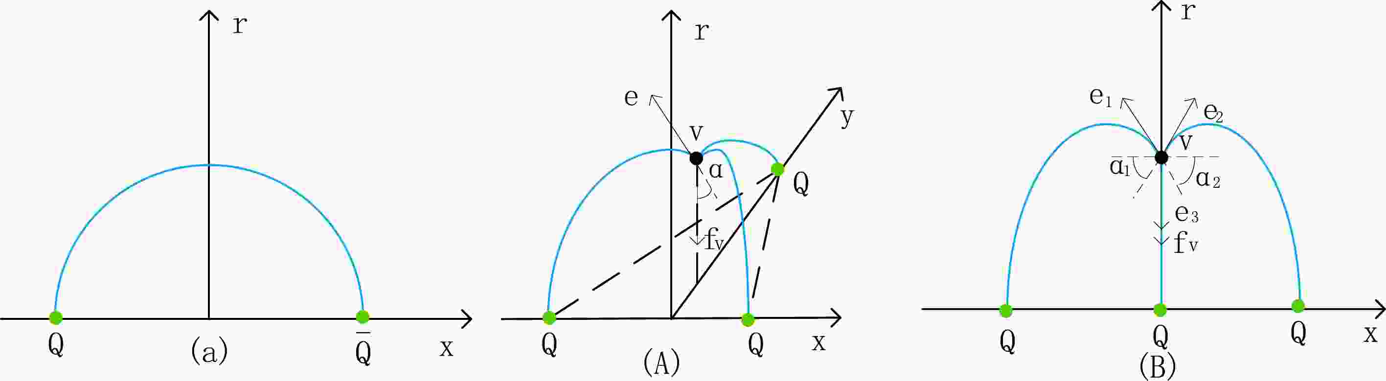
In this section, we first briefly review the calculation of quark-antiquark potential at finite temperature and chemical potential. Then, we extend the calculation to the case of the three-quark potential. The possible configurations of the quark-antiquark pair and triply heavy baryon are shown in Fig. 1. Since the ground state is dominated by the most symmetric string configuration [43], we will focus on the symmetric configurations in this paper. The study of various asymmetric configurations for QQQ is an interesting topic, which we may leave for future work.

Figure 1. (color online) String configurations for the
${Q}\bar{Q}$ and QQQ systems. The heavy quarks are at the vertices of the equilateral triangle for QQQ. (A) and (B) are different configurations for QQQ. -
Despite the fact that the deformed AdS-RN metric is not a self-consistent solution of the Einstein equation, we can still gain some insights into problems for which there are no predictions from phenomenology and the lattice. Besides, the results provided by this model on the quark-antiquark and three-quark potentials are consistent with the lattice calculations at vanishing temperature [2]. Moreover, analytic formulas can be obtained at vanishing temperature in this model. The deformed AdS-RN metric [2, 29] is given by
$ \begin{aligned}[b] {\rm d} s^{2}={\rm e}^{s r^{2}} \frac{R^{2}}{r^{2}}\left[f(r) {\rm d} t^{2}+ {\rm d} \vec{x}^{2}+f^{-1}(r) {\rm d} r^{2}\right] \end{aligned} $

$ \begin{aligned}[b] f(r)=1-\left(\frac{1}{r_{h}^{4}}+q^{2} r_{h}^{2}\right) r^{4}+q^{2} r^{6}. \end{aligned} $

(2) Here, q is the black hole charge, and
$ r_{h} $ is the position of the black hole horizon. The Hawking temperature of the black hole is defined as$ T=\frac{1}{4 \pi}\left|\frac{{\rm d} f}{{\rm d} r}\right|_{r=r_{h}}=\frac{1}{\pi r_{h}}\left(1-\frac{1}{2} Q^{2}\right), $

(3) where
$ Q=q r_{h}^{3} $ and$ 0 \leq Q \leq \sqrt{2} $ . The relation between the parameters in the deformed AdS-RN metric and the chemical potential can be obtained. It is observed that, on dimensional grounds, the low r behavior of the bulk gauge field$ A_0(r) $ is$ A_0(r) = \mu - \eta r^2 $ with$ \eta = \kappa q $ and κ is a dimensionless parameter. Together with the condition that$ A_0 $ vanishes at the horizon$ A_0(r_h) = 0 $ and$ A_{0}(0)=\mu $ , we can determine a relation between μ and the black-hole charge q:$ \mu= q \kappa r_h^2 = \kappa \frac{Q}{r_{h}}, $

(4) and we fix the parameter κ to 1 in this paper. According to the AdS/CFT dictionary, μ is the baryon number chemical potential. Thus, we can get
$ \begin{aligned}[b] f(r)=&1-\left(\frac{1}{r_{h}^{4}}+\frac{\mu^{2}}{r_{h}^{2}}\right) r^{4}+\frac{\mu^{2}}{r_{h}^{4}} r^{6}, \\ T=&\frac{1}{\pi r_{h}}\left(1-\frac{1}{2} \mu^{2} r_{h}^{2}\right),\\ A_{0}(r)=&\mu-\mu \frac{r^{2}}{r_{h}^{2}}. \end{aligned} $

(5) The quark-antiquark pair is connected by a U-shaped string in the confined phase. If we choose the static gauge
$ \xi^{1}=t $ and$ \xi^{2}=r $ , then the boundary conditions for$ x(r) $ become$ x^{(1)}(0)=-\frac{L}{2}, ~~ x^{(2)}(0)=\frac{L}{2},~~ x^{(i)}=0. $

(6) Using the static gauge
$ t=\tau, \sigma=x $ , the Nambu-Goto action of the U-shape string is$ S=\frac{1}{2 \pi \alpha^{\prime}} \int {\rm d} \tau {\rm d} \sigma \sqrt{\operatorname{det} g_{\alpha \beta}}, $

(7) with
$ g_{\alpha \beta}=G_{\mu v} \frac{\partial x^{\mu}}{\partial \sigma^{\alpha}} \frac{\partial x^{v}}{\partial \sigma^{\beta}}, $

(8) where
$ X^{\mu} $ and$ G_{\mu v} $ are the target space coordinates and the metric, respectively, and$ \sigma^{\alpha} $ with$\alpha =0, 1 $ parameterizes the worldsheet. Combining Eq. (7) and Eq. (2), we can get$ S= \frac{g}{T} \int_{-\frac{L}{2}}^{\frac{L}{2}} {\rm d} x \frac{{\rm e}^{s r^{2}}}{r^{2}} \sqrt{f(r)+\left(\partial_{x} r\right)^{2}}. $

(9) We choose the model parameters as follows:
$ g=\dfrac{R^{2}}{2 \pi a^{\prime}} $ . Now we set$w(r)=\dfrac{{\rm e}^{s r^{2}}}{r^{2}}$ and identify the Lagrangian as$ {\cal{L}}=w(r) \sqrt{f(r)+\left(\partial_{x} r\right)^{2}} $

(10) and
$ {\cal{L}}-r^{\prime} \frac{\partial{\cal{L}}}{\partial r^{\prime}}=\frac{w(r) f(r)}{\sqrt{f(r)+\left(\partial_{x} r\right)^{2}}}=\rm constant. $

(11) Using the conservation of energy, we have
$\dfrac{w(r) f(r)}{\sqrt{f(r)+\left(\partial_{x} r\right)^{2}}}= w\left(r_{0}\right) \sqrt{f\left(r_{0}\right)}$ at the maximum point$ r_{0} $ of the U-shape string. Thus, we get$ \partial_{r} x=\sqrt{\frac{w^{2}\left(r_{0}\right) f^{2}\left(r_{0}\right)}{w^{2}(r) f^{2}(r) f\left(r_{0}\right)-w^{2}\left(r_{0}\right) f^{2}\left(r_{0}\right) f(r)}}. $

(12) Finally, the separation length of the quark-antiquark pair can be expressed as
$ \begin{aligned}[b] L=&2 \int_{0}^{r_{0}} \partial_{r} x {\rm d} r\\ =&2 \int_{0}^{r_{0}} \sqrt{\frac{w^{2}\left(r_{0}\right) f^{2}\left(r_{0}\right)}{w^{2}(r) f^{2}(r) f\left(r_{0}\right)-w^{2}\left(r_{0}\right) f^{2}\left(r_{0}\right) f(r)}} {\rm d} r. \end{aligned} $

(13) Considering
$ E = T S $ , the regularized potential energy is$ \begin{aligned}[b]\\[-6pt] E = 2 g \int_{0}^{r_{0}} \left(w(r) \sqrt{1+f(r) \frac{w^{2}\left(r_{0}\right) f^{2}\left(r_{0}\right)}{w^{2}(r) f^{2}(r) f\left(r_{0}\right)-w^{2}\left(r_{0}\right) f^{2}\left(r_{0}\right) f(r)}} -\frac{1}{r^{2}} \right){\rm d} r-2 \frac{g}{r_{0}}. \\ \end{aligned} $ 
(14) In our model, there is a dynamic wall in the confined phase. The string of the quark-antiquark pair cannot go beyond the wall and the system is in the confined phase. In the deconfined phase, the dynamic wall disappears and the quark-antiquark pair can melt. Thus, we discuss the small black hole/large black hole phases that correspond to the specious-confined phase/deconfinement phases in our model. Then, the metric is valid in these different phases. More discussions can be found in Refs. [50, 51].
-
The total action of the three-quark potential is the sum of the three Nambu-Goto actions plus the action of a vertex and boundary action
$ S_A|_{r=0} $ $ S=\sum\limits_{i=1}^{3} S_{N G}^{(i)}+S_{\rm{vert}}+3 S_{A}. $

(15) The baryon vertex is given by [49, 52]
$ S_{\rm{vert}}=\tau_{v} \int {\rm{d}} t \frac{{\rm{e}}^{-2 s r^{2}}}{r} \sqrt{f(r)}, $

(16) where
$ \tau_{v} $ is a dimensionless parameter defined by$ \tau_{v}= $ $ {\cal{T}}_{5} R \operatorname{vol}(\boldsymbol{X}) $ , and$ \operatorname{vol}(\boldsymbol{X}) $ is a volume of$ \boldsymbol{X} $ . We redefine$ {\rm{k}}=\dfrac{\tau_{v}}{3 g} $ .In the presence of a background gauge field, the string endpoints with attached quarks couple to it. Hence, the worldsheet action includes boundary terms that are given by
$ S_{A}=\mp \frac{1}{3} \int {\rm d} t A_{0}. $

(17) The minus and plus signs correspond to a quark and an antiquark, respectively.
Thus, the action can now be written as
$ \begin{aligned}[b] S=\frac{3 g}{T} \int {\rm d} x \frac{{\rm e}^{s r^{2}}}{r^{2}} \sqrt{f(r)+\left(\partial_{x} r\right)^{2}}+\frac{3 {\rm{k}} g}{T} \frac{{\rm e}^{-2 s r_{v}^{2}}}{r_{v}} \sqrt{f(r)} -\frac{A_{0}(0)}{T}. \end{aligned} $

(18) The Lagrangian as
$ {\cal{L}}=\frac{{\rm e}^{s r^{2}}}{r^{2}} \sqrt{f(r)+\left(\partial_{x} r\right)^{2}}, $

(19) and
$ {\cal{L}}-r^{\prime} \frac{\partial{\cal{L}}}{\partial r^{\prime}}=\frac{\dfrac{{\rm e}^{s r^{2}}}{r^{2}} f(r)}{\sqrt{f(r)+\left(\partial_{x} r\right)^{2}}}=\rm constant. $

(20) At the points
$ r_0 $ and$ r_v $ , we have$ \begin{aligned}[b] \frac{\dfrac{{\rm e}^{s r^{2}}}{r^{2}} f(r)}{\sqrt{f(r)+\left(\partial_{x} r\right)^{2}}}=&\frac{{\rm e}^{s r_{0}^{2}}}{r_{0}^{2}} \sqrt{f\left(r_{0}\right)} \\ \frac{\dfrac{{\rm e}^{s r_{v}^{2}}}{r_{v}^{2}} f\left(r_{v}\right)}{\sqrt{f\left(r_{v}\right)+\tan ^{2} \alpha}}=&\frac{{\rm e}^{s r_{0}^{2}}}{r_{0}^{2}} \sqrt{f\left(r_{0}\right)}. \end{aligned} $

(21) The relation of
$ r_{0}, r_{v} $ and α can be determined from the above equations. We can also obtain$ \partial_{r} x=\sqrt{\frac{\dfrac{{\rm e}^{2 s r_{0}^{2}}}{r_{0}^{4}} f^{2}\left(r_{0}\right)}{\dfrac{{\rm e}^{2 s r^{2}}}{r^{4}} f^{2}(r) f\left(r_{0}\right)-\dfrac{{\rm e}^{2 s r_{0}^{2}}}{r_{0}^{4}} f^{2}\left(r_{0}\right) f(r)}} $

(22) and
$ \frac{{\rm e}^{s r_{v}^{2}}}{r_{v}^{2}} f\left(r_{v}\right)-\frac{{\rm e}^{s r_{0}^{2}}}{r_{0}^{2}} \sqrt{f\left(r_{0}\right)} \sqrt{f\left(r_{v}\right)+\tan ^{2} \alpha}=0. $

(23) The force balance equation at the point
$ r = r_v $ is$ \boldsymbol{e_{1}+e_{2}+e_{3}+f_{v}}=0. $

(24) Here
$ \boldsymbol{e_i} $ is the string tension, and$ \boldsymbol{f_v} $ is a gravitational force acting on the vertex. The presence of this force is the main difference between string models in flat spaces and those in curved spaces. In this model,$ \boldsymbol{f_v} $ only has one non-zero component in the r-direction. A formula for this component can be derived from the action$ E_{\rm {vert }}=T \cdot S_{\rm {vert }} $ . Explicitly,$ f_{v}^{r}=-\delta E_{\rm {vert }} / \delta r $ and r is the coordinate of the vertex. Each force is given by$ \begin{aligned}[b] \boldsymbol{f}_{v}=&\left(0,0,-3 g {\rm{k}} \partial_{r_{v}} \frac{{\rm e}^{-2 s r_{v}^{2}}}{r_{v}} \sqrt{f\left(r_{v}\right)}\right) \\ \boldsymbol{e}_{{\bf{1}}}=&-g \frac{{\rm e}^{s r_{v}^{2}}}{r_{v}^{2}}\Bigg(\cos \beta \frac{f\left(r_{v}\right)}{\sqrt{f\left(r_{v}\right)+\tan ^{2} \alpha}},\\& \sin \beta \frac{f\left(r_{v}\right)}{\sqrt{f\left(r_{v}\right)+\tan ^{2} \alpha}},-\frac{1}{\sqrt{1+f\left(r_{v}\right) \cot ^{2} \alpha}}\Bigg), \end{aligned} $

(25) $ \begin{aligned}[b] \boldsymbol{e}_{2}=&-g \frac{{\rm e}^{s r_{v}^{2}}}{r_{v}^{2}}\Bigg(-\cos \beta \frac{f\left(r_{v}\right)}{\sqrt{f\left(r_{v}\right)+\tan ^{2} \alpha}}, \\& \sin \beta \frac{f\left(r_{v}\right)}{\sqrt{f\left(r_{v}\right)+\tan ^{2} \alpha}},-\frac{1}{\sqrt{1+f\left(r_{v}\right) \cot ^{2} \alpha}}\Bigg), \\ \boldsymbol{e}_{3}=&-g \frac{{\rm e}^{s r_{v}^{2}}}{r_{v}^{2}}\Bigg(0,-\frac{f\left(r_{v}\right)}{\sqrt{f\left(r_{v}\right)+\tan ^{2} \alpha}},-\frac{1}{\sqrt{1+f\left(r_{v}\right) \cot ^{2} \alpha}}\Bigg). \\ \end{aligned} $

(25) Considering the symmetry in x and y, we only need to consider the force balance in the r direction. The force balance equation leads to
$ \frac{{\rm e}^{s r_{v}^{2}}}{r_{v}^{2}} \frac{1}{\sqrt{1+f\left(r_{v}\right) \cot ^{2} \alpha}}-{ {k}} \partial_{r_{v}} \frac{{\rm e}^{-2 s r_{v}^{2}}}{r_{v}} \sqrt{f\left(r_{v}\right)}=0. $

(26) Therefore, L and E can be calculated as
$ \begin{aligned}[b] L=&\sqrt{3}\left(\int_{0}^{r_{0}} \partial_{r} x {\rm d} r+\int_{r_{v}}^{r_{0}} \partial_{r} x {\rm d} r\right)\\ =&\sqrt{3}\int_{0}^{r_{0}} \sqrt{\frac{\dfrac{{\rm e}^{2 s r_{0}^{2}}}{r_{0}^{4}} f^{2}\left(r_{0}\right)}{\dfrac{{\rm e}^{2 s r^{2}}}{r^{4}} f^{2}(r) f\left(r_{0}\right)-\dfrac{{\rm e}^{2 s r_{0}^{2}}}{r_{0}^{4}} f^{2}\left(r_{0}\right) f(r)}} d r \\& +\sqrt{3}\int_{r_{v}}^{r_{0}} \sqrt{\frac{\dfrac{{\rm e}^{2 s r_{0}^{2}}}{r_{0}^{4}} f^{2}\left(r_{0}\right)}{\dfrac{{\rm e}^{2 s r^{2}}}{r^{4}} f^{2}(r) f\left(r_{0}\right)-\dfrac{{\rm e}^{2 s r_{0}^{2}}}{r_{0}^{4}} f^{2}\left(r_{0}\right) f(r)}} {\rm d} r, \end{aligned} $

(27) $ \begin{aligned}[b] E=&3 g\Bigg(\int_{0}^{r_{0}} \frac{{\rm e}^{s r^{2}}}{r^{2}} \sqrt{1+f(r)\left(\partial_{r} x\right)^{2}}-\frac{1}{r^{2}} {\rm d} r\\&+ \int_{r_{v}}^{r_{0}} \frac{{\rm e}^{s r^{2}}}{r^{2}} \sqrt{1+f(r)\left(\partial_{r} x\right)^{2}} {\rm d} r\Bigg)\\& -\frac{3 g}{r_{0}}+3 g {\rm{k}} \frac{{\rm e}^{-2 s r_{v}^{2}}}{r_{v}} \sqrt{f\left(r_{v}\right)}+3 c-\mu. \end{aligned} $

(28) -
We continue to discuss a connected collinear configuration of the triply heavy baryon. Following the procedures in the last section, we can obtain the force balance equation
$ -2 \frac{{\rm e}^{s r_{v}^{2}}}{r_{v}^{2}} \frac{1}{\sqrt{1+f\left(r_{v}\right) \cot ^{2} \alpha}}+\frac{{\rm e}^{s r_{v}^{2}}}{r_{v}^{2}}+3k \partial_{r_{ v}} \frac{{\rm e}^{-2 s r_{v}^{2}}}{r_{v}} \sqrt{f\left(r_{v}\right)}=0. $

(29) Together with Eq. (23), the relation of
$ r_{0} $ ,$ r_{v} $ and α can be determined.$ \partial_{r} x $ in this configuration can be found in Eq. (21). Thus, we can similarly obtain the inter-quark distance$ \begin{aligned}[b] L =&\int_{0}^{r_{0}} \partial_{r} x {\rm d} r+\int_{r_{v}}^{r_{0}} \partial_{r} x {\rm d} r \\ =&\int_{0}^{r_{0}} \sqrt{\frac{\dfrac{{\rm e}^{2 s r_{0}^{2}}}{r_{0}^{4}} f^{2}\left(r_{0}\right)}{\dfrac{{\rm e}^{2 s r^{2}}}{r^{4}} f^{2}(r) f\left(r_{0}\right)-\dfrac{{\rm e}^{2 s r_{0}^{2}}}{r_{0}^{4}} f^{2}\left(r_{0}\right) f(r)}} {\rm d} r\\ & +\int_{r_{v}}^{r_{0}} \sqrt{\frac{\dfrac{{\rm e}^{2 s r_{0}^{2}}}{r_{0}^{4}} f^{2}\left(r_{0}\right)}{\dfrac{{\rm e}^{2 s r^{2}}}{r^{4}} f^{2}(r) f\left(r_{0}\right)-\dfrac{{\rm e}^{2 s r_{0}^{2}}}{r_{0}^{4}} f^{2}\left(r_{0}\right) f(r)}} {\rm d} r, \end{aligned} $

(30) and the potential energy
$ \begin{aligned}[b] E= & 2 g\Bigg(\int_{0}^{r_{0}} \frac{{\rm e}^{s r^{2}}}{r^{2}} \sqrt{1+f(r)\left(\partial_{r} x\right)^{2}} {\rm d} r\\&+\int_{r_{v}}^{r_{0}} \frac{{\rm e}^{s r^{2}}}{r^{2}} \sqrt{1+f(r)\left(\partial_{r} x\right)^{2}} {\rm d} r\Bigg) \\ &-\frac{2 g}{r_{0}}+g \int_{0}^{r_{v}} \frac{{\rm e}^{s r^{2}}}{r^{2}}-\frac{1}{r^{2}} {\rm d} r-\frac{g}{r_{v}}\\&+3 g k \frac{{\rm e}^{-2 s r_{v}^{2}}}{r_{v}} \sqrt{f({r_{v}})}+3 c-\mu. \end{aligned} $

(31) -
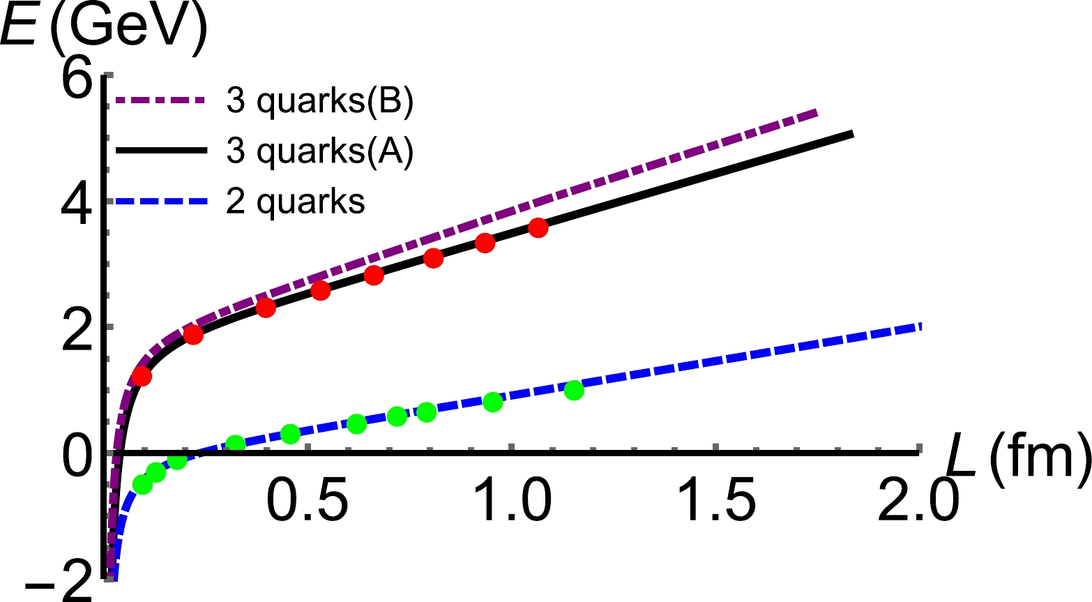
In this section, we present the results based on the discussion above. First, we use this model to calculate the potential energy of the triply heavy baryon and quark-antiquark pair in Fig. 2. The parameters are fixed by the two-quark potential and three-quark potential of lattice results at vanishing temperature and chemical potential.
Next, we investigate the behavior of separation distance at finite temperature and chemical potential in Fig. 3 and Fig. 4. The behavior of the three-quark separation distance of configuration A is similar to the quark-antiquark potential qualitatively. With increasing temperature and chemical potential, the triply heavy baryon will melt. The screening distance can be read from the maximum of the dashed line.

Figure 3. Separation distance of triply heavy baryon as a function of
$r_v$ at vanishing chemical potential. The unit of temperature is GeV.
Figure 4. Separation distance of triply heavy baryon as a function of
$r_v$ at T=0.12 GeV. The unit of μ is GeV.Then, the two-quark and three-quark potential (A) are investigated at different temperatures and chemical potentials as shown in Fig. 5. With increasing temperature and/or chemical potential, the triply heavy baryon and quark-antiquark pair dissolve. The melting temperature of the triply heavy baryon is 0.136 GeV, which is very close to the melting temperature (0.138 GeV) of the quark-antiquark pair. The screening distance
$ r_{d} $ of the triply heavy baryon is 1.14 fm at the temperature 0.14 GeV and$ r_{d} $ is 0.45 fm at the temperature 0.18 GeV in Fig. 5(a). The screening distance$ r_{d} $ of the quark-antiquark pair is 1.3 fm at the temperature 0.14 GeV and$ r_{d} $ is 0.5 fm at the temperature 0.18 GeV in Fig. 5(b). It is found that the screening distance of the quark-antiquark pair is larger than that of the triply heavy baryon. Thus, we infer that the quark-antiquark pair may be more stable than the triply heavy baryon. Similarly, we fix the temperature and study the effect of chemical potential on the three-quark potential in Fig. 6. It is found that the triply heavy baryon will also melt at large enough μ.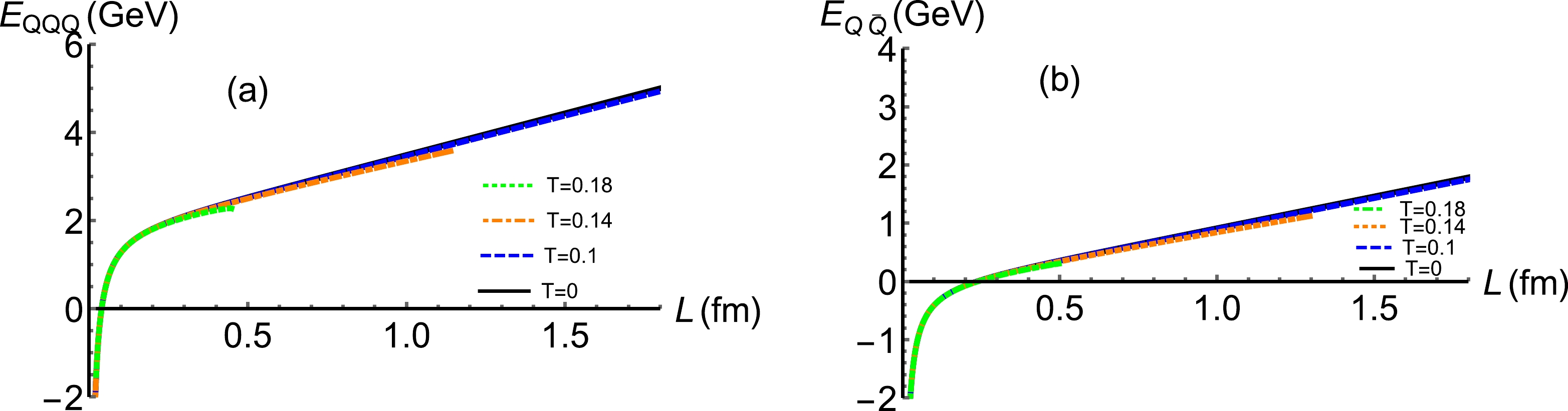
Figure 5. (color online) Three-quark potential (A) as a function of separation distance L at different temperatures. (b) Quark-antiquark potential as a function of separation distance L at different temperatures. The chemical potential is vanishing and the unit of temperature is GeV.

Figure 6. (color online) Three-quark potential energy (A) as a function of separation distance L at different chemical potentials. The temperature is fixed as 0.12 GeV and the unit of chemical potential is GeV.
To be clearer, we show the screening distance as a function of temperature/chemical potential in Fig. 7. It is found that the screening distance becomes smaller with increasing temperature/chemical potential. Figure 7(a) shows that the screening distance decreases quickly at temperatures below 0.2 GeV and then decreases slowly at high temperatures. Compared with Fig. 7, we conclude that the effect of temperature on screening distance is more significant than that of chemical potential.
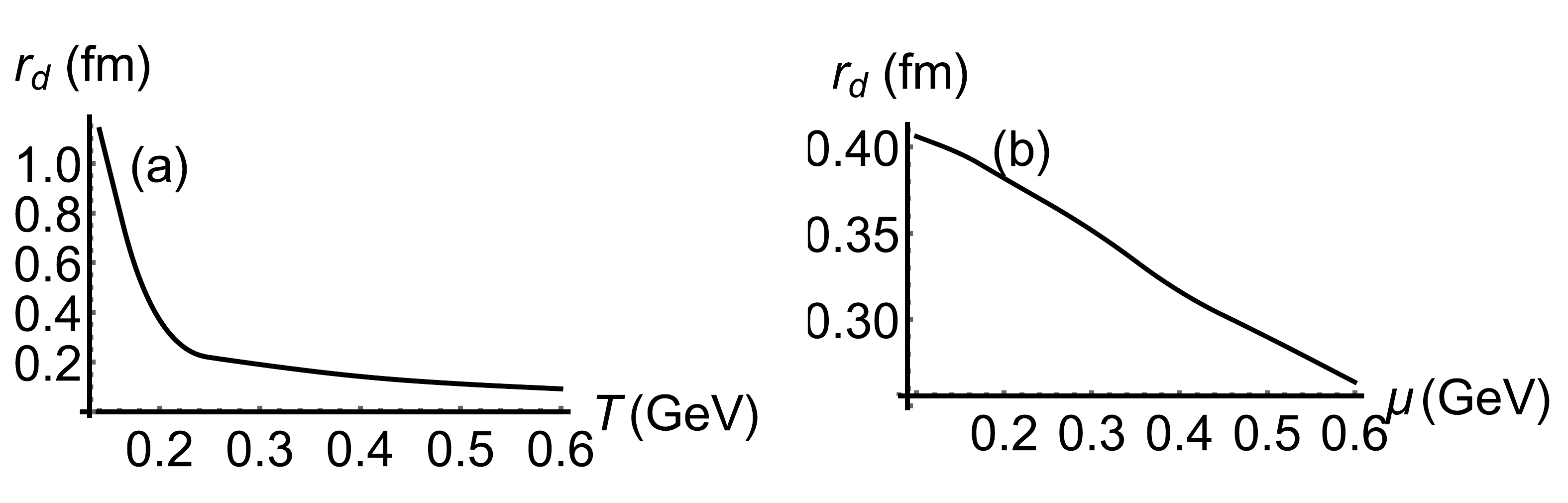
Figure 7. (a) Screening distance
$r_{d}$ as a function of temperature T at μ = 0. (b) Screening distance$r_{d}$ as a function of chemical potential μ at T = 0.2 GeV.Finally, the melting diagram of quark-antiquark pair and triply heavy baryon are shown in Fig. 8. The melting temperature and chemical potential of the quark-antiquark pair are close to those of the triply heavy baryon. Even so, the three lines in Fig. 8 are not totally overlapped. Thus, we again infer that the quark-antiquark pair should be more stable than the triply heavy baryon.
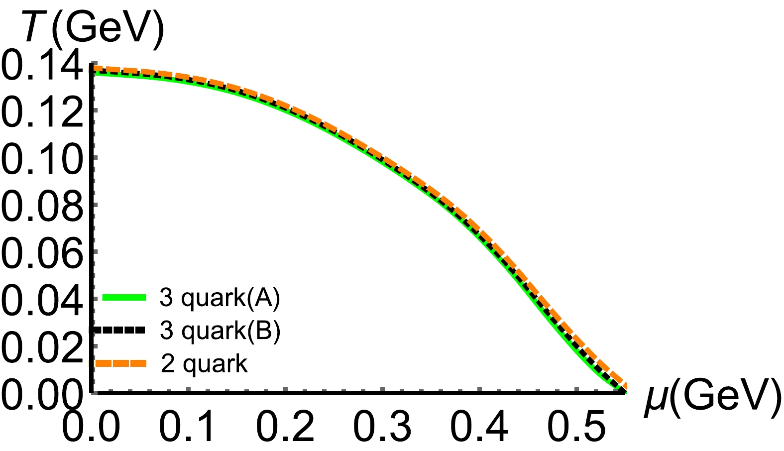
Figure 8. (color online) Three-quark and two-quark melting diagram in the
$T-\mu$ plane. -
We study the potential energy of the triply heavy baryon at finite temperature and chemical potential in this paper. First, the calculation of three-quark potential is presented. With these in hand, numerical results are obtained in the next part. At the vanishing temperature, we fit the lattice results of potential energy and then calculate the separation distance of quarks at finite temperature and chemical potential. The potential energy of triply heavy baryon is shown in the confined and deconfined phases. From the figures of potential energy, we can determine the screening distance. It is found that the screening distance of the quark-antiquark pair is larger than that of the triply heavy baryon at the same temperature and chemical potential. Finally, the melting diagram of the heavy quark-antiquark pair and triply heavy baryon are shown. Although the three lines in the melting diagram are close, we can see the triply heavy baryon is easier to dissolve than the quark-antiquark pair. Moreover, involving the light quarks is an interesting topic. We can continue to discuss the string breaking of QQQ at finite temperature and chemical potential. In the presence of light quarks, we can investigate the string breaking of QQQ. The possible decay channels include
$QQQ \rightarrow QQq + Q\bar q$ ,$QQQ \rightarrow Qqq+ 2Q \bar q$ and$QQQ \rightarrow qqq + 3Q \bar q$ . We will give detailed discussions for future work.
Three-quark potential at finite temperature and chemical potential
- Received Date: 2022-07-20
- Available Online: 2023-01-15
Abstract: Using gauge/gravity duality, we study the potential energy and the melting of triply heavy baryon at finite temperature and chemical potential in this paper. First, we calculate the three-quark potential and compare the results with quark-antiquark potential. With the increase of temperature and chemical potential, the potential energy will decrease at large distances. It is found that the three-quark potential will have an endpoint at high temperature and/or large chemical potential, which means triply heavy baryons will melt at enough high temperature and/or large chemical potential. We also discuss screening distance which can be extracted from the three-quark potential. At last, we draw the melting diagram of triply heavy baryons in the


 DownLoad: