


 Abstract
 HTML
HTML Reference
 Related
 PDF
PDF


-
The AdS/CFT correspondence is known as an essential duality between quantum field theory (QFT) and gravity that corresponds to the classical dynamics of gravity in a higher dimension. The duality was first introduced to connect four dimensional conformal field theory (CFT) to Anti-de Sitter space (AdS) in five dimensions [1–3]. The AdS/CFT correspondence has been applied to a wide range of topics in the physical sciences, such as strong-coupling dynamics (QCD), the physics of black holes and quantum gravity, electroweak theories, and relativistic hydrodynamics [4–33].
One of the most significant challenges in theoretical particle physics is finding an effective field theory (EFT) compatible with quantum gravity. Such theories are situated in the landscape, whereas other incompatible EFTs live in swampland. A universal test to distinguish between these two classes of theories is weak gravity conjecture (WGC). This means that gravity is always the weakest force and reveals an extremality state of the black hole [34–74].
In this paper, we attempt to prove WGC from CFT by studying two critical classes of black holes: hyperscaling violating (HSV) and Kerr-Newman-AdS (KNA) black holes. Because WGC is more consistent at critical points, we use CFT calculations to obtain the critical points associated with the black holes under consideration. Therefore, the remainder of the paper is organized as follows: In Section II, we briefly explain how WGC could be related to CFT. In Section III, we investigate the relationship between WGC and CFT in HSV black holes. We perform a similar analysis for KNA black holes in Section IV. Conclusions and remarks are presented in Section V.
-
Swampland suffers from a lack of global symmetry and completeness of the charge spectrum. Consequently, it cannot present an acceptable explanation for phenomena unless we restrict the global symmetry and there is an upper bound on the mass of several charged conditions [75–79]. Swampland can restrain a complete theory but not EFTs with low energy. Phenomenologically, it is important to understand whether all charged particles are heavy and sufficient regarding black holes or if there are several concepts for the spectrum completeness that prevails at low energies. Swampland conjectures can be used to discuss important issues, for example, they may reveal how close we are to obtaining the status of recovering global symmetries. One can refresh a global symmetry of
$ U(1) $ by transmitting the gauge coupling to 0, which is not permitted in quantum gravity.Attempting to comprehend how string theory prohibits this issue and what drives the incorrect solution if one tries to accomplish this can supply information about the restrictions that EFT must meet to be compatible with quantum gravity. WGC prohibits this methodology owing to the existence of unique light-charged forms that exclude the definition of EFT. This supplies an upper bound on the mass of charged states. In general, WGC includes magnetic and electric versions, providing a gauge theory coupled to gravity. Therefore, we deal with electrically charged Planck units:
$Q/m\geq\mathcal{Q}/M |_{\rm ext}=\mathcal{O}(1)$ [75–79]. Here, Q is the charge, and M determines the mass in the extremal black hole. Moreover,$ Q=qg $ , where q and g are the quantized charges of the state and gauge coupling, respectively.To have WGC with the existence of charge and mass, a charge/mass greater than that in the extremal black hole must be applied. The most specific topic coordinates with Maxwell's theory, which is coupled to gravity; no massless scalar fields exist. Hence, we can construct solutions of R-N black holes by providing a p-form gauge field in d dimensions. WGC indicates the presence of a (
$ p-1 $ )-brane that can meet$ p(d-p-2)T^{2}/d-2 \leq Q^{2}M_{p}^{d-2} $ [13, 61–69, 77, 79]. Here, we note that the motivation for understanding WGC can be found in the physics of black holes. This conjecture expresses that the entire lattice of authorized gauge charges must be settled by physical conditions in an approach with a gauge coupled to gravity. This is not required in quantum field theory because a charged particle can be decoupled from this theory by transmitting the mass to$ \infty $ . The second issue involves breaking global symmetries. There are fascinating relationships between the lack of global symmetries in quantum gravity and spectrum completeness. A typical method of breaking higher form global symmetries includes charged conditions. However, exclusively, if the entire charged condition spectrum exists, can one break the entire group [36–44, 61–69].In this paper, we want to prove or present the emergence of WGC from CFT equations. Hence, we discuss the mixed Klein-Gordon equation against the background of the black hole as a general perturbation and focus on a charged scalar Φ with charge q and mass m [80]
$ \begin{aligned}[b]& \frac{1}{\sqrt{-g}}\partial_{\mu}(g^{\mu\nu}\sqrt{-g}\partial_{\nu}\Phi)-2{\rm i}q g^{\mu\nu}A_{\mu}\partial_{\nu}\Phi\\&-q^2 g^{\mu\nu}A_{\mu}A_{\nu}\Phi-m^2\Phi=0. \end{aligned} $

(1) By inserting
$\Phi= {\rm e}^{-{\rm i}\omega t} \phi({\boldsymbol{x}})$ , we obtain its scalar function, and ω is related to the energy part. Then, we use CFT to find the two-point correlation function of the scalar operator$ J_k $ . We can also find the correlation function based on the ratio of its sub-coefficients as follows [81, 82]$ \begin{equation} \Upsilon_R^{(k)}(\omega)=<J_k(-\omega)J_k(\omega)>=\frac{B_k(\omega)}{A_k(\omega)}. \end{equation} $

(2) Setting
$ A_k(\omega)=0 $ , we can find the location of the poles in the Green function. In such a case, we have$ \omega=\operatorname{Re}(\omega)+\operatorname{Im}(\omega) $ , which has a real part (normal mode) and imaginary part (quasi-normal mode). The imaginary part, which is negative, introduces the inverse relaxation time$ \tau_d $ of the desired mode as$\omega = \operatorname{Re}[\omega] + {\rm i}\operatorname{Im}[\omega] \equiv \operatorname{Re}[\omega] - {\rm i}2\pi / \tau_d$ . Moreover, it describes exponential damping with a characteristic time scale set by$ \tau_d $ .On the other hand, quasi-normal modes play the role of controller for the black hole ringdown to decay or collapse perturbed black holes towards their hairless cases or induce relaxation toward thermal equilibrium after a perturbation period. In addition, quasi-normal modes with the smallest value of
$ \operatorname{Im}[\omega] $ have a less damped state and supervise the thermalization time- scale. Because the black hole ringdown is dual to the thermalization process of CFT [83], the quasi-normal modes appear as the poles of the Fourier transform of the retarded Green function in the context of Ruelle resonances [84].In the context of WGC, we encounter
$ \tau_d>0 $ because the negative values of$ \tau_d $ correspond to an exponentially-growing unstable fundamental state, which threatens the stability of the geometry of black holes. Besides the positive value, it should have a specific bound because the thermalization process cannot occur arbitrarily fast. Hence, we engage a conjecture [81]$ \begin{equation} \tau_d\geq \frac{1}{T}, \end{equation} $

(3) further discussions on which can be found in Refs. [83, 85–90]. Perturbations from different thermalization time scales decay extremely rapidly to satisfy the condition
$ \tau_d >c/T $ . By removing the perturbations from the metric background, it may be found that for a near-extremal charged black hole, there must be at least one particle fulfilling the thermalization rate$ \tau_d > c/T $ .In fact, considering a particle near a black hole leads to the production of perturbations that may be described by the Klein-Gordon equation (1) as the equation of motion of the particle. By solving this equation, we find an imaginary value of energy for the particle, which is connected to Eq. (3). However, the existence of such perturbations makes the black holes unstable so that they approach the extremal limit and consequently connect to the WGC condition. Using the above relationship between Eq. (3) and WGC and also the polarity quantity w obtained during our calculations, we can study the WGC condition from the universal equation (3) (see Refs. [81, 86, 91]).
In the next section, we use the above description for two black holes: HSV and KNA black holes.
-
The metric of a HSV black hole with mass M and charge Q is given by [81, 83, 85, 92]
$ \begin{equation} {\rm d}s^2=r^{\frac{-2\theta}{d}}\left[-r^{2 {z}}f(r){\rm d}t^2+\frac{ {\rm d}r^2}{r^2f(r)}+ r^2 {\rm d}\Omega^2_{k, d}\right], \end{equation} $

(4) where z and θ are dynamical and hyperscaling violation parameters, respectively. Moreover,
$ f(r) $ takes the form$ \begin{equation} f(r)=1+\frac{k}{r^2}\frac{( {d}-1)^2}{( {z}+ {d}-\theta-2)^2}-\frac{M}{r^{ {z}+ {d}-\theta}}+ \frac{Q^2}{r^{2( {z}+ {d}-\theta)}}. \end{equation} $

(5) Here,
$ k=-1, 0, 1 $ determines the hyperboloid, planar, and spherical topologies for the black hole horizon [92]. In this study, we consider$ k=0 $ ; hence, we have$ \begin{aligned}[b] {\rm d}s^2=&r^{\frac{-2\theta}{d}}\left[-r^{2 z}f(r){\rm d}t^2+\frac{ {\rm d}r^2}{r^2f(r)}+ r^2 {\rm d} {\boldsymbol{x}}^2\right], \\ f(r)=&1-\frac{M}{r^{z+d-\theta}}+\frac{Q^2}{r^{2( z+d-\theta)}}, \end{aligned} $

(6) where
${\rm d} {\boldsymbol{x}}^2=\sum_{i=1}^{d}{\rm d}x_i^2$ , and$ x_i $ are spatial coordinates of a d dimensional space. By setting$ f(r_H) = 0 $ , we obtain the event horizon radius$ r_H $ for a charged black hole solution,$ \begin{equation} r_H^{2( {d}+ {z}-\theta-1)}-M r_H^{ {d}+ {z}-\theta-2}+Q^2=0. \end{equation} $

(7) Using the formula
$ T=\dfrac{r_H^{z+1}}{4\pi}|\acute{f}(r_H)| $ and Eq. (6), we can obtain the Hawking temperature [93, 94]$ \begin{equation} T=\frac{( {z}+ {d}-\theta)r_H^{z}}{4\pi}\left(1-\frac{( {z}+ {d}-\theta-2)Q^2}{ {z}+ {d}-\theta} r_H^{2(- {z}- {d}+\theta+1)}\right). \end{equation} $

(8) Therefore, by setting
$ T=0 $ , the extremality bound is obtained by$ \begin{equation} r_H^{2( {z}+ {d}-\theta-1)}=\frac{( {z}+ {d}-\theta-2)}{ {z}+ {d}-\theta} Q^2. \end{equation} $

(9) In this case, we use relations (7) and (9) and rewrite
$ f(r) $ in terms of$ r_H $ $ \begin{aligned}[b] f(r)=&1-\frac{2( {z}+ {d}-\theta-1)}{ {z}+ {d}-\theta-2}\left(\frac{r_H}{r}\right)^{ {z}+ {d}-\theta}\\&+ \frac{ {z}+ {d}-\theta}{ {z}+ {d}-\theta-2}\left(\frac{r_H}{r}\right)^{2( {z}+ {d}-\theta-1)}. \end{aligned} $

(10) Furthermore, the potential is given by [92]
$ \begin{equation} A_t=\frac{\sqrt{2({z}+{d}-\theta)(d-\theta)}}{{z}+ {d}-\theta-2} r_H^{{z}+{d}-\theta-1}\left(\frac{1}{r^{{z}+ {d}-\theta-2}}-\frac{1} {r_H^{{z}+{d}- \theta-2}}\right). \end{equation} $

(11) By changing the corresponding coordinates and examining r near the event horizon, we can write the geometry of
$ AdS_2\times R^{d-1} $ [93] as$ \begin{aligned}[b] r=r_H+\frac{\epsilon r_H^2}{({z}+{d}-\theta)({z}+ {d}-\theta-1)\zeta}, \;\; t=\frac{\tau}{\epsilon r_H^{z}}. \end{aligned} $

(12) Here, note that Eqs. (12), (10), and (6) are obtained with the limit
$ \epsilon \rightarrow 0 $ as follows$ \begin{equation} {\rm d}s^2=r_H^{2-\frac{2\theta}{ {d}}}\left[\frac{-{\rm d}\tau^2+{\rm d}\zeta^2}{( {z}+ {d}-\theta)( {z}+ {d} -\theta-1)\zeta^2}+{\rm d} {\boldsymbol{x}}^2\right]. \end{equation} $

(13) Also, we have
$ \begin{equation} \begin{split} A_\tau=\frac{\sqrt{2( {z}+ {d}-\theta)( {d}-\theta)}}{( {z}+ {d}-\theta)( {z}+ {d}-\theta-1)\zeta}\times r_H^{- {z}+2} \end{split}. \end{equation} $

(14) Now, using Eqs. (1), (13), and (14) with respect to the fact that the metric allows for the separation of variables,
$\Phi(\tau,\zeta, {\boldsymbol{x}})={\rm e}^{-{\rm i}\omega \tau}{\rm e}^{{\rm i} {\boldsymbol{k}}. {\boldsymbol{x}}} \phi(\zeta)$ , we can calculate$ \begin{aligned}[b] & \partial_{\zeta}^2\phi(\zeta)+\left(\omega+\frac{qr_H^{-z+ \rm{2}}\sqrt{2( {z}+ {d}-\theta)( {d}-\theta)} }{( {z}+ {d}-\theta)( {z}+ {d}-\theta-1)\zeta}\right)^2\phi(\zeta)\\&-\frac{k^2+m^2 r_H^{2(1-\frac{\theta}{d})}}{( {z}+ {d}-\theta)( {z}+ {d}-\theta-1)\zeta^2}\phi(\zeta)=0. \end{aligned} $

(15) According to the above equation,
$ -k^2 $ is the eigenvalue of the Laplacian in the flat base sub-manifold. Regarding the above equations,$ \phi(\zeta) $ is obtained in terms of the Whittaker functions, which are given by$ \begin{aligned}[b]\\[-8pt] \phi(\zeta)=&c_1 ~{\rm Whittaker}~ M\left[\frac{-{\rm i}qr_H^{- {z}+2}\sqrt{2( {z}+ {d}-\theta)(d-\theta)} }{( {z}+ {d}-\theta)( {z}+ {d}-\theta-1)},\nu_k,2{\rm i}r\omega\right]\\&+c_2 ~{\rm Whittaker}~ W\left[\frac{-{\rm i}q r_H^{- {z}+2}\sqrt{2( {z}+ {d}-\theta)( {d}-\theta)}}{( {z}+ {d}-\theta)( {z}+ {d}-\theta-1)},\nu_k,2{\rm i}r\omega\right]. \\ \end{aligned} $

(16) Moreover, with respect to the above equation,
$ \nu_k $ is defined by$ \begin{eqnarray} &\nu_k=\sqrt{\frac{1}{4}+\frac{k^2}{( {z}+ {d}-\theta)( {z}+ {d}-\theta-1)}-\frac{q^2 r_H^{- \rm{2z}+4} 2( {z}+ {d}-\theta)( {d}-\theta) }{( {z}+ {d}-\theta)^2( {z}+ {d}-\theta-1)^2}+m^2 r_H^{2(1-\frac{\theta}{ {d}})}}. \end{eqnarray} $

(17) To examine the obtained function
$ \phi(\zeta) $ near the event horizon, we use the limit$ \zeta \longrightarrow 0 $ . Given the properties of the Whittaker function and the definition$ \Delta_k=\frac{1}{2}-\nu_k $ , we have$ \begin{aligned}[b] \phi(\zeta)_{\zeta \rightarrow 0}\approx & C \left[\frac{\Gamma(2\nu_k)(-2{\rm i}\omega)^{\frac{1}{2}-\nu_k}}{\Gamma\Bigg(\dfrac{1}{2}+\nu_k-\dfrac{{\rm i}q r_H^{- {z}+2} \sqrt{2( {z}+ {d}-\theta)( {d}-\theta)}}{( {z}+ {d}-\theta)( {z}+ {d}-\theta-1)}\Bigg)}\zeta^{{\frac{1}{2}-\nu_k}}\right.\\&\left.+\frac{\Gamma(-2\nu_k)(-2{\rm i}\omega)^{\frac{1}{2}+\nu_k}}{\Gamma\left(\dfrac{1}{2}-\nu_k-\dfrac{{\rm i}q r_H^{- {z}+2}\sqrt{2( {z}+ {d}-\theta)( {d}-\theta)} }{( {z}+ {d}-\theta)( {z}+ {d}-\theta-1)}\right)}\zeta^{{\frac{1}{2}+\nu_k}}\right]\\ \equiv &B_k(\omega)\zeta^{\Delta_k}+A_k(\omega)\zeta^{1-\Delta_k}. \end{aligned} $

(18) Using Eqs. (2) and (18), the correlation function is obtained with following equation:
$ \begin{aligned}[b] \mathcal{X}=&\Gamma\big(2\nu_k\big)\Gamma\left(\frac{1}{2}-\nu_k-\frac{{\rm i}q r_H^{- {z}+2} \sqrt{2( {z}+ {d}-\theta)( {d}-\theta)} }{( {z}+ {d}-\theta)( {z}+ {d}-\theta-1)}\right),\\ \mathcal{Y}=&\Gamma\big(-2\nu_k\big)\Gamma\left(\frac{1}{2}+\nu_k-\frac{{\rm i}q r_H^{- {z}+2}\sqrt{2( {z}+ {d}-\theta)( {d}-\theta)} }{( {z}+ {d}-\theta)( {z}+ {d}-\theta-1)}\right),\\ \Upsilon_R^{(k)}(\omega)=&(2\omega)^{-2\nu_k}{\rm e}^{{\rm i}\pi\nu_k}\times\frac{\mathcal{X}}{\mathcal{Y}}. \end{aligned} $

(19) According to Eq. (19), there is no ω with an imaginary part; as a result, WGC can not be discussed. Now, we consider the condition
$ r_H \rightarrow r_H+\dfrac{\epsilon r_H^2}{({z}+ {d}-\theta)({z}+ {d}-\theta-1)\zeta_0} $ with respect to Eqs. (13) and (14) and hence obtain$ \begin{aligned}[b] {\rm d}s^2=&\frac{r_H^{2-\frac{2\theta}{ {d}}}}{( {z}+ {d}-\theta)( {z}+ {d}-\theta-1)\zeta^2}\\&\times\left[-\left(1-\frac{\zeta^2}{\zeta_0^2}\right){\rm d}\tau^2+ \left(1-\frac{\zeta^2}{\zeta_0^2}\right)^{-1}{\rm d}\zeta^2\right] +r_H^{2-\frac{2\theta}{ {d}}}{\rm d} {\boldsymbol{x}}^2, \end{aligned} $

(20) and
$ \begin{equation} A_\tau=\frac{\sqrt{2( {z}+ {d}-\theta)( {d}-\theta)}}{( {z}+ {d}-\theta)( {z}+ {d}-\theta-1)\zeta} r_H^{- {z}+2}\left(1-\frac{\zeta}{\zeta_0}\right). \end{equation} $

(21) The temperature associated with the metric in Eq. (20) is
$ T = 1/2\pi \zeta_0 $ . Using Eqs. (1), (20), and (21) with respect to the fact that the metric allows for the separation of variables,$\Phi(\tau,\zeta, {\boldsymbol{x}})={\rm e}^{-{\rm i}\omega \tau}{\rm e}^{{\rm i} {\boldsymbol{k}}. {\boldsymbol{x}}} \phi(\zeta)$ , we can calculate$ \begin{aligned}[b] &\partial_{\zeta}^2\phi(\zeta)+\frac{2\zeta}{\zeta^2-\zeta_0^2}\partial_{\zeta}\phi(\zeta)\\&+ \frac{\left[\omega+\dfrac{q r_H^{- {z}+2} \sqrt{2( {z}+ {d}-\theta)( {d}-\theta)} \left(1-\dfrac{\zeta}{\zeta_0}\right)}{( {z}+ {d}-\theta)( {z}+ {d}-\theta-1)\zeta}\right]^2}{\left(1-\dfrac{\zeta^2}{\zeta_0^2}\right)^2}\phi(\zeta)\\ &-\frac{k^2+m^2 r_H^{2(1-\frac{\theta}{ {d}})}}{( {z}+ {d}-\theta)( {z}+ {d}-\theta-1)\zeta^2\left(1-\dfrac{\zeta^2}{\zeta_0^2}\right)}\phi(\zeta)=0. \end{aligned} $

(22) By solving the above equation,
$ \phi(\zeta,\omega) $ is obtained using$ \begin{aligned}[b] &\phi_k(\zeta,\omega)\sim \left(\frac{1}{\zeta}-\frac{1}{\zeta_0}\right)^{-\frac{1}{2}\mp\nu_k}\left(\frac{\zeta_0+\zeta}{\zeta_0-\zeta}\right)^{{\rm i}\omega \zeta_0-{\rm i}\frac{q r_H^{- {z}+2} \sqrt{2( {z}+ {d}-\theta)( {d}-\theta)}}{( \rm{z+d}-\theta)( \rm{z+d}-\theta-1)}} F_1\bigg\{\frac{1}{2}\pm \nu_k+{\rm i}\omega \zeta_0-{\rm i}\frac{q \sqrt{2( {z}+ {d}-\theta)( {d}-\theta)} r_H^{- {z}+2}}{( {z}+ {d}-\theta)( {z}+ {d}-\theta-1)}, \frac{1}{2}\pm \nu_k\\ &+-{\rm i}\frac{q \sqrt{2( {z}+ {d}-\theta)( {d}-\theta)} r_H^{- {z}+2}}{( {z}+ {d}-\theta)( {z}+ {d}-\theta-1)},\frac{1}{2}\pm \nu_k,\frac{2\zeta}{\zeta-\zeta_0}\bigg\}. \\ \end{aligned} $

(23) We examine the above solution on the AdS boundary. In this case, using the properties of the hypergeometric functions and Eq. (2), we obtain the retarded Green function as follows:
$ \begin{aligned}[b] \mathcal{A}=&\Gamma\big(1+2\nu_k\big)\Gamma\bigg(\frac{1}{2}-\nu_k-\frac{{\rm i}\omega}{2\pi T}+\frac{{\rm i}q r_H^{- {z}+2}\sqrt{2( {z}+ {d}-\theta)( {d}-\theta)}}{( {z}+ {d}-\theta)( {z}+ {d}-\theta-1)}\bigg) \Gamma\bigg(\frac{1}{2}-\nu_k+\frac{{\rm i}qr_H^{- {z}+2}\sqrt{2( {z}+ {d}-\theta)( {d}-\theta)}}{( {z}+ {d}-\theta) ( {z}+ {d}-\theta-1)}\bigg),\\ \mathcal{B}=&\Gamma\big(1-2\nu_k\big)\Gamma\bigg(\frac{1}{2}+\nu_k-{\rm i}\frac{\omega}{2\pi T}+\frac{{\rm i}q r_H^{- {z}+2}\sqrt{2( {z}+ {d}-\theta)( {d}-\theta)}}{( {z}+ {d}-\theta)( {z}+ {d}-\theta-1)}\bigg) \Gamma\bigg(\frac{1}{2}+\nu_k+\frac{{\rm i}qr_H^{- {z}+2}\sqrt{2( {z}+ {d}-\theta)( {d}-\theta)}}{( {z}+ {d}-\theta) ( {z}+ {d}-\theta-1)}\bigg),\\ \Upsilon_R^{(k)}(\omega)=&(4\pi T)^{-2\nu_k}\times\frac{\mathcal{A}}{\mathcal{B}}. \end{aligned} $

(24) Here, we use the explicit definition of T instead of
$ \zeta_0 $ . When we obtain the polarity of Eq. (2), ω has two parts, real and imaginary, as$\omega={\rm Re}(\omega)+{\rm Im}(\omega)$ .$ \begin{equation} \omega=\frac{q r_H^{- {z}+2}\sqrt{2( {z}+ {d}-\theta)( {d}-\theta)}}{( {z}+ {d}-\theta)( {z}+ {d}-\theta-1)}-{\rm i}2\pi T\left(\frac{1}{2}+n+\nu_k\right). \end{equation} $

(25) Here, we can discuss WGC because we have a quasi-normal mode. Hence, note here that we are interested in the system's response at low frequencies [83, 86, 91].
$ \begin{aligned}[b] \tau_d \equiv & \tau_d^{(0,0)}= \frac{1}{T(\frac{1}{2}+\nu_0)}, \\ \nu_0=&\sqrt{\frac{1}{4}-\frac{2q^2 r_H^{-2 {z}+4}( {z}+ {d}-\theta)( {d}-\theta)}{( {z}+ {d}-\theta)^2( {z}+ {d}-\theta-1)^2}+m^2 r_H^{2(1-\frac{\theta}{ {d}})}}. \end{aligned} $

(26) Now, using Eqs. (3) and (26), we obtain the following condition:
$ \begin{aligned}[b]& \left(m r_H^{1-\frac{\theta}{ {d}}}-\frac{q r_H^{- {z}+2} \sqrt{2( {z}+ {d}-\theta)( {d}-\theta)}}{( {z}+ {d}-\theta)( {z}+ {d}-\theta-1)}\right)\\&\times\left(m r_H^{1-\frac{\theta}{ {d}}}+\frac{q r_H^{- {z}+2} \sqrt{2( {z}+ {d}-\theta)( {d}-\theta)}}{( {z}+ {d}-\theta)( {z}+ {d}-\theta-1)}\right)<0. \end{aligned} $

(27) The WGC condition is satisfied when we have the following expression
$ \begin{equation} r_H^{1-\frac{\theta}{ {d}}}=\frac{ r_H^{- {z}+2} \sqrt{2( {z}+ {d}-\theta)( {d}-\theta)}}{( {z}+ {d}-\theta)( {z}+ {d}-\theta-1)}. \end{equation} $

(28) According to Eq. (27), we can rewrite the radius of the event horizon in terms of dynamic parameters as follows:
$ \begin{equation} r_H^{z-\frac{\theta}{d}-1}=\frac{ \sqrt{2(z+d-\theta)(d-\theta)}}{(z+d-\theta)(z+d-\theta-1)}. \end{equation} $

(29) This relation shows the compatibility of WGC and CFT only on the horizon of a specific event obtained from Eq. (29). According to the relation in Eq. (9), r is positive when
$ {z}+ {d}-\theta>2 $ . The solution to the above relationship is when$ {z}=1, {d}=1 $ , and$ \theta\rightarrow 0^- $ or$ {z} \rightarrow1^+, {d}=1 $ , and$ \theta =0 $ .To drive WGC from the CFT viewpoint, we must specify a series of specific points and discuss the compatibility of these two structures at these points. Because
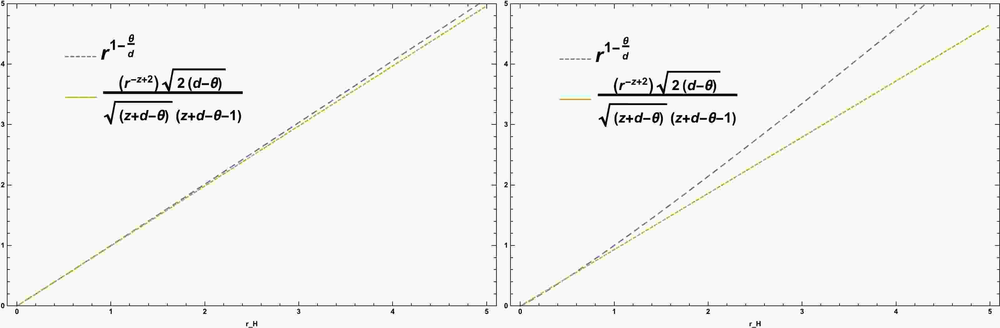
$ r_H $ represents the position of the entire horizon, we cannot discuss the relation between the WGC of CFT for the parameters of the entire horizon. Therefore, we must inevitably determine a specific value for$ r_{H} $ by setting several important parameters, such as z, d, and θ, to find specific points of$ r_H $ . Consequently, by setting$ r_H<1 $ and for a series of specific points, WGC and CFT are aligned. As shown in Fig. 1, when θ is closer to zero, WGC holds for larger values of$ r_H $ . In this case, it is set for both$ r_H $ greater and less than one. As shown in Fig. 2, when$ {z} $ is closer to one,$ r_H $ can be established for different values; however, when$ {z} $ is slightly larger than one, WGC for$ r_H<1 $ will be established. When$ \theta< {d} $ , we have a solution for a value of$ r_H<1 $ . As shown in Fig. 3, when we consider θ to be a number less than zero and z and d to be greater than one, WGC will hold for$r_H < 1 $ .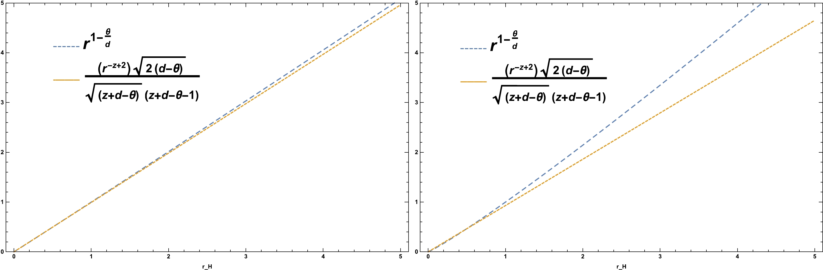
Figure 1. (color online) Left plot:
$ z=1 $ ,$ d = 1 $ , and$ \theta = -0.01 $ . Right plot:$ z=1 $ ,$ d = 1 $ , and$ \theta = -0.1 $ .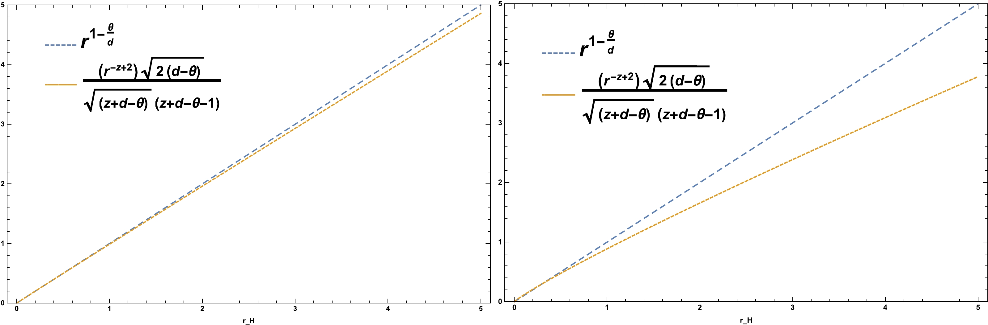
Figure 2. (color online) Left plot:
$ z=1.01 $ ,$ d = 1 $ , and$ \theta = 0 $ . Right plot:$ z=1.1 $ ,$ d = 1 $ , and$ \theta = 0 $ .
Figure 3. (color online) Left plot:
$ z=1.5 $ ,$ d = 2 $ , and$ \theta = -1 $ . Right plot:$ z=2 $ ,$ d = 3 $ , and$ \theta = -2 $ . -
Analogous to the previous type of black hole, we attempt to obtain the wave function and energy spectrum of KNA black holes. Here, we find that our black hole is unstable, which is proof of WGC. To observe such a condition for the corresponding black hole, we consider the Boyer-Lindquist-type coordinates [94],
$ \begin{aligned}[b] {\rm d}s^2=&-\frac{f(r)}{\rho^2}\left({\rm d}t-\frac{a \sin^2\theta}{\Xi}{\rm d}\phi\right)^2+\frac{\rho^2}{f(r)}{\rm d}r^2+\frac{\rho^2}{f(\theta)}{\rm d}\theta^2 \\&+\frac{f(\theta)}{\rho^2}\sin^2\theta\left(a{\rm d}t-\frac{(r^2+a^2)}{\Xi}{\rm d}\phi\right)^2, \end{aligned} $

(30) where
$ \begin{aligned}[b]& f(r)={(r^2+a^2)\left(1+\frac{r^2}{\ell^2}\right)-2Mr+Q^2} , \\& f(\theta)={1-\frac{a^2}{\ell^2}\cos^2\theta}, \\& \rho^2={r^2+a^2 \cos^2\theta}, \\& \Xi={1-\frac{a^2}{\ell^2}}. \end{aligned} $

(31) Here, a is a rotational parameter, and Q is the electric charge.
$ \ell^2 $ is related to the cosmological constant; when it is positive, we have$dS$ , and when it is negative, we have$ AdS $ . Its vector potential is considered as follows$ \begin{equation} A=-\frac{Qr}{\rho^2}\left({\rm d}t-\frac{a \sin^2 \theta}{\Xi}{\rm d}\phi \right). \end{equation} $

(32) The Hawking temperature, entropy, and angular velocity of the horizon are obtained using
$ \begin{aligned}[b] {T_H}=&{\frac{r_+ \left(1+\dfrac{a^2}{\ell^2}+\dfrac{3 r_+^2}{\ell^2}-\dfrac{a^2+Q^2}{r_+^2}\right)}{4 \pi (r_+^2+a^2)}} , \\ S=&{\frac{\pi(r_+^2+a^2)}{\Xi}},\\ {\Omega_H}=&{\frac{a\Xi}{r_+^2+a^2}}. \end{aligned} $

(33) We can rewrite
$ f(r) $ near the event horizon in the quadratic order as follows [95]:$ \begin{equation} f(r)\simeq k(r-r_+)(r-r_*), \quad k=1+\frac{a^2}{\ell^2}+\frac{6r_+^2}{\ell^2}, \end{equation} $

(34) where
$ r_+ $ is the radius of the external event horizon, and$ r_* $ is the radius of another horizon. In the extremality limit, the following conditions also apply [95]$ r_+^2\geq\frac{\ell^2}{6}\left(\sqrt{\left(1+\frac{a^2}{\ell^2}\right)^2+12\frac{a^2}{\ell^2}}-\left(1+\frac{a^2}{\ell^2}\right)\right). $

(35) In the limit
$ \dfrac{a}{\ell}\ll 1 $ , we can consider the minimum value of$ r_+ $ equal to a. By setting$ f(r)=0 $ and$ T_H=0 $ , we can obtain the extreme state of the black hole with the condition$ r_+=a $ as follows$ \begin{equation} k=\frac{M_{exe}}{r_+}+\frac{4r_+^2}{\ell^2}. \end{equation} $

(36) We now use Eq. (1) to solve Klein Gordon's equation in the background of the KNA black hole and obtain the correlation function, which is calculated using the following equation [95]
$ \begin{aligned}[b] \Upsilon_R=&\frac{\Gamma(1-2h_Q)}{\Gamma(2h_Q-1)}\\&\times\frac{\Gamma\left(h_Q+{\rm i}\dfrac{\omega_L-Q_L \mu_L}{2\pi T_L}\right)\Gamma\left(h_Q+{\rm i}\dfrac{\omega_R-Q_R \mu_R}{2\pi T_R}\right)}{\Gamma\left(1-h_Q+{\rm i}\dfrac{\omega_L-Q_L \mu_L}{2\pi T_L}\right)\Gamma\left(1-h_Q+{\rm i}\dfrac{\omega_R-Q_R \mu_R}{2\pi T_R}\right)}, \end{aligned} $

(37) where
$ \begin{aligned}[b] {\omega_L}=&{\frac{r_+^2+r_*^2+2a^2}{2 a \Xi}\omega}, \quad {\omega_R}={\frac{r_+^2+r_*^2+2a^2}{2 a \Xi}\omega-M},\\ {Q_L}=&Q_R={e} \\ {\mu_L}=&{\frac{Q(r_+^2+r_*^2+2a^2)}{2 a \Xi (r_+ + r_*)}}, \quad {\mu_R}={\frac{Q(r_+ + r_*)}{2 a \Xi}},\\ {T_L}=&{\frac{k(r_+^2+r_*^2+2a^2)}{4\pi a \Xi (r_+ + r_*)}}, \quad {T_R}={\frac{k(r_+ - r_*)}{4\pi a \Xi}}, \end{aligned} $

(38) and we also have
$ \begin{equation} h_Q=\frac{1}{2}+\frac{1}{2}\sqrt{1-4\left(\frac{e^2 Q^2}{k^2}-\frac{K_Q}{k}\right)}, \end{equation} $

(39) where
$ K_Q $ is the separation constant [95]. The pole of Eq. (37) is given as follows:$ \begin{equation} 1-h_Q+{\rm i}\frac{\omega_L-Q_L \mu_L}{2\pi T_L}=-n, \quad 1-h_Q+{\rm i}\frac{\omega_R-Q_R \mu_R}{2\pi T_R}=-n. \end{equation} $

(40) Because the above two relations are similar, we consider only one of them and place it in Eq. (3) with the condition
$ K_Q=-3k $ to obtain the following equation:$ \begin{equation} \frac{e Q}{k}>1. \end{equation} $

(41) Using Eqs. (35), (36), and (41) along with the condition
$ \dfrac{a}{\ell}\ll 1 $ , we obtain$ \begin{equation} \frac{e a Q}{M_{exe}+\dfrac{4a^3}{\ell^2}}>1. \end{equation} $

(42) The above statement satisfies the WGC condition for
$ \dfrac{a}{\ell}\ll 1 $ and$ e=\dfrac{1}{a} $ .The initial arguments on WGC are presented for the physics of black holes, followed by several expansions in different parts.
The primary characteristics of black holes are addressed through the laws of thermodynamics and its relation with gravity based on the AdS/CFT correspondence. In this study, we show that WGC is related to the thermalization dynamics governing the relaxation process after a perturbation process. The validity of such a result is guaranteed by having a lower bound on the thermalization time scale. In fact, CFT gives a lower thermalization bound on the thermalization time-scale to charged-near-extremal black holes, which can be used as a necessary condition to reach the definition of WGC. Using the model's free parameters, we determine a series of parametric points and regions and then check WGC at these points. Note that imposing more restrictions might allow one to determine the exact range of compatibility between WGC and CFT. After considering common points originating from gravity, thermodynamics, and the relationship between gravity and WGC, the thermodynamics of black holes can be chosen to enter WGC and challenge different theories for a better understanding of the link between gauge theories and quantum gravity.
-
The idea of WGC has been applied in many cosmological structures, such as inflation, dark energy, and black holes physics. On the other hand, CFT is widely used the literature of theoretical particle physics, particularly in AdS/CFT correspondence. However, the connection between the two theories navigates us to several interesting results. The main aim of this paper is to study the relationship between WGC and CFT using HSV and KNA black holes. To fulfill this, we use the correlation function of CFT. Hence, we obtain proof for predicting WGC on the CFT side, which indicates the emergence of WGC from correlation function calculations in the considered black holes. Because WGC at critical points offers compatibility results, it also appears in the extremality bound of black holes. Assuming this and the CFT correlation function, we calculate the critical points of the black holes. Hence, WGC appears for both black holes. In addition to proving WGC, we also show the exciting close relationship between WGC and CFT. In this case, we use the correlation function in CFT and its poles. Moreover, we obtain the energy spectrum of the black holes, including two parts, that is, real (normal mode) and imaginary (quasi-normal mode). We find that when
$ z=1 $ ,$ d=1 $ , and$ \theta\rightarrow 0^{-} $ , WGC emerges in HSV black holes because it contains$ r_{H} $ values larger and smaller than one. In other cases, WGC is only valid for$ r_H $ values less than one. The condition of WGC for KNA black holes is related to the rotation and radius parameters if the charged particle near the black hole is$\dfrac{1}{a}$ and has a ratio such as$\dfrac{a}{\ell}\ll 1$ . Because a relationship between these two ideas has somehow emerged, we can perform further calculations to analyze the results and even reach a correspondence between the two theories, which we shall examine in future studies.
Weak gravity conjecture from conformal field theory: a challenge from hyperscaling violating and Kerr-Newman-AdS black holes
- Received Date: 2022-07-15
- Available Online: 2023-01-15
Abstract: We search for a possible relationship between weak gravity conjecture (WGC) and conformal field theory (CFT) in hyperscaling violating and Kerr-Newman-AdS black holes. We deal with the critical points of the black hole systems using the correlation function introduced in CFT and discuss WGC conditions using the imaginary part of the energy obtained from the critical points and their poles. Under the assumptions


 DownLoad: