


 Abstract
 HTML
HTML Reference
 Related
 PDF
PDF


-
Recently, the LHCb collaboration [1] reported the observation of a very narrow state, called
$ T_{cc}^+ $ , in the$ D^0D^0\pi^+ $ invariant mass spectrum. The binding energy and the decay width is:$ \begin{aligned}[b] \delta m_{\rm{BW}}=& -273 \pm 61 \pm 5^{+11}_{-14}\; \rm{keV/c^2}, \\ \Gamma_{\rm{BW}}=&\; 410 \pm 165 \pm 43^{+18}_{-38} \;\rm{keV}. \end{aligned} $

(1) The LHCb collaboration also released a decay analysis, in which the unitarised Breit–Wigner profile was used [2]. The mass with respect to the
$ D^{*+}D^0 $ threshold and width reads,$ \begin{aligned}[b] \delta m^{U}=& -360 \pm 40^{+4}_{-0}\; \rm{keV/c^2}, \\ \Gamma^{U}=& \;48 \pm 2^{+0}_{-14} \;\rm{keV}. \end{aligned} $

(2) This observation has two points worth our attention. Firstly, different from the hidden charm or hidden bottom exotic hadron states previously observed experimentally, this is the first observation of an exotic state with open double charm. Dating back to the year of 2002, the SELEX collaboration first reported the observation of the doubly-charmed baryon
$ \Xi_{cc}^+ (ccd) $ in the channels$ \Lambda_c^+K^-\pi^+ $ and$ pD^+K^- $ [3, 4]. Fifteen years later, the LHCb collaboration also found the doubly-charmed baryon$ \Xi_{cc}^{++}(ccu) $ in the$ \Lambda_c^+K^-\pi^+\pi^+ $ mass distribution [5]. The value of the mass is 100 MeV higher than the$ \Xi_{cc}^+ $ observed by the SELEX collaboration. Secondly, the mass of the observed$ T_{cc} $ is just a litter lower than$ M(D^0)+M(D^{*+}) $ , with a very small binding energy. Undoubtedly, the observation of$ T_{cc}^+ $ will open a brand new window to search for new hadron states beyond the traditional hadrons, both experimentally and theoretically.The discoveries of
$ T_{cc}^+ $ and$ \Xi_{cc}^{++} $ have an important impact, since they indicate that two identical charm quarks can exist in a hadronic state, which inspires some theoretical studies on possible doubly-charmed tetraquarks and their partner states, doubly-bottomed tetraquarks. Historically, the first study of$ QQ\bar{q}\bar{q} $ was made in early 1980s [6], with the observation that the system will be bound, below the$ Q\bar{q}+Q\bar{q} $ threshold, if the mass ratio$ M/m $ becomes large enough. This was confirmed by Heller et al. [7, 8] and Zouzou et al. [9]. The first phenomenological attempt to estimate doubly-heavy tetraquark mass was carried out by Lipkin using the nonrelativistic quark model in 1986 [10]. The author pointed out$ M_{T_{cc}} \leq 3935 $ MeV, 60 MeV above the threshold, and$ T_{bb} $ was a bound state with the binding energy of 224 MeV.Until now, there have been many articles published about the doubly-heavy tetraquarks
$ QQ\bar{q}\bar{q} \ (Q = c, b ; $ $ q = u, d, s) $ , such as the color–magnetic interaction (CMI) model [11–16], quark models [17–35], the QCD sum rule approach [36–46], lattice QCD simulations [47–55], effective field theory [56–58] and others [59–64]. One of the controversies is whether$ QQ\bar{q}\bar{q} $ tetraquarks with two heavy quarks Q and two light antidiquarks$ \bar{q} $ are stable or not against the decay into two$ Q\bar{q} $ mesons. Actually, this dispute has a long history, due to the lack of experimental information about the strength of the interaction between two heavy quarks. The other important question is, if the$ T_{QQ} $ is bound, is it tightly bound or loosely bound?Most theoretical calculations predict that the double-bottom tetraquark states, at least the
$ 1^+ $ states, lie below the open-bottom threshold. Conversely, for doubly-charmed tetraquarks, some works suggest they are above the open-charm threshold [18, 25, 36, 37, 39, 48, 65]. In Ref. [65], the authors stated that$ T_{cc} $ was a$ I(J^P) = 0(1^+) $ state around 3929 MeV (53 MeV above the$ DD^* $ threshold) and all the double-charm tetraquarks were not stable. Karliner et al. [18] predicted the mass of$ T(cc\bar{u}\bar{d}) $ with$ J^P = 1^+ $ to be 3882 MeV, 7 MeV above the$ D^0D^{*+} $ threshold and 148 MeV above the$ D^0D^+\gamma $ threshold against the strong and weak decays. In lattice QCD simulations, the authors [48] showed that the phase shifts in the isospin triplet ($ I = 1 $ ) channels indicated repulsive interactions, while those in the$ I = 0 $ channels suggested attraction, although neither bound states nor resonance states were found in the$ T_{cc} (IJ^P = 01^+) $ . Some works are in favor of them as tightly bound states [11–13, 23, 35]. The common feature of research obtaining a deeply bound state is that the diquark–antidiquark structure is employed. For example, in Ref. [12], the mass splitting indicated that the mass of$ T_{cc} $ with color structure$ 6\otimes\bar{6} $ lay above the$ DD^* $ threshold, but the mass of$ T_{cc} $ with color structure$ \bar{3}\otimes3 $ lay at 71 MeV below the$ DD^* $ threshold. On the other hand, in Ref. [14], Li et al. obtained a loosely-bound molecule state with a 470-keV binding energy, which was consistent with the recent experimental data [1, 2]. In their work, only the meson–meson structure was considered. These theoretical works suggest that color structures and quark–quark interactions may play an important role in the$ T_{QQ} $ states.The discovery of the
$ T_{cc} $ state provides a chance to check the quark–quark interactions for various theoretical approaches based on quark degrees of freedom. In the quark model, quark–quark interactions within the confinement scale (~ 1 fm) have undergone a wide check in the hadron spectrum, where the unique color structure, singlet, is accepted. When we apply quark–quark interactions to multiquark systems, Casimir scaling is employed for generalization [66], although this generalization may cause anti-confinement in multiquark systems [67]. In the Casimir scaling scheme, the two-body interactions used in color singlet$ qqq $ and$ q\bar{q} $ systems are directly extended to quark-pairs with various color structures, and the effects of color structure are taken care of by the Casimir operator$ {\boldsymbol{\lambda}}_i\cdot {\boldsymbol{\lambda}}_j $ .With the accumulation of experimental data on multiquark systems, it is time to check Casimir scaling in detail. Here, we apply the chiral quark model (ChQM) to the tetraquark system
$ T_{QQ} $ with meson–meson and diquark–antidiquark structures, and generalize the quark–quark interactions used in color-singlet baryons and mesons to multiquark systems using Casimir scaling. The contributions of each term in the Hamiltonian for different color structures are extracted, and used to study the effects of color structure. In this way, we are trying to make clear why the diquark–antiquark structure leads to deeply bound states, whereas the meson–meson structure brings about weakly bound states. In the present work, we investigate the doubly-heavy tetraquarks$ cc\bar{u}\bar{d} $ and$ bb\bar{u}\bar{d} $ with the quantum numbers$ I(J^P) = 1(0^+), 1(1^+), 1(2^+), $ $ 0(1^+) $ constrained by the Pauli principle in the framework of the ChQM. Single-channel and various channel-coupling calculations are performed to show the influence of color structure. Meanwhile, the possible resonance states are also searched with a real scaling method [68] in the complete coupled channels.The paper is organized as follows. In the next section, we present the chiral quark model (ChQM) and the accurate few-body computing method—the Gaussian expansion method (GEM) [69]—as well as the wave functions of the four-body
$ T_{QQ} $ system. In Sec. III, we present and analyze our results. Finally, a summary is given in the last section. -
Many theoretical methods have been used to uncover the properties of multiquark candidates observed in experiments since 2003. One of them, the QCD-inspired quark model, is still the most effective and simple tool to describe the hadron spectra and hadron–hadron interactions, and has produced great achievements. It has been used in our previous work to investigate the tetraquark systems and obtain some helpful information [70-72]. Here, the application of the chiral quark model in doubly-heavy tetraquark states
$ T_{QQ} $ is quite expected.The Hamiltonian of the chiral quark model can be written as follows for a four-body system,
$ \begin{aligned}[b] H =& \sum\limits_{i = 1}^4 m_i +\frac{p_{12}^2}{2\mu_{12}}+\frac{p_{34}^2}{2\mu_{34}} +\frac{p_{1234}^2}{2\mu_{1234}} \\ & + \sum\limits_{i<j = 1}^4 \left[ V_{ij}^{C}+V_{ij}^{G}+\sum\limits_{\chi = \pi,K,\eta} V_{ij}^{\chi} +V_{ij}^{\sigma}\right]. \end{aligned} $

(3) The potential energy terms
$ V_{ij}^{C, G, \chi, \sigma} $ represent confinement, one-gluon exchange (OGE), Goldstone boson exchange and scalar σ-meson exchange, respectively. According to the Casimir scheme, the forms of these potentials can be directly extended to multiqaurk systems with the Casimir factor$ {\boldsymbol{\lambda}}_i \cdot {\boldsymbol{\lambda}}_j $ [66]. Their forms are:$ V_{ij}^{C}= ( -a_c r_{ij}^2-\Delta ) {\boldsymbol{\lambda}}_i^c \cdot {\boldsymbol{\lambda}}_j^c , $

(4) $ V_{ij}^{G}= \frac{\alpha_s}{4} {\boldsymbol{\lambda}}_i^c \cdot {\boldsymbol{\lambda}}_{j}^c \left[\frac{1}{r_{ij}}-\frac{2\pi}{3m_im_j}{\boldsymbol{\sigma}}_i\cdot {\boldsymbol{\sigma}}_j \delta({\boldsymbol{r}}_{ij})\right], $

(5) $ \delta{({\boldsymbol{r}}_{ij})} = \frac{{\rm e}^{-r_{ij}/r_0(\mu_{ij})}}{4\pi r_{ij}r_0^2(\mu_{ij})}, $

(6) $ V_{ij}^{\pi}= \frac{g_{ch}^2}{4\pi}\frac{m_{\pi}^2}{12m_im_j} \frac{\Lambda_{\pi}^2}{\Lambda_{\pi}^2-m_{\pi}^2}m_\pi v_{ij}^{\pi} \sum\limits_{a = 1}^3 \lambda_i^a \lambda_j^a, $

(7) $ V_{ij}^{K}= \frac{g_{ch}^2}{4\pi}\frac{m_{K}^2}{12m_im_j} \frac{\Lambda_K^2}{\Lambda_K^2-m_{K}^2}m_K v_{ij}^{K} \sum\limits_{a = 4}^7 \lambda_i^a \lambda_j^a, $

(8) $ \begin{aligned}[b] V_{ij}^{\eta} =& \frac{g_{ch}^2}{4\pi}\frac{m_{\eta}^2}{12m_im_j} \frac{\Lambda_{\eta}^2}{\Lambda_{\eta}^2-m_{\eta}^2}m_{\eta} v_{ij}^{\eta} \\ & \times \left[\lambda_i^8 \lambda_j^8 \cos\theta_P - \lambda_i^0 \lambda_j^0 \sin \theta_P \right],\end{aligned} $

(9) $ v_{ij}^{\chi} = \left[ Y(m_\chi r_{ij})- \frac{\Lambda_{\chi}^3}{m_{\chi}^3}Y(\Lambda_{\chi} r_{ij}) \right] {\boldsymbol{\sigma}}_i \cdot{\boldsymbol{\sigma}}_j, $

(10) $ \begin{aligned}[b] V_{ij}^{\sigma}=& -\frac{g_{ch}^2}{4\pi} \frac{\Lambda_{\sigma}^2}{\Lambda_{\sigma}^2-m_{\sigma}^2}m_\sigma \\ &\times \left[ Y(m_\sigma r_{ij})-\frac{\Lambda_{\sigma}}{m_\sigma}Y(\Lambda_{\sigma} r_{ij})\right] , \end{aligned} $

(11) where
$ Y(x) = {\rm e}^{-x}/x $ ;$ \{m_i\} $ are the constituent masses of quarks and antiquarks, and$ \mu_{ij} $ are their reduced masses;$ \mu_{1234} = \frac{(m_1+m_2)(m_3+m_4)}{m_1+m_2+m_3+m_4}; $

(12) $ {\boldsymbol{p}}_{ij} = ({\boldsymbol{p}}_i-{\boldsymbol{p}}_j)/2 $ ,$ {\boldsymbol{p}}_{1234} = ({\boldsymbol{p}}_{12}-{\boldsymbol{p}}_{34})/2 $ ;$ r_0(\mu_{ij}) = s_0/\mu_{ij} $ ;$ {\boldsymbol{\sigma}} $ are the$ SU(2) $ Pauli matrices;$ {\boldsymbol{\lambda}} $ ,$ {\boldsymbol{\lambda}}^c $ are$ SU(3) $ flavor and color Gell-Mann matrices, respectively;$ g^2_{ch}/4\pi $ is the chiral coupling constant, determined from π-nucleon coupling; and$ \alpha_s $ is an effective scale-dependent running coupling [73],$ \alpha_s(\mu_{ij}) = \frac{\alpha_0}{\ln\left[(\mu_{ij}^2+\mu_0^2)/\Lambda_0^2\right]}. $

(13) All the parameters are determined by fitting the meson spectra, from light to heavy, and the resulting values are listed in Table 1.
Quark masses /MeV $ m_u=m_d $ 

313 $ m_s $ 

536 $ m_c $ 

1728 $ m_b $ 

5112 Goldstone bosons $ m_{\pi} $ 

0.70 (fm $ ^{-1} \sim 200\, $ MeV)

$ m_{\sigma} $ 

3.42 $ m_{\eta} $ 

2.77 $ m_{K} $ 

2.51 $ \Lambda_{\pi}=\Lambda_{\sigma} $ 

4.2 $ \Lambda_{\eta}=\Lambda_{K} $ 

5.2 $ g_{ch}^2/(4\pi) $ 

0.54 $ \theta_p(^\circ) $ 

−15 Confinement $ a_c $ /(MeV fm

$ ^{-2} $ )

101 Δ/MeV −78.3 OGE $ \alpha_0 $ 

3.67 $ \Lambda_0/{\rm fm}^{-1} $ 

0.033 $ \mu_0 $ /MeV

36.98 $ s_0 $ /MeV

28.17 Table 1. Model parameters, determined by fitting the meson spectra.
With these model parameters, we obtain the list of relevant meson spectra for
$ D^{(*)} $ and$ B^{(*)} $ in Table 2. By comparison with experiments, we can see that the quark model can successfully describe the hadron spectra.State Meson $ I(J^P) $ 

Energy Expt [74] $ c\bar{u} $ 

$ D^0 $ 

$ \dfrac{1}{2}(0^-) $ 

1862.6 1864.8 $ D^{*0} $ 

$ \dfrac{1}{2}(1^-) $ 

1980.6 2007.0 $ c\bar{d} $ 

$ D^+ $ 

$ \dfrac{1}{2}(0^-) $ 

1862.6 1869.6 $ D^{*+} $ 

$ \dfrac{1}{2}(1^-) $ 

1980.6 2010.3 $ b\bar{u} $ 

$ B^- $ 

$ \dfrac{1}{2}(0^-) $ 

5280.8 5279.3 $ B^{*-} $ 

$ \dfrac{1}{2}(1^-) $ 

5319.6 5325.2 $ b\bar{d} $ 

$ \bar{B}^0 $ 

$ \dfrac{1}{2}(0^-) $ 

5280.8 5279.6 $ \bar{B^*}^0 $ 

$ \dfrac{1}{2}(1^-) $ 

5319.6 5325.2 Table 2. The mass spectra of
$ c\bar{u} $ ,$ c\bar{d} $ ,$ b\bar{u} $ ,$ b\bar{d} $ in the chiral quark model in comparison with the experimental data [74] (in unit of MeV). -
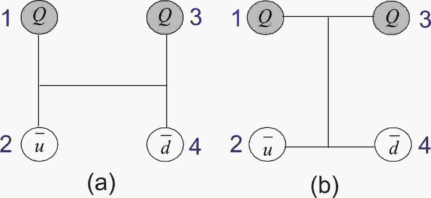
For the
$ T_{QQ}\; (Q = c, b) $ system, there are two quark configurations—the meson–meson structure (MM) and the diquark–antidiquark structure (DA)—which are shown in Fig. 1. Both structures and their coupling effects are considered in this work.
Figure 1. (color online) Two types of configuration of
$ T_{QQ}\; (Q = c, b) $ . Figure (a) represents the meson–meson structure; figure (b) is the diquark–antidiquark structure.The wave functions of tetraquark states should be a product of spin, flavor, color and space degrees of freedom. For the spin component, we denote α and β as the spin-up and spin-down states of quarks, and the spin wave functions for the two-quark system are
$ \begin{aligned}[b] \chi_{11} =& \alpha\alpha,\; \; \chi_{10} = \frac{1}{\sqrt{2}}(\alpha\beta+\beta\alpha),\; \; \chi_{1-1} = \beta\beta, \\ \chi_{00} =& \frac{1}{\sqrt{2}}(\alpha\beta-\beta\alpha), \end{aligned} $

(14) then total six wave functions of the four-body system are obtained, which are shown in Table 3. The subscript of χ represents the spin values
$ S_1 $ and$ S_2 $ of two sub-clusters. The superscript of χ stands for the total spin S ($ S_1 \otimes S_2 $ = S) and the third projection$ M_S $ of S for the four-quark system.Spin Flavor Color $ \chi_{00}^{00}=\chi_{00}\chi_{00} $ 

$ \chi^{00}=-\dfrac{1}{2}(c\bar{d}c\bar{u}-c\bar{u}c\bar{d}) $ 

$ 1 \otimes 1: \chi^{c1}=\dfrac{1}{3}(\bar{r}r+\bar{g}g+\bar{b}b)(\bar{r}r+\bar{g}g+\bar{b}b) $ 

$ \chi_{11}^{00}=\sqrt{\dfrac{1}{3}}(\chi_{11}\chi_{1-1}-\chi_{10}\chi_{10}+\chi_{1-1}\chi_{11}) $ 

$ \chi^{10}=-\dfrac{1}{2}(c\bar{d}c\bar{u}+c\bar{u}c\bar{d}) $ 

$\begin{aligned}[b] 8 \otimes 8: \chi^{c2}=&\frac{\sqrt{2}}{12}(3\bar{b}r\bar{r}b+3\bar{g}r\bar{r}g+3\bar{b}g\bar{g}b+3\bar{g}b\bar{b}g+3\bar{r}g\bar{g}r \\ &+3\bar{r}b\bar{b}r+2\bar{r}r\bar{r}r+2\bar{g}g\bar{g}g+2\bar{b}b\bar{b}b-\bar{r}r\bar{g}g \\ & -\bar{g}g\bar{r}r-\bar{b}b\bar{g}g-\bar{b}b\bar{r}r-\bar{g}g\bar{b}b-\bar{r}r\bar{b}b)\end{aligned}$ 

$ \chi_{01}^{11}=\chi_{00}\chi_{11} $ 

$ \begin{aligned}[b]\bar{3} \otimes 3: \chi^{c3}=&\frac{\sqrt{3}}{6}(rg\bar{r}\bar{g}-rg\bar{g}\bar{r}+gr\bar{g}\bar{r}-gr\bar{r}\bar{g} \\ &+rb\bar{r}\bar{b}-rb\bar{b}\bar{r}+br\bar{b}\bar{r}-br\bar{r}\bar{b} \\ &+gb\bar{g}\bar{b}-gb\bar{b}\bar{g}+bg\bar{b}\bar{g}-bg\bar{g}\bar{b})\end{aligned}$ 

$ \chi_{10}^{11}=\chi_{11}\chi_{00} $ 

$\begin{aligned}[b]6 \otimes \bar{6}: \chi^{c4}=&\frac{\sqrt{6}}{12}(2rr\bar{r}\bar{r}+2gg\bar{g}\bar{g}+2bb\bar{b}\bar{b}+rg\bar{r}\bar{g}+rg\bar{g}\bar{r} \\ &+gr\bar{g}\bar{r}+gr\bar{r}\bar{g}+rb\bar{r}\bar{b}+rb\bar{b}\bar{r}+br\bar{b}\bar{r} \\ &+br\bar{r}\bar{b}+gb\bar{g}\bar{b}+gb\bar{b}\bar{g}+bg\bar{b}\bar{g}+bg\bar{g}\bar{b})\end{aligned}$ 

$ \chi_{11}^{11}=\dfrac{1}{\sqrt{2}}(\chi_{11}\chi_{10}-\chi_{10}\chi_{11}) $ 

$ \chi_{11}^{22}=\chi_{11}\chi_{11} $ 

Table 3. Wave functions of spin, flavor and color for
$ T_{QQ} $ .For the flavor component, the flavor wave functions with isospin
$ = 0 $ and$ 1 $ are also tabulated in Table 3. The subscript$ 00 $ or$ 10 $ of χ represents the total isospin I and the third projection$ I_z $ of I.For the color component, more richer structures in the four-quark system will be considered than conventional
$ q\bar{q} $ mesons and$ qqq $ baryons. For the meson–meson structure in Fig. 1, in the$ SU(3) $ group, the colorless wave functions can be obtained from$ {\bf{1}}\otimes {\bf{1}} = {\bf{1}} $ or$ {\bf{8}} \otimes {\bf{8}} = {\bf{1}} $ . For the diquark–antidiquark structure, the colorless wave functions can be obtained from$ \bar{{\bf{3}}} \otimes {\bf{3}} = {\bf{1}} $ or$ {\bf{6}} \otimes \bar{{\bf{6}}} = {\bf{1}} $ . The detailed expressions of these functions can be found in Table 3.Because the quark contents of the presently investigated four-quark systems are two identical heavy quarks (
$ Q = c, b $ ) and two identical light antiquarks ($ \bar{u}, \bar{d} $ ), the wave functions of$ T_{QQ} $ should satisfy the antisymmetry requirement. Then we collect all the color–spin bases of$ T_{QQ} $ states for possible quantum numbers according to the constraint from the Pauli principle in Table 4.$ I(J^P) $ 

$ 1(0^+) $ 

$ 1(1^+) $ 

$ 1(2^+) $ 

$ 0(1^+) $ 

Bases $ [(c\bar{u})^0_1(c\bar{d})^0_1]^0 $ 

$ [(c\bar{u})^0_1(c\bar{d})^1_1]^1 $ 

$ [(c\bar{u})^1_1(c\bar{d})^1_1]^2 $ 

$ [(c\bar{u})^0_1(c\bar{d})^1_1]^1 $ 

$ [(c\bar{u})^0_8(c\bar{d})^0_8]^0 $ 

$ [(c\bar{u})^0_8(c\bar{d})^1_8]^1 $ 

$ [(c\bar{u})^1_8(c\bar{d})^1_8]^2 $ 

$ [(c\bar{u})^0_8(c\bar{d})^1_8]^1 $ 

$ [(c\bar{u})^1_1(c\bar{d})^1_1]^0 $ 

$ [(c\bar{u})^1_1(c\bar{d})^0_1]^1 $ 

$ [(cc)^1_{\bar{3}}(\bar{u}\bar{d})^1_3]^2 $ 

$ [(c\bar{u})^1_1(c\bar{d})^0_1]^1 $ 

$ [(c\bar{u})^1_8(c\bar{d})^1_8]^0 $ 

$ [(c\bar{u})^1_8(c\bar{d})^0_8]^1 $ 

$ [(c\bar{u})^1_8(c\bar{d})^0_8]^1 $ 

$ [(cc)^0_6(\bar{u}\bar{d})^0_{\bar{6}}]^0 $ 

$ [(cc)^1_{\bar{3}}(\bar{u}\bar{d})^1_3]^1 $ 

$ [(c\bar{u})^1_1(c\bar{d})^1_1]^1 $ 

$ [(cc)^1_{\bar{3}}(\bar{u}\bar{d})^1_3]^0 $ 

$ [(c\bar{u})^1_8(c\bar{d})^1_8]^1 $ 

$ [(cc)^0_6(\bar{u}\bar{d})^1_{\bar{6}}]^1 $ 

$ [(cc)^1_{\bar{3}}(\bar{u}\bar{d})^0_3]^1 $ 

Table 4. Color–spin bases for
$ T_{cc} $ system. The bases can be read as the notation:$ [(c\bar{u})^{S1}_{c1}(c\bar{d})^{S2}_{c2}]^S $ for meson–meson structures,$ [(cc)^{S1}_{c1}(\bar{u}\bar{d})^{S2}_{c2}]^S $ for diquark–antidiquark structures. The superscripts$ S_1 $ ,$ S_2 $ represent the spin for two sub-clusters;$ S\; (S_1 \otimes S_2 = S) $ is the total spin of the four-quark states. The subscripts$ c_1 $ and$ c_2 $ stand for color. For$ T_{bb} $ states, replace c quark with b quark.Next, we discuss the orbital wave functions for a four-body system. These can be obtained by coupling the orbital wave function for each relative motion of the system:
$ \Psi_{L}^{M_{L}} = \left[[\Psi_{l_1}({\boldsymbol r}_{12})\Psi_{l_2}({\boldsymbol r}_{34})]_{l_{12}}\Psi_{L_r}({\boldsymbol r}_{1234}) \right]_{L}^{M_{L}}, $

(15) where
$ l_1 $ and$ l_2 $ are the angular momentum of two sub-clusters.$ \Psi_{L_r}({\boldsymbol{r}}_{1234}) $ is the wave function of the relative motion between the two sub-clusters with orbital angular momentum$ L_r $ . L is the total orbital angular momentum of the four-quark state. In the present work, we only consider the low-lying S-wave double heavy tetraquark states, so it is natural to assume that all the orbital angular momenta are zero. In GEM, the spatial wave functions are expanded in series of Gaussian basis functions:$ \Psi_{l}^{m}({\boldsymbol{r}}) = \sum\limits_{n = 1}^{n_{\max}} c_{n}\psi^G_{nlm}({\boldsymbol{r}}), $

(16) $ \psi^G_{nlm}({\boldsymbol{r}}) = N_{nl}r^{l} {\rm e}^{-\nu_{n}r^2}Y_{lm}(\hat{{\boldsymbol{r}}}),$

(17) where
$ N_{nl} $ are normalization constants,$ N_{nl} = \left[\frac{2^{l+2}(2\nu_{n})^{l+\frac{3}{2}}}{\sqrt{\pi}(2l+1)} \right]^{{1}/{2}},$

(18) $ c_n $ are the variational parameters, which are determined dynamically. The Gaussian size parameters are chosen according to the following geometric progression:$ \nu_{n} = \dfrac{1}{r^2_n}, \quad r_n = r_1a^{n-1}, \quad a = \left(\dfrac{r_{n_{\max}}}{r_1}\right)^{{1}/({n_{\max}-1})}. $

(19) This procedure enables optimization of the expansion using just a small number of Gaussian functions. Then, the complete channel wave function
$ \Psi^{\,M_IM_J}_{IJ} $ for the four-quark system is obtained by coupling the orbital and spin, flavor, and color wave functions obtained in Table 4. Finally, the eigenvalues of the four-quark system are obtained by solving the Schrödinger equation:$ H \, \Psi^{\,M_IM_J}_{IJ} = E^{IJ} \Psi^{\,M_IM_J}_{IJ}. $

(20) -
In the present work, we are interested in looking for the bound states of low-lying S-wave
$ T_{QQ}\; (Q = c, b) $ system. The allowed quantum numbers are$ I(J^P) = $ $ 1(0^+), 1(1^+), 1(2^+), 0(1^+) $ under the constraints of the Pauli principle. The possible resonances of these states are searched with the help of the real scaling method (RSM). For bound state calculations, we aim to study the influence of the color structures on the binding energy. -
The low-lying eigenvalues of iso-vector
$ T_{QQ} $ states with$ I(J^P) = 1(0^+), 1(1^+), 1(2^+) $ are shown in Table 5. From the table, we can see that the low-lying energies are all higher than the corresponding theoretical thresholds, no matter whether in a meson–meson structure, a diquark–antidiquark structure or even considering the coupling of the two structures. No bound states are found.$ I(J^P) $ 

MM DA $ E_{cc} $ 

$E_{\rm Theo}$ 

$E_{\rm Exp}$ 

$ T_{cc} $ 

$ 1(0^+) $ 

3726.8 4086.6 3726.7 3725.2 ( $ D^0D^+ $ )

3734.4 $ 1(1^+) $ 

3844.8 4133.3 3844.7 3843.2 ( $ D^0D^{*+} $ )

3871.8 $ 1(2^+) $ 

3962.8 4159.4 3962.7 3961.2 ( $ D^{*0}D^{*+} $ )

4017.3 $ T_{bb} $ 

$ 1(0^+) $ 

10562.3 10730.2 10562.3 10561.6 ( $ B^{-}\bar{B}^0 $ )

10558.5 $ 1(1^+) $ 

10601.2 10741.1 10601.1 10600.4 ( $ B^{-}\bar{B^*}^0 $ )

10604.5 $ 1(2^+) $ 

10639.9 10751.6 10639.9 10639.2 ( $ B^{*-}\bar{B^*}^0 $ )

10650.5 Table 5. Low-lying eigenvalues of iso-vector
$ T_{QQ} $ states with$ I(J^P) = 1(0^+), 1(1^+), 1(2^+) $ (in units of MeV). MM and DA represent the meson–meson structures and diquark–antidiquark structures, respectively.$ E_{cc} $ is the energy considering the coupling of MM and DA.$ E_{\rm Theo} $ and$ E_{\rm Exp} $ is the theoretical and experimental threshold.Table 6 and Table 7 give the mass of iso-scalar
$ T_{cc} $ and$ T_{bb} $ with$ I(J^P) = 0(1^+) $ . The first column is the color–spin channel (listed in Table 4). The second column refers to the color structure including$ 1\times1 $ ,$ 8\times8 $ and their mixing, as well as$ \bar{3}\times3 $ ,$ 6\times \bar{6} $ and their mixing. The following two columns represent the theoretical mass (E) and theoretical thresholds ($ E_{\rm Theo} $ ). The last column gives the binding energy$ \Delta E = E-E_{\rm Theo} $ . In Table 6, we find that there are no bound states in the single-channel calculation except for the diquark–antidiquark$ \bar{3}\times 3 $ structure. When considering the coupling of$ 1\times 1 $ and$ 8 \times 8 $ color structures in the meson–meson configuration, a loosely bound state with mass$ M = 3841.4 $ MeV is obtained with the binding energy 1.8 MeV, which is consistent with the recent experiment data from LHCb. In diquark–antidiquark coupling calculations, a tightly bound state with mass$ M = 3700.9 $ MeV is obtained with the binding energy 142.3 MeV. We obtain the lowest state with mass$ M = 3660.7 $ MeV, a tightly bound state with binding energy 182.5 MeV, by considering the complete channel coupling effects including both meson–meson and diquark–antidiquark structures.Channel color structure E $ E_{\rm Theo} $ 

$ \Delta E $ 

$ [(c\bar{u})^0_1(c\bar{d})^1_1]^1 $ 

$ 1\times1 $ 

3843.8 3843.2 ( $ D^0D^{*+} $ )

+0.6 $ [(c\bar{u})^0_8(c\bar{d})^1_8]^1 $ 

$ 8\times8 $ 

4168.7 +325.5 $ 1\times1 $ +

$ 8\times8 $ 

3842.0 −1.2 $ [(c\bar{u})^1_1(c\bar{d})^0_1]^1 $ 

$ 1\times1 $ 

3843.8 3843.2 ( $ D^{*0}D^{+} $ )

+0.6 $ [(c\bar{u})^1_8(c\bar{d})^0_8]^1 $ 

$ 8\times8 $ 

4168.7 +325.5 $ 1\times1 $ +

$ 8\times8 $ 

3842.0 −1.2 $ [(c\bar{u})^1_1(c\bar{d})^1_1]^1 $ 

$ 1\times1 $ 

3961.9 3961.2 ( $ D^{*0}D^{*+} $ )

+0.7 $ [(c\bar{u})^1_8(c\bar{d})^1_8]^1 $ 

$ 8\times8 $ 

4102.3 +141.1 $ 1\times1 $ +

$ 8\times8 $ 

3958.7 −2.5 all $ 1\times 1 $ mixing

3841.7 3843.2 ( $ D^0D^{*+} $ )

−1.5 MM structure mixing 3841.4 3843.2 ( $ D^0D^{*+} $ )

−1.8 $ [(cc)^0_6(\bar{u}\bar{d})^1_{\bar{6}}]^1 $ 

$ 6\times \bar{6} $ 

4115.1 3843.2 ( $ D^0D^{*+} $ )

+271.9 $ [(cc)^1_{\bar{3}}(\bar{u}\bar{d})^0_3]^1 $ 

$ \bar{3}\times 3 $ 

3704.8 −138.4 DA structure mixing 3700.9 −142.3 MM and DA mixing 3660.7 3843.2 ( $ D^0D^{*+} $ )

−182.5 Table 6. Mass of iso-scalar
$ T_{cc} $ states with$ I(J^P) = 0(1^+) $ (in units of MeV).Channel color structure E $E_{\rm Theo}$ 

$ \Delta E $ 

$ [(b\bar{u})^0_1(b\bar{d})^1_1]^1 $ 

$ 1\times1 $ 

10590.3 10600.4 ( $ B^{-}\bar{B^*}^0 $ )

−10.1 $ [(b\bar{u})^0_8(b\bar{d})^1_8]^1 $ 

$ 8\times8 $ 

10765.7 +165.3 $ 1\times1 $ +

$ 8\times8 $ 

10566.7 −33.7 $ [(b\bar{u})^1_1(b\bar{d})^0_1]^1 $ 

$ 1\times1 $ 

10590.3 10600.4 ( $ B^{*-}\bar{B}^0 $ )

−10.1 $ [(b\bar{u})^1_8(b\bar{d})^0_8]^1 $ 

$ 8\times8 $ 

10765.7 +165.3 $ 1\times1 $ +

$ 8\times8 $ 

10566.7 −33.7 $ [(b\bar{u})^1_1(b\bar{d})^1_1]^1 $ 

$ 1\times1 $ 

10629.8 10639.2 ( $ B^{*-}\bar{B^*}^0 $ )

−9.4 $ [(b\bar{u})^1_8(b\bar{d})^1_8]^1 $ 

$ 8\times8 $ 

10738.5 +99.3 $ 1\times1 $ +

$ 8\times8 $ 

10598.8 −40.4 all $ 1\times 1 $ mixing

10551.8 10600.4 ( $ B^{-}\bar{B^*}^0 $ )

−48.6 MM structure mixing 10545.9 10600.4 ( $ B^{-}\bar{B^*}^0 $ )

−54.5 $ [(bb)^0_6(\bar{u}\bar{d})^1_{\bar{6}}]^1 $ 

$ 6\times \bar{6} $ 

10746.8 10600.4 ( $ B^{-}\bar{B^*}^0 $ )

+146.4 $ [(bb)^1_{\bar{3}}(\bar{u}\bar{d})^0_3]^1 $ 

$ \bar{3}\times 3 $ 

10298.9 −301.5 DA structure mixing $ 10298.2 $ 

−302.2 $ 10576.8 $ 

-23.6 MM and DA mixing $ 10282.7^{1st} $ 

10600.4 ( $ B^{-}\bar{B^*}^0 $ )

−317.7 $ 10516.7^{2nd} $ 

−83.7 Table 7. Mass of iso-scalar
$ T_{bb} $ states with$ I(J^P) = 0(1^+) $ (in units of MeV).The same calculations are extended to the
$ T_{bb} $ system in Table 7. With the increase of$ m_{Q} $ , the bound states are easier to obtain. When considering the single channel, for$ 1 \times 1 $ and$ \bar{3} \times 3 $ color structures, there are bound states, except for$ 8 \times 8 $ and$ 6 \times \bar{6} $ color structures. The mixing of the meson–meson structure leads to a bound state at 10545.9 MeV, which has 54.5 MeV binding energy. The mixing of diquark–antidiquark structures obtains a deeper bound state. When considering the coupling of meson–meson and diquark–antidiquark structures, we find two bound states with masses 10282.7 and 10516.7 MeV.We compare our results with some recent calculations in Table 8. From the table, we can see that for
$ T_{cc} $ of$ 0(1^+) $ , there is controversy as to whether there are bound states. Our one shallow bound state with binding energy 1.8 MeV is consistent with Refs. [21, 26, 40], also in the case where only meson-meson structures are considered. In lattice QCD calculations, a few works support a bound state, also with small binding energy [52]. If one considers diquark–antidiquark structures in the calculations, a deeper bound state for$ T_{cc} $ of$ 0(1^+) $ is also obtained, as in Refs. [23, 35]. For$ T_{bb} $ of$ 0(1^+) $ , the situation becomes much clearer. Almost all works obtained bound results. In the case of considering the meson–meson structures, our result with binding energy 54.5 MeV is consistent with Refs. [21, 24] in the quark model and also Ref. [49] in the lattice QCD calculation. No matter for$ T_{cc} $ or$ T_{bb} $ , when diquark–antidiquark structures are taken into account, deeper binding energies will appear, which seems to be somewhat misleading. In some other works, the same conclusions are obtained, such as in Refs. [12, 14, 29, 31].$ T_{cc} $ 

This work [11] [13] [15] [18] [19] [21] [23] [24] [25] [26] [31] [33] [34] [35] [40] [48] [52] −1.8 (MM) −79 −96 −98 N N −1 −182.3 N N −1 −23 N N −150 −3 N −23.3±11.4 −142.3 (DA) −182.5 (MM+DA) $ T_{bb} $ 

This work [15] [18] [20] [21] [22] [23] [24] [25] [31] [33] [34] [35] [49] [51] [52] [53] [55] −54.5 (MM) −268.6 −215 −150 −35 −120.9 −317 −54 −102 −173 N −145 −278 −30 ~ -57 −189±13 −143.3±34 −128±24±10 −167±19 −302.2 (DA) $ -317.7^{1st} $ (MM+DA)

$ -83.7^{2nd} $ (MM+DA)

Table 8. Results for
$ T_{cc} $ and$ T_{bb} $ tetraquarks with$ 0(1^+) $ in comparison with the other theoretical calculations (in units of MeV). N stands for "no bound state". In the second column, (MM) represents only meson–meson structures considered, (DA) stands for only diquark–antidiquark configurations, and (MM+DA) represents the coupling of meson–meson and diquark–antidiquark structures.In order to understand the mechanism of forming the bound states for different color structures and their couplings, the contributions of each term in the Hamiltonian for
$ T_{cc} $ with$ 0(1^+) $ are given in Table 9. In the table,$ K_1 $ and$ K_2 $ are the kinetic energy of the two sub-clusters, and$ K_3 $ represents the relative kinetic energy between these two clusters.$ V^{\rm{C, Coul, CMI}} $ refer to confinement (C), color Coulomb (Coul), and color–magnetic interaction (CMI).$ V^{\eta, \pi, \sigma} $ represent pseudoscalar meson η, π exchange and scalar meson σ exchange. To understand the mechanism, one has to compare the results in the tetraquark calculation to those of two free mesons which are listed in the last column in Table 9. For color singlet channels (index 1, 3, 5), the attractions provided by π and σ are too weak to overcome the relative kinetic energy to bind two color singlet clusters together, and these channels are scattering states when they stand alone. Coupling these color singlet channels adds more attraction, and a shallow bound state is formed (see the column headed by 1+3+5). The effect of coupling color octet–octet channels is very small, adding$ 0.3 $ MeV to the binding energy (see the column headed by MM). If only the meson–meson structure is considered, the reported result from the LHCb collaboration can be explained by the molecular state. However, for a multi-quark system, more color structures are possible, in which the diquark–antidiquark structure with color representations$ \bar{3} \times 3 $ and$ 6 \times \bar{6} $ are often invoked. For the$ \bar{3} \times 3 $ channel (column headed by 8), the strong attractions from π meson exchange, σ meson exchange and CMI overcome the repulsion from the kinetic energy and bind two "good diquark/antidiquark" [75] to form a deep bound state. The channel coupling between$ \bar{3} \times 3 $ and$ 6 \times \bar{6} $ channels adds a little more binding energy to the system. The attraction from π-meson exchange in "good diquark" is very large because of its compact structure, as does the color magnetic interaction. The calculations without invoking pseudoscalar exchange do not obtain a bound state of$ T_{cc} $ [17], supporting this statement.Channel 1 2 3 4 5 6 7 8 $ 1+3+5 $ 

MM DA MM+DA $ D^0+D^{*+} $ 

$ K_1 $ 

516.8 317.2 359.8 322.8 359.6 347.3 119.4 191.2 442.2 440.2 192.2 321.8 516.7 $ K_2 $ 

359.8 322.8 516.8 317.2 359.6 347.3 295.4 1052.2 442.2 440.2 1050.6 929.7 359.3 $ K_3 $ 

3.4 307.3 3.4 307.3 3.0 323.4 395.4 262.3 17.4 25.5 267.0 189.9 0 $ V^{\rm{C}} $ 

−390.4 −264.2 −390.4 −264.2 −335.8 −300.8 −271.2 −412.9 −393.1 −393.6 −415.6 −432.8 −390.0 $ V^{\rm{Coul}} $ 

−612.9 −517.8 −612.9 −517.8 −543.8 −539.1 −506.4 −621.6 −614.8 −614.7 −623.6 −645.8 −612.7 $ V^{\rm{CMI}} $ 

−113.1 −6.6 −113.1 −6.6 38.7 −77.9 −6.8 −350.6 −118.7 −120.1 −356.7 −346.4 −112.1 $ V^{\eta} $ 

0 5.5 0 5.5 0 6.5 −2.5 86.7 0.9 1.1 86.2 75.4 0 $ V^{\pi} $ 

−0.5 −56.9 −0.5 −56.9 −0.4 −63.9 28.3 −530.6 −10.8 −12.9 −527.4 −464.6 0 $ V^{\sigma} $ 

−1.3 −20.5 −1.3 −20.5 −1.1 −22.2 −18.5 −53.8 −5.6 −6.1 −53.8 −48.8 0 E 3843.8 4168.7 3843.8 4168.7 3961.9 4102.3 4115.1 3704.8 3841.7 3841.4 3700.9 3660.7 3843.2 $ \Delta E $ 

+0.6 +325.5 +0.6 +325.5 +0.7 +141.1 +271.9 −138.4 −1.5 −1.8 −142.3 −182.5 0 Table 9. Contributions of each potential in the system Hamiltonian of
$ T_{cc} $ with$ I(J^P) = 0(1^+) $ for different color structures and their couplings (in units of MeV). In the first row, to save space, we give labels in the sequence 1 ~ 8 for the eight channels of$ T_{cc} $ with$ 0(1^+) $ , as listed in Table 4.From quantum mechanics, one knows that the physical states are the linear combinations of all possible channels in various structures. So channel coupling with inclusion of different structures is needed. Clearly, the effect of this channel coupling will push the lowest state down further. A deep bound state with binding energy 182.5 MeV appears. Unfortunately, the shallow bound state in the meson–meson structure is pushed up above the threshold and so disappears. Experimentally, if there is only one weekly bound
$ T_{cc} $ state, diquark–antidiquark configurations should be abandoned, or the quark–quark interaction in the diquark structure should be modified with the accumulation of experimental data.In the discussion of hadronic states, the electromagnetic interaction is almost neglected due to the small coupling constant
$ \alpha \approx 1/137 $ . However, for the weakly bound state,$ E_{B}/M << 1 $ , the electromagnetic interaction may play a role. To investigate the role of the electric Coulomb force, we add the Coulomb potential$ \alpha\dfrac{q_iq_j}{r_{ij}} $ to the system Hamiltonian and solve the Schrödinger equation in the same way as above. The results show that the states are stable against the inclusion of the electric Coulomb interaction. The lowest eigen-energies are changed to 3840.7, 3700.2 and 3660.2 MeV in the MM structure, the DA structure and structure mixing respectively.In order to learn about the nature of doubly-heavy tetraquark states, we calculate the distances between any quark and quark/antiquark, which are shown in Table 10. We need to note that, for
$ T_{QQ} $ , because the heavy quarks Q are identical particles, as well as the light antiquark$ \bar{u} $ and$ \bar{d} $ , the distance$ r_{12} $ in the Table 10 actually is not the real value between the first quark Q and the second antidiquark$ \bar{u} $ . It should be the average:$ I(J^P) $ 

$ T_{cc} $ 

$ T_{bb} $ 

Resonance states Γ Resonance states Γ $ 1(0^+) $ 

... ... 11309 23 $ 1(1^+) $ 

4639 10 11210 62 11318 21 $ 1(2^+) $ 

4687 9 11231 73 11329 0.4 $ 0(1^+) $ 

4304 38 10641 2 Table 10. The decay widths of predicted resonances of
$ T_{cc} $ and$ T_{bb} $ systems. (unit: MeV).$ \begin{aligned}[b] r_{12}^2= &r_{34}^2 = r_{14}^2 = r_{23}^2 \\ =& \frac{1}{4}(r_{Q^1\bar{u}^2}^2+r_{Q^1\bar{d}^4}^2+r_{Q^3\bar{u}^2}^2+ r_{Q^3\bar{d}^4}^2 ). \end{aligned} $

(21) The numbers '1,2,3,4' are as shown in Fig. 1. From the table, for the weakly bound state of
$ T_{cc} $ with mass$ 3841.4 $ MeV, with just the meson–meson structure considered, the distance$ r_{13} $ and$ r_{24} $ between two sub-clusters is larger than the distance within one cluster, which indicates that it is a molecular$ DD^* $ state. On the contrary, the tightly bound states 3700.9 and 3660.7 MeV are diquark–antidiquark structures. Furthermore, from the table we can see that although the$ \bar{u}\bar{d} $ is a good diquark, its size is sightly larger than that of the$ cc $ diquark. This should be from the color–electric interaction, not the color–magnetic interaction. -
In our work, we are also concerned about the possible resonance states of iso-vector and iso-scalar
$ T_{QQ} $ . To find the genuine resonances, the dedicated real scaling (stabilization) method is employed. In our previous work [76], this method was used successfully to explain the$ Z_{cs}(3985) $ observed by the BESIII collaboration [77]. To realize the real scaling method in our calculation, we need to multiply by a factor α the Gaussian size parameter$ r_n $ in Eq. (19) just for the meson–meson structure with color singlet–singlet configuration. In our calculation, α takes values from 1.0 to 3.0. With the increase of α, all states will fall off towards their thresholds, but bound states should be stable and resonances will appear as an avoid-crossing structure as in Fig. 2 [78]. In the figure, at the avoid-crossing structure, there are two lines. The upper line is a scattering state with larger slope, which will fall down to the threshold. The lower line represents the resonance state, which tries to keep stable with a smaller slope. When the resonance state and the scattering state interact with each other, this brings about an avoid-crossing point as in Fig. 2. With the increase of the scaling factor α, the energy of the other higher scattering state will fall down, will interact with this resonance state again and another avoid-crossing point will emerge. In our work, we set the number of repetitions of avoid-crossing points to 2, owing to the large amount of computation required. Theoretically speaking, with the continuous increase of α, avoid-crossing points will appear in succession. Then we have found a resonance state. For bound states, with the increase of α, they always stay stable. We show the results for the$ T_{QQ} $ system with all possible quantum numbers in Figs. 3–10 by considering the complete channel couplings.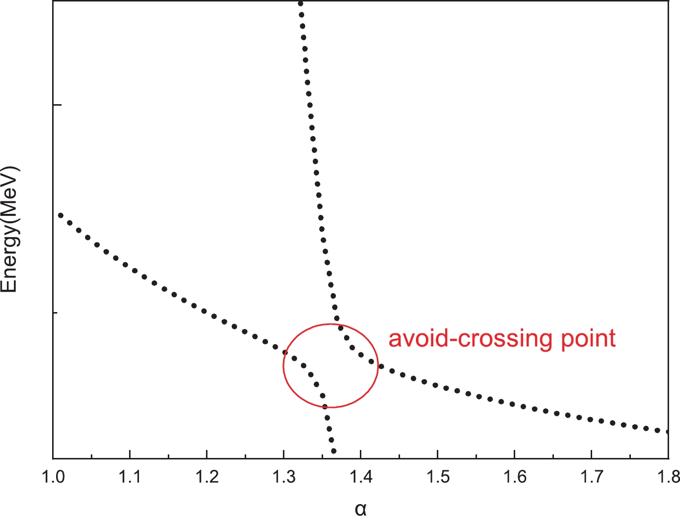
Figure 2. (color online) Stabilization graph for the resonance.

Figure 3. (color online) Stabilization plots of the energies of
$ T_{cc} $ states for$ I(J^P) = 1(0^+) $ with respect to the scaling factor α.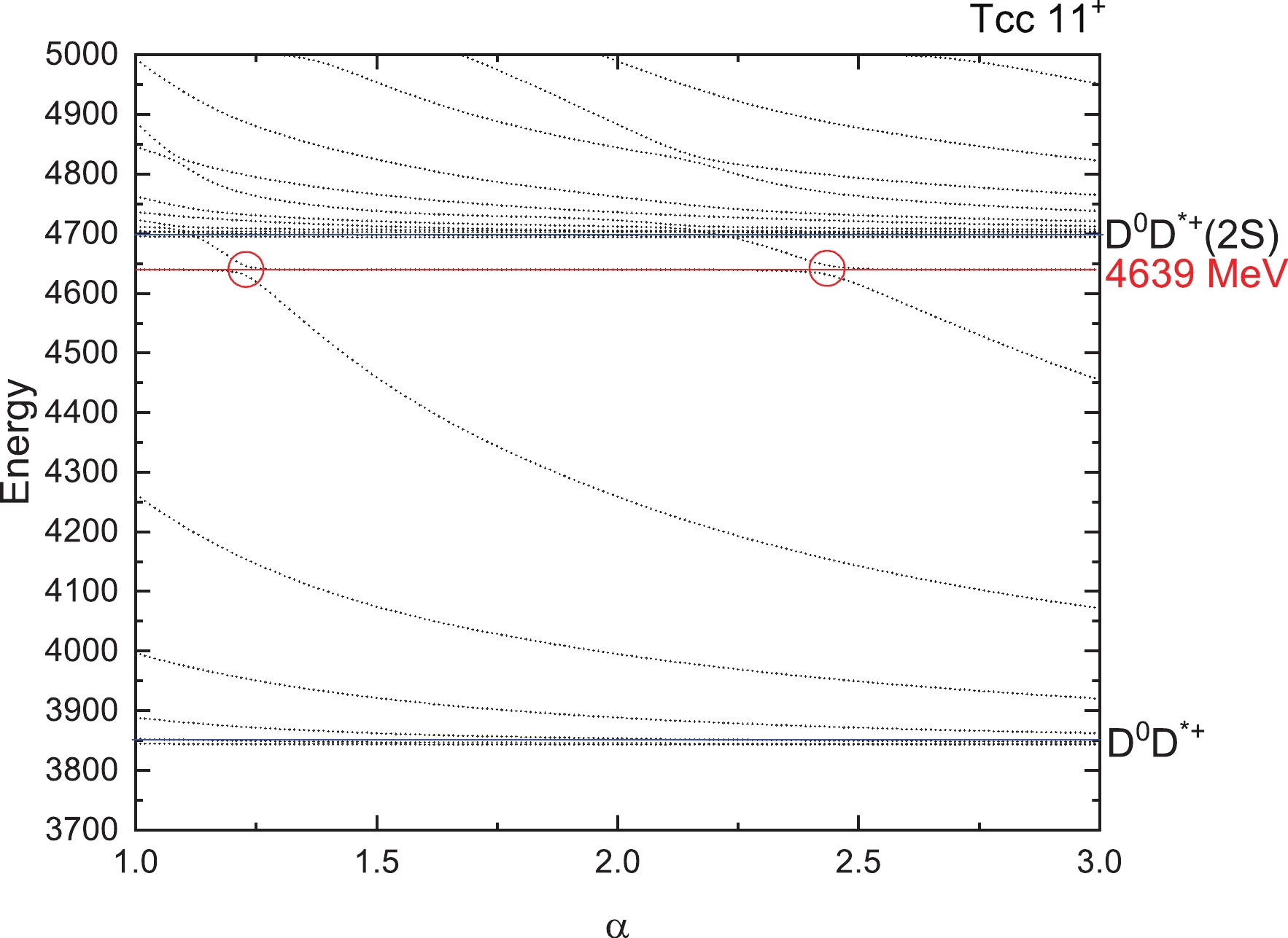
Figure 4. (color online) Stabilization plots of the energies of
$ T_{cc} $ states for$ I(J^P) = 1(1^+) $ with respect to the scaling factor α.
Figure 5. (color online) Stabilization plots of the energies of
$ T_{cc} $ states for$ I(J^P) = 1(2^+) $ with respect to the scaling factor α.
Figure 6. (color online) Stabilization plots of the energies of
$ T_{cc} $ states for$ I(J^P) = 0(1^+) $ with respect to the scaling factor α.
Figure 7. (color online) Stabilization plots of the energies of
$ T_{bb} $ states for$ I(J^P)=1(0^+) $ with respect to the scaling factor α.
Figure 8. (color online) Stabilization plots of the energies of
$ T_{bb} $ states for$ I(J^P)=1(1^+) $ with respect to the scaling factor α.
Figure 9. (color online) Stabilization plots of the energies of
$ T_{bb} $ states for$ I(J^P)=1(2^+) $ with respect to the scaling factor α.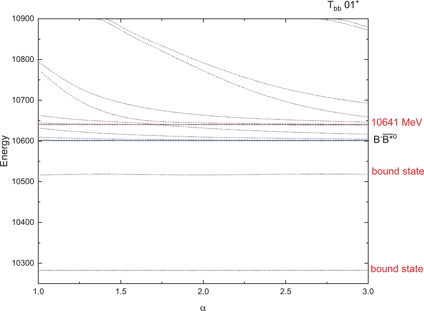
Figure 10. (color online) Stabilization plots of the energies of
$ T_{bb} $ states for$ I(J^P)=0(1^+) $ with respect to the scaling factor α.Figure 3 represents the
$ T_{cc} $ states for$ 1(0^+) $ . The four horizontal blue lines are the thresholds of$ D^0D^+ (0 \otimes $ $ 0 \rightarrow 0) $ ,$ D^{*0}D^{*+} (1 \otimes 1 \rightarrow 0) $ and their excited states$ D^0D^+(2S) $ and$ D^{*0}D^{*+}(2S) $ . Higher energies are not listed here. We found no resonances for this state. From Fig. 4, two thresholds$ D^0D^{*+} $ and its excited states$ D^0D^{*+}(2S) $ appear clearly. Around an energy of 4639 MeV, we found the avoid-crossing phenomenon, which represents a genuine resonance state. In Fig. 5, we can see that the energy of the lowest resonance state is about 4687 MeV for$ T_{cc} $ with$ 1(2^+) $ . For iso-scalar$ T_{cc} $ with$ 0(1^+) $ , a bound state with mass 3660 MeV is obtained and the lowest resonance state shows with a stable energy of 4304 MeV in Fig. 6.For iso-vector and iso-scalar
$ T_{bb} $ states, there are also some resonance states found. They are states with masses of 11309 MeV for$ 1(0^+) $ , 11210 and 11318 MeV for$ 1(1^+) $ , 11231 and 11329 MeV for$ 1(2^+) $ , and 10641 MeV for$ 0(1^+) $ . There may be more resonance states with higher energies, which may be too wide to observe or too difficult to produce. So in our work, we only give the resonance states with energies as low as possible.Furthermore, we calculated the decay widths of these resonance states using the formula taken from Reference [78]:
$ \Gamma = 4|V(\alpha)|\frac{\sqrt{|S_r||S_c|}}{|S_c-S_r|}, $

(22) where
$ V(\alpha) $ is the difference between the two energies at the avoid-crossing point with the same value α, and$ S_r $ and$ S_c $ are the slopes of the scattering line and resonance line, respectively. For each resonance, we obtain the values of the decay width at the first and the second avoid-crossing point, and then we give the average decay width of these two values. The results are shown in Table 10. It should be noted that the decay width is the partial strong two-body decay width to S-wave channels included in the calculation. For example, for$ T_{cc} $ of$ 1(1^+) $ , there is a resonance state with energy 4639 MeV, which has the decay width of 10 MeV in Table 10. This decay value is just the partial width to the$ D^0D^{*+} $ channel (see the threshold in Fig. 4). For$ T_{cc} $ of$ 0(1^+) $ , the decay width of resonance (4304) with 38 MeV is the partial decay to$ D^{*0}D^{*+} $ ,$ D^0D^{*+} $ and$ D^{+}D^{*0} $ channels (see the thresholds in Fig. 6). -
In the framework of the chiral quark model, we undertake a systematic calculation for the mass spectra of doubly-heavy
$ T_{QQ} $ with quantum numbers$ I(J^P) = 1(0^+), 1(1^+), 1(2^+),\; 0(1^+) $ , to look for possible bound states. Also, some resonance states are found with the real scaling method.In bound state calculations, we analyze the effects of different color structures, such as
$ 1 \times 1 $ ,$ 8 \times 8 $ for meson–meson structures and$ \bar{3} \times 3 $ ,$ 6 \times \bar{6} $ for diquark–antidiquark structures, on the binding energy of$ T_{QQ} $ . The masses of states with isospin$ I = 1 $ are all above the corresponding thresholds, leaving no space for bound states. For$ T_{cc} $ with$ 0(1^+) $ , we find that in the meson–meson structure, a loosely bound state at 3841.1 MeV is obtained with a$ 1.8 $ MeV binding energy, which is consistent with the recent observed experiment at LHCb. But in diquark–antidiquark structures, CMI potential, π-exchange and σ exchange offer more attractions and a tightly bound state with mass 3700 MeV is obtained. The couplings of meson–meson and diquark–antidiquark structures can not be neglected, which leads to more deeper bound states and destroys the loosely bound state. For the heavier$ T_{bb} $ system with$ 0(1^+) $ , the same conclusions are obtained, similar to the case of$ T_{cc} $ , and it looks easier to find more deeper bound states. For example, a bound state 10545.9 MeV with binding energy 54.5 MeV is obtained when only meson–meson structures are considered. If only diquark–antidiquark structures are taken into account, two bound states emerge with binding energy 302.2 MeV and 23.6 MeV. When considering the coupling of meson–meson and diquark–antidiquark configurations, these two states will have deeper binding energies of 317.7 MeV and 83.7 MeV.For resonance state calculations, some resonances are found. For
$ T_{cc} $ , the energies of the possible resonances are 4639 MeV for$ 1(1^+) $ , 4687 MeV for$ 1(2^+) $ , 4304 MeV for$ 0(1^+) $ . For$ T_{bb} $ , the resonance energies are larger than$ T_{cc} $ , which takes 11309 MeV for$ 1(0^+) $ , 11210 and 11318 MeV for$ 1(1^+) $ , 11231 and 11329 MeV for$ 1(2^+) $ , 10641 MeV for$ 0(1^+) $ . Hopefully, our results in this work by the phenomenological framework of the chiral quark model may be confirmed in future high energy experiments.
Doubly-heavy tetraquark states ${\boldsymbol c \boldsymbol c\bar{\boldsymbol u}\bar{\boldsymbol d}} $ and ${\boldsymbol b \boldsymbol b\bar{\boldsymbol u}\bar{\boldsymbol d}} $
- Received Date: 2021-11-23
- Available Online: 2022-05-15
Abstract: Inspired by the recent observation of a very narrow state, called


 DownLoad: