


 Abstract
 HTML
HTML Reference
 Related
 PDF
PDF


-
As the origin of our universe predicted by the standard cosmology model based on classical general relativity (GR), the singular big bang point strongly indicates that it is necessary to introduce a quantum gravity theory to describe the spacetime of the early universe at a small scale. Background independent and nonpertubative loop quantum gravity (LQG) is constructed as one of the candidates for the quantum gravity theory, and it predicts that the spatial geometry is discrete at the Planck scale [1-4]. This discrete geometry feature is inherited in loop quantum cosmology (LQC), which is given by studying the loop quantum states of homogeneous and isotropic geometry [5-7]. The LQC model reproduces the standard Wheeler-DeWitt theory for cosmology at a large scale, while it leads to notable deviations at a small scale because it involves the discreteness of geometry. More explicitly, by applying techniques developed in the full theory of LQG, the classical Hamiltonian constraint in LQC can be reformulated in terms of a new set of variables. Then, the loop quantization procedure is performed to give the quantum Hamiltonian constraint, which takes the formulation as a quantum difference equation so that it evolves non-singularly through the big bang point. Also, it has been pointed out that the metric signature-change at high density is a possible consequence of deformed space-time structures in LQG, which provides a new scenario regarding how singularity-resolution can take place in LQG [8, 9].
The LQC model takes various formulations by following different regularization processes with respect to the Hamiltonian constraint. In standard LQC, the quantization of the Hamiltonian constraint follows a standard method [6]. Note that the Hamiltonian constraint in the full theory of the connection formulation of GR contains the so-called Euclidean term and Lorentzian term, which are classically proportional to each other in the spatial-flat cosmology model. Usually, based on this classical equivalence, the Hamiltonian constraint in standard LQC is simplified before quantization, so that it only contains the quantized Euclidean term [6]. With this simplification, the dynamics governed by the quantum Hamiltonian constraint predicts that the big bang is replaced by a big bounce, which divides the evolution of the universe into two symmetry periods. However, it has been shown that the Euclidean term and Lorentzian term in the Hamiltonian constraint are not proportional to each other in the full theory of LQG [10-12]. By dealing with these two terms separately through Thiemann regularization, a new model of LQC is obtained [10-14]. In this model, quantization of the Hamiltonian constraint gives a new fourth-order difference equation, rather than the second-order one in standard LQC. A remarkable prediction of the dynamics given by the new effective Hamiltonian constraint is that the big bounce divides the evolution of the universe into two non-symmetric periods, with one of the periods being consistent with the evolution described by standard cosmology at a large scale, while the other period is described by a standard cosmology with the presence of a large cosmological constant at a large scale [10, 11].
The amazing result of the new LQC model indicates that the quantum geometry corrections are not only introduced near the region where the singularity appears, but also emerge as an additional cosmology constant in the dynamics equation at a large scale. According to the singularity theorem proved by Hawking and Penrose, singularity is inevitable in GR if the Universe satisfies some energy conditions. Therefore, the bounce in the new LQC model strongly suggests the violation of energy conditions with respect to some effective matter field. In addition, the emergent positive cosmology constant in the de Sitter epoch also contributes to the behavior of energy conditions. It is then natural to ask the following. Which specific energy condition is violated in the new model of LQC? Where does this occur? In the current study, we choose some representative energy conditions, such as average null, strong, and dominant energy conditions, and perform an explicit calculation to analyze the behaviors of the energy conditions with respect to the effective stress-energy tensor given by the effective dynamics equation in the new model of LQC. This task has been discussed in standard LQC as well as in the quantum corrected Schwarzschild-Kruskal space-time [15-19]. It has been shown that, with respect to the effective stress-energy tensor, the average null energy condition is violated in the massless scalar field coupled model, while the strong energy condition is violated only at a small scale in standard LQC. With the new model of LQC introducing the cosmology constant at a large scale as a new feature compared with the standard one, we hope this feature can also be reflected in the behaviors of energy conditions with respect to the effective stress-energy tensor. This is the main goal of this paper.
The following sections of this paper are organized as follows. In Sec. II, we review some basic building blocks of the new LQC model and fix the notations we use in this study. Then, we discuss the violation of energy conditions in Sec. III; we analyze the average null, strong, and dominant energy conditions in different subsections. Conclusions and outlook are provided in the last section.
-
Classically, the flat, homogenous, and isotropic universe that we focus on in this paper is described by the Friedman-Lemaitre-Robertson-Walker (FLRW) metric
$ {\rm d}s^2 = -{\rm d}t^2+a^2({\rm d}x^2+{\rm d}y^2+{\rm d}z^2), $

(1) with
$ a $ being the scale factor of the universe, which only depends on$ t $ , based on the homogeneity assumption of the universe. The dynamics of this system is governed by the Hamiltonian, given by [5-7]$ H_{\rm{cl}} = -\frac{3}{8\pi G\gamma^2}\sqrt{p}c^2+H_{\rm{matter}}(p_\phi,\phi), $

(2) where we use the conjugate variables
$ (c,p) $ defined by$ c: = \gamma\dot{a} $ ,$ p: = a^2 $ , where$ \gamma $ represents the Barbero-Immirzi parameter, and$ H_{\rm{matter}}(p_\phi,\phi) $ is the Hamiltonian of a matter field, with$ \phi $ and$ p_\phi $ representing the matter field and its conjugate momentum, respectively. The pair$ (c,p) $ is usually used to coordinatize the phase space of LQC with the Poisson bracket$ \{c,p\} = \dfrac{8\pi G\gamma}{3} $ . The dynamics equation of classical cosmology is described by the following Friedmann and Raychaudhuri equations as$ H^2 = \frac{8\pi G}{3}\rho, $

(3) $ \frac{\ddot{a}}{a} = \dot{H}+H^2 = -\frac{4\pi G}{3}(\rho_\phi+3P_\phi), $

(4) where
$ H: = \dfrac{\dot{a}}{a} $ is the Hubble parameter;$ \rho_\phi $ and$ P_\phi $ are the energy density and pressure of matter, defined as follows:$ \rho_\phi = a^{-3}H_{\rm{matter}}, $

(5) $ P_\phi = -\frac{1}{3} a^{-2}\frac{\partial H_{\rm{matter}}}{\partial a}, $

(6) with the stress-energy tensor of the matter field taking the form
$ \begin{aligned}[b] T_{\mu\nu} =& \rho_\phi U_\mu U_\nu+P_\phi(g_{\mu\nu}+U_\mu U_\nu){}\\ = &\rho_\phi({\rm d}t)_\mu({\rm d}t)_\nu +a^2P_\phi\left[({\rm d}x)_\mu({\rm d}x)_\nu\right.\\ &+\left.({\rm d}y)_\mu({\rm d}y)_\nu+({\rm d}z)_\mu({\rm d}z)_\nu\right], \end{aligned} $

(7) where
$ ({\rm d}t)_\mu, ({\rm d}x)_\mu, ({\rm d}y)_\mu, ({\rm d}z)_\mu $ are the dual coordinate basis vector fields of the FLRW coordinate with$ \mu, \nu = $ $ 0,1,2,3 $ , and$ U_\mu = ({\rm d}t)_\mu $ is the natural comoving observer of the matter field in the universe.The new LQC model involving the Lorentzian term with Thiemann regularization gives a different effective Hamiltonian constraint [10, 11]. To simplify the specific equations, we use the new canonical variables
$ (b,V) $ , which are given by$ b: = c\bar{\mu},\;\;\;\; V: = p^{3/2},\;\;\;\; \{b,V\} = \frac{2\alpha}{\hbar}, $

(8) with
$ \alpha = 2\pi G\hbar\gamma\sqrt{\Delta} $ and$ \bar{\mu} $ being the regularization that is used in the so-called$ \bar{\mu} $ -scheme and defined by$ \bar{\mu}: = \frac{\sqrt{\Delta}}{\sqrt{|p|}},\;\; \Delta: = 2\pi\sqrt{3}\gamma G\hbar\approx2.61\ell_{\rm{Pl}}, $

(9) where
$ \ell_{\rm{Pl}} $ is the Planck length and$ \Delta $ is the smallest non-vanishing area eigenvalue from the full theory. In terms of phase space conjugated variables$ (b,V) $ and$ (\phi,p_\phi) $ with$ \{\phi,p_\phi\} = 1 $ , the equations of motion of the new model with the Lorentzian term given by Thiemann's regularization (TR) can be derived by Hamilton's equation of the effective constraint [10, 11, 13], which reads$ C^{\rm{TR}}_{\rm{eff}} = \frac{p_\phi^2}{2V}-\frac{3}{8\pi G\Delta\gamma^2}V\sin^2(b)\left[1-(1+\gamma^2)\sin^2(b) \right], $

(10) with
$ H_{\rm{matter}}: = \dfrac{p_\phi^2}{2V} $ . Then, we have the equations of motion$ \dot{V} = \left\{V,C^{\rm{TR}}_{\rm{eff}}\right\} = \frac{3}{\gamma\sqrt{\Delta}}V\sin(b)\cos(b)\left[1-2\left(1+\gamma^2\right)\sin^2(b)\right], $

(11) $ \begin{aligned}[b]\dot{b} = &\left\{b,C^{\rm{TR}}_{\rm{eff}}\right\} = -2\pi G\gamma\sqrt{\Delta}\frac{p_\phi^2}{V^2}\\ &-\frac{3}{2\gamma\sqrt{\Delta}}\sin^2(b)\left[1-\left(1+\gamma^2\right)\sin^2(b)\right], \end{aligned}$

(12) and
$ \dot{\phi} = \left\{\phi,C^{\rm{TR}}_{\rm{eff}}\right\} = \frac{p_\phi}{V},\;\;\;\; \dot{p_\phi} = \left\{p_\phi,C^{\rm{TR}}_{\rm{eff}}\right\} = 0. $

(13) Using the constraint equation
$ C^{\rm{TR}}_{\rm{eff}}\approx0 $ , we have$ \sin^2b = \frac{1\pm\sqrt{1-\rho_\phi/\rho_{\rm{c}}^{\rm{TR}}}}{2(1+\gamma^2)}, $

(14) where
$ \rho_\phi = \dfrac{p_\phi^2}{2V^2} $ , and$ \rho_{\rm{c}}^{\rm{TR}} = \dfrac{3}{32\pi G\Delta\gamma^2(1+\gamma^2)} $ is the critical energy density of the new model. Now, we can give the modified Friedmann equation and Raychaudhuri equation as$ H^2 = \left(\frac{\dot{V}}{3V}\right)^2 = \frac{1}{\gamma^2\Delta}f(\rho_\phi) (1-f(\rho_\phi)) \left[1-\rho_\phi/\rho_{\rm{c}}^{\rm{TR}}\right], $

(15) and
$ \begin{aligned}[b] \frac{\ddot{a}}{a} =& \dot{H}+H^2 = \frac{3}{8\gamma^2\Delta\rho_{\rm{c}}^{\rm{TR}}(1+\gamma^2)}(\rho_\phi+P_\phi) \\ &\times(2f(\rho_\phi)-1) (1-2(1+\gamma^2)f(\rho_\phi))\\ &+\frac{1}{\gamma^2\Delta}f(\rho_\phi) (1-f(\rho_\phi)) \left[1+\frac{3}{2}P_\phi/\rho_{\rm{c}}^{\rm{TR}}+\frac{1}{2}\rho_\phi/\rho_{\rm{c}}^{\rm{TR}}\right], \end{aligned} $

(16) where
$ f(\rho_\phi): = \sin^2b = \dfrac{1\pm\sqrt{1-\rho_\phi/\rho_{\rm{c}}^{\rm{TR}}}}{2(1+\gamma^2)} $ , and the continuity equation$ \dot{\rho}_\phi +3H(\rho_\phi+ P_\phi) = 0 $ has been used in the above derivation. These equations are regarded as the effective dynamic equations of the new model of LQC [10, 11], where the quantum geometry correction and the true matter field (the massless scalar field$ \phi $ ) can be combined as effective matter fields in the GR background. Comparing with the standard Friedmann equation and Raychaudhuri equation, we can give the effective energy density and pressure as$ \rho_{\rm{eff}} = \frac{3}{8\pi G\gamma^2\Delta}f(\rho_\phi) (1-f(\rho_\phi)) \left[1-\rho_\phi/\rho_{\rm{c}}^{\rm{TR}} \right], $

(17) $ \begin{aligned}[b]P_{\rm{eff}} = &-\frac{3}{8\pi G\gamma^2\Delta}\Biggr(\frac{(\rho_\phi+P_\phi) (2f(\rho_\phi)-1) (1-2(1+\gamma^2)f(\rho_\phi))}{4\rho_{\rm{c}}^{\rm{TR}}(1+\gamma^2)}\\ &+f(\rho_\phi) (1-f(\rho_\phi)) \left[1+P_\phi/\rho_{\rm{c}}^{\rm{TR}}\right]\Biggr), \end{aligned}$

(18) where the stress-energy tensor of the effective matter field takes the form
$ \begin{aligned}[b]T^{\rm{eff}}_{\mu\nu} = &\rho_{\rm{eff}}({\rm d}t)_\mu({\rm d}t)_\nu +a^2P_{\rm{eff}}[({\rm d}x)_\mu({\rm d}x)_\nu\\ &+({\rm d}y)_\mu({\rm d}y)_\nu+({\rm d}z)_\mu({\rm d}z)_\nu]. \end{aligned} $

(19) Moreover, let us combine the equations of motion, i.e., (12), (13), and (14), and noting that
$ \rho_\phi = \dfrac{p_\phi^2}{2V^2} $ , we can write$ \sin^2b $ as a function of$ \phi $ as$ \sin^2(b(\phi)) = \frac{1}{1+\gamma^2\cosh^2(\sqrt{12\pi G}(\phi-\phi_0))}. $

(20) Then, the evolution of the variables with respect to the physical time
$ \phi $ reads$ \rho_\phi = \rho_\phi(\phi) = \frac{3}{8\pi G\Delta}\left[\frac{\sinh\left(\sqrt{12\pi G}(\phi-\phi_0)\right)}{1+\gamma^2\cosh^2\left(\sqrt{12\pi G}(\phi-\phi_0)\right)}\right]^2, $

(21) $ V = V(\phi) = \sqrt{\frac{4\pi G\Delta p_\phi^2}{3}}\frac{1+\gamma^2\cosh^2\left(\sqrt{12\pi G}(\phi-\phi_0)\right)}{\left|\sinh\left(\sqrt{12\pi G}(\phi-\phi_0)\right)\right|}, $

(22) where the coordinate time
$ t $ and physical time$ \phi $ are related by$ \dfrac{{\rm d}t}{{\rm d}\phi} = V/p_\phi $ , and hence given by$ \frac{{\rm d}t}{{\rm d}\phi} = {\rm{sgn}}(p_\phi)\sqrt{\frac{4\pi G\Delta}{3}}\frac{1+\gamma^2\cosh^2\left(\sqrt{12\pi G}(\phi-\phi_0)\right)}{\left|\sinh\left(\sqrt{12\pi G}(\phi-\phi_0)\right)\right|}. $

(23) The integration of this equation is performed independently in two domains, i.e.,
$ \phi>\phi_0 $ or$ \phi<\phi_0 $ , with the result being given by$ \begin{aligned}[b] t(\phi) =& t_0+\sqrt{\frac{\Delta}{9}}\gamma^2{\rm{sgn}}(p_\phi(\phi-\phi_0))\Biggr[\cosh\left(\sqrt{12\pi G}(\phi-\phi_0)\right)\\ &-\frac{\left(1+\gamma^2\right)}{\gamma^2}\ln\left|\coth\left(\sqrt{3\pi G}(\phi-\phi_0)\right)\right|\Biggr].\end{aligned} $

(24) From this equation, it is clear that the physical time in the two domains, i.e.,
$ \phi>\phi_0 $ and$ \phi<\phi_0 $ , gives a double cover of the cosmic time$ t $ , and these two covers are linked by time reflection symmetry. Hence, we can focus on the domain$ \phi>\phi_0 $ without loss of generality. In this chart, from the point of view of a comoving observer (whose proper time is cosmic time$ t $ ), the infinite past and infinite future correspond to$ \phi\to\phi_0^+ $ and$ \phi\to+\infty $ , respectively. A more explicit discussion shows that for such an observer, the far past consists of a quantum region in which the Universe is undergoing a de Sitter contracting phase dominated by an emergent cosmological constant, while the far future is given by a classically expanding phase dominated by the matter (scalar field).The de Sitter epoch and the bounce in the new LQC model strongly suggest violation of the energy conditions, i.e., the effective stress-energy tensor
$ T_{\rm{eff}} $ given by the effective dynamic equation of the new model of LQC must violate some energy conditions. It is then natural to ask the following. Which specific energy condition is violated in the new model of LQC? Where does it occur? We now discuss these issues in detail. To simplify specific expressions, let us first provide some new notations, as follows:$ \begin{aligned}[b] &\Omega_1(\phi): = \sinh\left(\sqrt{12\pi G}(\phi-\phi_0)\right),\;\; \\ &\Omega_2(\phi): = \cosh\left(\sqrt{12\pi G}(\phi-\phi_0)\right), \end{aligned} $

(25) where we then have
$ \rho_\phi = \rho_\phi(\phi) = \frac{3}{8\pi G\Delta}\left[\frac{\Omega_1(\phi)}{1+\gamma^2\Omega_2^2(\phi)}\right]^2, $

(26) $ V = V(\phi) = \sqrt{\frac{4\pi G\Delta p_\phi^2}{3}}\frac{1+\gamma^2\Omega_2^2(\phi)}{|\Omega_1(\phi)|}, $

(27) $ \frac{{\rm d}t}{{\rm d}\phi} = {\rm{sgn}}(p_\phi)\sqrt{\frac{4\pi G\Delta}{3}}\frac{1+\gamma^2\Omega_2^2(\phi)}{|\Omega_1(\phi)|}, $

(28) $ f(\rho_\phi) = \frac{1}{1+\gamma^2\Omega_2^2(\phi)}. $

(29) Here, we note that the energy density
$ \rho_\phi $ takes the value$ \rho_\phi = \rho_{\rm{c}}^{\rm{TR}} $ when$ \Omega_2^2(\phi) = \dfrac{1+2\gamma^2}{\gamma^2} $ . Based on these conventions and noting that$ \rho_\phi = P_\phi $ , which can be verified by definition (5) with$ H_{\rm{matter}}: = \dfrac{p_\phi^2}{2V} $ , we can reformulate the effective energy density and pressure as$ \rho_{\rm{eff}} = \frac{3}{8\pi G\gamma^2\Delta}\left(\frac{\gamma^2\Omega_2^2(\phi)}{ (1+\gamma^2\Omega_2^2(\phi))^2}\Bigg(1-\frac{\rho_\phi}{\rho_{\rm{c}}^{\rm{TR}}}\Bigg)\right), $

(30) and
$ \begin{aligned}P_{\rm{eff}} = &-\frac{3}{8\pi G\gamma^2\Delta}\left(\frac{\rho_\phi(1-\gamma^2\Omega_2^2(\phi))} {2\rho_{\rm{c}}^{\rm{TR}}(1+\gamma^2)(1+\gamma^2\Omega_2^2(\phi))}\right.\\ &-\left.\frac{\rho_\phi(1-2\gamma^2\Omega_2^2(\phi))}{\rho_{\rm{c}}^{\rm{TR}} (1+\gamma^2\Omega_2^2(\phi))^2}+\frac{\gamma^2\Omega_2^2(\phi)}{ (1+\gamma^2\Omega_2^2(\phi))^2}\right). \end{aligned} $

(31) -
Before turning to a specific calculation, we note that the value of
$ \gamma $ used in numerical calculations is determined by the consistency of the black hole entropy calculation, resulting in a value of$ \gamma\approx0.2375 $ in the Ashtekar-Baez-Corichi-Krasnov (ABCK) and Domagala-Lewandowski (DL) approaches [20-22], or$ \gamma\approx0.2740 $ in the Ghosh and Mitra (GM) as well as Engle, Noui, and Perez (ENP) approaches [23-25]. Then, at the critical point where$ \rho_\phi = \rho_{\rm{c}}^{\rm{TR}} $ , we have$ \Omega_2^2(\phi) = \dfrac{1+2\gamma^2}{\gamma^2} = 6.210 $ for$ \gamma = 0.2375 $ and$ \Omega_2^2(\phi) = \dfrac{1+2\gamma^2}{\gamma^2} = 5.650 $ for$ \gamma = 0.2740 $ . -
The average null energy condition for the effective model is given by
$ \int_{\sigma}T^{\rm{eff}}_{\mu\nu}k^\mu k^\nu {\rm d}l\geqslant 0, $

(32) where the integral is along the arbitrary complete and achronal null geodesic
$ \sigma $ ,$ k^\mu $ denotes the geodesic tangent vector, and$ l $ is an affine parameter. Following the analysis in [15], for the homogeneous and isotropic universe considered here, we choose the tangent vector$ k^\mu $ of$ \sigma $ with affine parameter$ l $ as$ k^\mu = \left(\frac{\partial}{\partial l}\right)^\mu = \frac{1}{a}\left(\frac{\partial}{\partial t}\right)^\mu+\frac{1}{a^2}\left(\frac{\partial}{\partial x}\right)^\mu, $

(33) where
$\left(\dfrac{\partial}{\partial t}\right)^\mu, \left(\dfrac{\partial}{\partial x}\right)^\mu,\left(\dfrac{\partial}{\partial y}\right)^\mu,\left(\dfrac{\partial}{\partial z}\right)^\mu$ is again the coordinate basis vector fields of the FLRW coordinate. Then, we can immediately give the average null energy condition as$ \int_{\sigma}T^{\rm{eff}}_{\mu\nu}k^\mu k^\nu {\rm d}l = \int_{-\infty}^{+\infty}\frac{1}{a}(\rho_{\rm{eff}}+P_{\rm{eff}}){\rm d}t $ 
(34) $ =\int_{\phi_0}^{+\infty}\dfrac{-\dfrac{3\rho_\phi}{8\pi G\gamma^2\Delta \rho_{\rm{c}}^{\rm{TR}}} \left(\dfrac{(1-\gamma^2\Omega_2^2(\phi))} {2(1+\gamma^2)(1+\gamma^2\Omega_2^2(\phi))}-\dfrac{(1-3\gamma^2\Omega_2^2(\phi))}{ (1+\gamma^2\Omega_2^2(\phi))^2}\right) }{\sqrt[3]{V}}\frac{{\rm d}t}{{\rm d}\phi}{\rm d}\phi \geqslant 0, $

(35) where
$ V = a^3 $ and Eqs. (30) and (31) have been used. Let us further substitute Eqs. (26), (27), and (28) into (35). Then, the integrand of Eq. (35) can be simplified as$ \begin{aligned} \frac{-\dfrac{3\rho_\phi}{8\pi G\gamma^2\Delta \rho_{\rm{c}}^{\rm{TR}}} \left(\dfrac{(1-\gamma^2\Omega_2^2(\phi))} {2(1+\gamma^2)(1+\gamma^2\Omega_2^2(\phi))}-\dfrac{(1-3\gamma^2\Omega_2^2(\phi))}{ (1+\gamma^2\Omega_2^2(\phi))^2}\right) }{\sqrt[3]{V}}\dfrac{{\rm d}t}{{\rm d}\phi} =& -\dfrac{9{\rm{sgn}}(p_\phi)}{32\pi^2G^2\gamma^2\rho_{\rm{c}}^{\rm{TR}}\Delta^2 \sqrt[3]{|p_\phi|}}\left(\sqrt{\frac{4\pi G\Delta}{3}}\right)^{\textstyle\frac{2}{3}}\\ &\times\left(\frac{1-\gamma^2\Omega_2^2(\phi)} {4(1+\gamma^2)(1+\gamma^2\Omega_2^2(\phi))}-\frac{1-3\gamma^2\Omega_2^2(\phi)}{2 (1+\gamma^2\Omega_2^2(\phi))^2}\right)\left(\frac{|\Omega_1(\phi)|}{1+\gamma^2\Omega_2^2(\phi)}\right)^{\textstyle\frac{4}{3}}. \end{aligned} $

(36) Hence, we can focus on the integral
$ \int_{\sigma}T^{\rm{eff}}_{\mu\nu}k^\mu k^\nu {\rm d}l = {\rm{C}}\int^{+\infty}_{\phi_0}\left(\frac{1-\gamma^2\Omega_2^2(\phi)} {4(1+\gamma^2)(1+\gamma^2\Omega_2^2(\phi))}-\frac{1-3\gamma^2\Omega_2^2(\phi)}{2 (1+\gamma^2\Omega_2^2(\phi))^2}\right)\left(\frac{|\Omega_1(\phi)|}{1+\gamma^2\Omega_2^2(\phi)} \right)^{4/3}{\rm d}\phi, $

(37) with
${\rm{C}}: = -\dfrac{9{\rm{sgn}}(p_\phi)}{32\pi^2G^2\gamma^2\rho_{\rm{c}}^{\rm{TR}}\Delta^2 \sqrt[3]{|p_\phi|}}\left(\sqrt{\dfrac{4\pi G\Delta}{3}}\right)^{2/3}$ being a constant. Let us take$ \phi_0 = 0 $ without loss of generality; the result of the above integral is then$ \int_{\sigma}T^{\rm{eff}}_{\mu\nu}k^\mu k^\nu {\rm d}l = 0.05843{\rm{C}}<0, $

(38) for
$ \gamma = 0.2740 $ , or$ \int_{\sigma}T^{\rm{eff}}_{\mu\nu}k^\mu k^\nu {\rm d}l = 0.06749{\rm{C}}<0, $

(39) for
$ \gamma = 0.2375 $ . -
Recalling the FLRW metric
$ {\rm d}s^2 = -{\rm d}t^2+a^2({\rm d}x^2+{\rm d}y^2+ $ $ {\rm d}z^2) $ , we can choose an orthogonal and normalized basis, which is given by$ {\rm d}t' = {\rm d}t,\;\;\;\; {\rm d}x' = a{\rm d}x,\;\;\;\; {\rm d}y' = a{\rm d}y,\;\;\;\; {\rm d}z' = a{\rm d}z. $

(40) Then, the effective energy and momentum tensor takes the formulation
$ T^{\rm{eff}}_{\mu\nu} = \rho_{\rm{eff}}({\rm d}t')_\mu({\rm d}t')_\nu+ P_{\rm{eff}}\left(({\rm d}x')_\mu({\rm d}x')_\nu+ $ $ ({\rm d}y')_\mu({\rm d}y')_\nu+({\rm d}z')_\mu({\rm d}z')_\nu\right) $ . The dominant and strong energy conditions require$ \rho_{\rm{eff}}\geqslant |P_{\rm{eff}}|\;\; ({\rm dominant \;\; energy \;\; condition}), $

(41) and
$ \rho_{\rm{eff}}+P_{\rm{eff}}\geqslant 0\ {\rm{and}}\ \ \rho_{\rm{eff}}+3P_{\rm{eff}}\geqslant 0, \;\;({\rm strong\;\; energy \;\; condition}), $

(42) respectively.
Now, let us discuss the dominant and strong energy conditions. First, note that the dominant energy condition
$ \rho_{\rm{eff}}\geqslant|P_{\rm{eff}}| $ is equivalent to$ \rho_{\rm{eff}}\geqslant P_{\rm{eff}}\geqslant $ $ -\rho_{\rm{eff}} $ , which can be expressed explicitly as$ P_{\rm{eff}}\geqslant -\rho_{\rm{eff}}\ \mapsto \;\; -\gamma^4\Omega_2^4(\phi)+6(1+\gamma^2)\gamma^2\Omega_2^2(\phi)-2\gamma^2-1\leqslant 0, $

(43) and
$ \begin{aligned}[b] \rho_{\rm{eff}}\geqslant &P_{\rm{eff}}\ \mapsto\;\; \frac{\rho_\phi(-\gamma^4\Omega_2^4(\phi)+2(1+\gamma^2)\gamma^2\Omega_2^2(\phi)-2\gamma^2-1)} {2\rho_{\rm{c}}^{\rm{TR}}(1+\gamma^2)}\\ &+2\gamma^2\Omega_2^2(\phi)\geqslant 0, \end{aligned} $

(44) where Eqs. (30) and (31) have been used. These two equations can be discussed separately. First, Eq. (44) requires that
$ 3(1+\gamma^2)-\sqrt{9(1+\gamma^2)^2-(2\gamma^2+1)}\geqslant\gamma^2\Omega_2^2(\phi) $ or$ \gamma^2\Omega_2^2(\phi)\geqslant 3(1+\gamma^2)+\sqrt{9(1+\gamma^2)^2-(2\gamma^2+1)} $ . For$ \gamma = $ $ 0.2375 $ , we have$ \Omega_2^2(\phi)\leqslant 3.203 $ or$ \Omega_2^2(\phi)\geqslant 109.1 $ . For$ \gamma = 0.2740 $ , we have$ \Omega_2^2(\phi)\leqslant 2.445 $ or$ \Omega_2^2(\phi)\geqslant 83.48 $ . Also, it can be verified that Eq. (44) always holds when (43) is satisfied (see Figs. 1 and 2). Now, we conclude that the dominant energy condition is satisfied if$ \Omega_2^2(\phi)\leqslant 3.203 $ or$ \Omega_2^2(\phi)\geqslant 109.1 $ for$ \gamma = 0.2375 $ , while it is satisfied if$ \Omega_2^2(\phi)\leqslant 2.445 $ or$ \Omega_2^2(\phi)\geqslant 83.48 $ for$ \gamma = 0.2740 $ .
Figure 1. (color online) Behavior of
$ \rho_{\rm{eff}} $ ,$ P_{\rm{eff}} $ , and energy conditions for$ \gamma = 0.2375 $ and$1.000\leqslant \Omega_2^2(\phi)\leqslant 250.0.$ 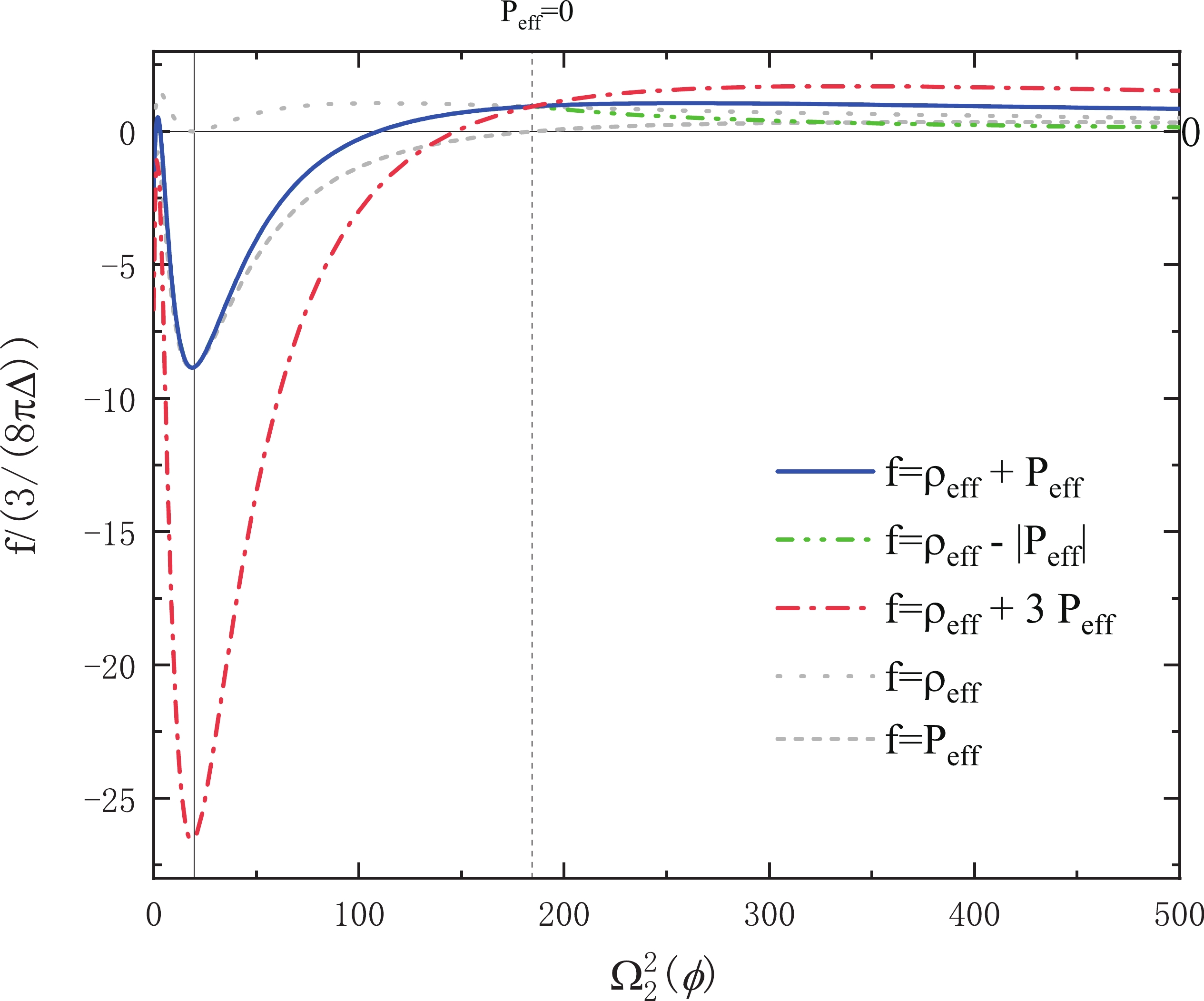
Figure 2. (color online) Behavior of
$ \rho_{\rm{eff}} $ ,$ P_{\rm{eff}} $ , and energy conditions for$ \gamma = 0.2375 $ and$1.000\leqslant \Omega_2^2(\phi)\leqslant 500.0.$ A similar calculation can be given for the strong energy condition (42). The first equation in Eqs. (42) requires
$ \begin{aligned}\rho_{\rm{eff}}+P_{\rm{eff}} =& \frac{3\rho_\phi}{8\pi G\gamma^2\Delta\rho_{\rm{c}}^{\rm{TR}}}\frac{\gamma^4\Omega_2^4(\phi) -6(1+\gamma^2)\gamma^2\Omega_2^2(\phi)+(1+2\gamma^2)} {2(1+\gamma^2)(1+\gamma^2\Omega_2^2(\phi))^2} \\ \geqslant & 0,\end{aligned} $

(45) which holds if
$ 3(1+\gamma^2)-\sqrt{9(1+\gamma^2)^2-(2\gamma^2+1)}\geqslant \gamma^2\Omega_2^2(\phi), $

(46) or
$ \gamma^2\Omega_2^2(\phi)\geqslant 3(1+\gamma^2)+\sqrt{9(1+\gamma^2)^2-(2\gamma^2+1)}. $

(47) For
$ \gamma = 0.2375 $ , we have the corresponding numerical solution$ \Omega_2^2(\phi)\leqslant 3.203 $ or$ \Omega_2^2(\phi)\geqslant 109.1 $ , while for$ \gamma = $ $ 0.2740 $ , we have$ \Omega_2^2(\phi)\leqslant 2.445 $ or$ \Omega_2^2(\phi)\geqslant 83.48 $ . The second equation in Eqs. (42) requires$ \begin{aligned}[b] \rho_{\rm{eff}}+3P_{\rm{eff}} =& -\frac{3}{8\pi G\gamma^2\Delta}\left(\frac{3\rho_\phi(1-\gamma^2\Omega_2^2(\phi))} {2\rho_{\rm{c}}^{\rm{TR}}(1+\gamma^2)(1+\gamma^2\Omega_2^2(\phi))}\right.\\ &\left.-\frac{\rho_\phi(3-7\gamma^2\Omega_2^2(\phi))}{\rho_{\rm{c}}^{\rm{TR}} (1+\gamma^2\Omega_2^2(\phi))^2}+\frac{2\gamma^2\Omega_2^2(\phi)}{ (1+\gamma^2\Omega_2^2(\phi))^2}\right)\geqslant 0, \end{aligned} $

(48) which can be solved for
$ \Omega_2^2(\phi) $ by a numerical method. For$ \gamma = 0.2375 $ , the above equation holds if$ \Omega_2^2(\phi)\geqslant 146.9 $ . For$ \gamma = 0.2740 $ , the above equation holds if$ \Omega_2^2(\phi)\geqslant 112.3 $ . Then, noting the solution of Eq. (45), we can conclude that the strong energy condition holds if$ \Omega_2^2(\phi)\geqslant 146.9 $ for$ \gamma = 0.2375 $ , or if$ \Omega_2^2(\phi)\geqslant 112.3 $ for$ \gamma = $ $ 0.2740 $ .Now, we are ready to have an overall look at the violation of dominant and strong energy conditions. Recall that the bounce occurs at the point
$ \Omega_2^2(\phi) = \dfrac{1+2\gamma^2}{\gamma^2} $ . It is easy to see that the dominant energy condition with respect to the effective stress-energy tensor in the new model of LQC is violated at the period$ 3.203\leqslant $ $ \Omega_2^2(\phi)\leqslant 109.1 $ (for$ \gamma = 0.2375 $ ) or$ 2.445\leqslant \Omega_2^2(\phi)\leqslant 83.48 $ (for$ \gamma = 0.2740 $ ) around the bounce point, while the strong energy condition is violated at the period$ \Omega_2^2(\phi)\leqslant 146.9 $ (for$ \gamma = 0.2375 $ ) or$ \Omega_2^2(\phi)\leqslant 112.3 $ (for$ \gamma = 0.2740 $ ). Hence, we can conclude that the strong energy condition is violated not only at a period around the bounce point, but also the whole period from the bounce point to the classical phase corresponding to the de Sitter epoch. All of these results for$ \gamma = 0.2375 $ are illustrated in Fig. 1 and Fig. 2. There are two branches of the evolution of the universe divided by the bounce point at$ \Omega_2^2(\phi) = \dfrac{1+2\gamma^2}{\gamma^2} = 6.210 $ for$ \gamma = 0.2375 $ . The effective pressure$ P_{\rm{eff}} $ is always negative in the branch that contains the de Sitter epoch, while it is negative only in a period near the bounce point in the other branch. -
The new model of LQC gives a remarkable prediction of the emergence of a de Sitter epoch [10, 11], in which the large cosmology constant from quantum geometry correction can influence the behavior of the energy conditions. We studied the interesting violation of energy condition problem in this model and considered the average null, dominant, and strong energy conditions with respect to the effective stress-energy tensor given by the effective dynamics equations. The results show that the quantum correction has a significant influence on the behaviors of the violation of energy conditions.
Based on the effective Hamiltonian constraint in the new model of LQC, we provided the effective dynamics equations and corresponding effective stress-energy tensor by comparing them with the standard Friedmann and Raychaudhuri equations. Then, the average null, dominant, and strong energy conditions with respect to the effective stress-energy tensor were expressed as functions of the physical time
$ \phi $ . The numerical calculation showed that, with respect to the effective stress-energy tensor in the new model of LQC, the average null energy condition is violated, while the dominant energy condition is violated only at a period around the bounce point. Last but not least, the strong energy condition is violated not only at a period around the bounce point, but also the whole period from the bounce point to the classical phase corresponding to the de Sitter period. Such a result is consistent with the appearance of the de Sitter epoch in the new model of LQC, in which the large effective cosmology constant is inversely proportional to the smallest non-zero area in LQG.In fact, the violation of the average null and strong energy conditions with respect to the effective stress-energy tensor has been approved in the standard LQC [15, 16], in which the strong energy condition is only violated near the bounce point compared with the new model of LQC. The new model of LQC introduces a de-Sitter epoch with a large effective cosmology constant coming from the loop quantum effects, which additionally contributes to the violation of energy conditions. However, the de-Sitter epoch is an asymptotic approximation in the large scale limit, and the period between the small and large scale is still difficult to describe in an intuitive formulation. Our study reveals the behaviors of the energy conditions with respect to the effective stress-energy tensor in the whole period of the evolution in this new model of LQC. More explicitly, we show that the strong energy condition is violated not only at a period around the bounce point, but also the whole period from the bounce point to the classical phase corresponding to the de Sitter epoch. This result indicates that the cosmology constant in our true universe may have a quantum gravity origin. Although the new model of LQC does not predict the correct cosmology constant, it still provides a new perspective for describing the origin of the cosmology constant, and it is expected to extend the core idea of this new model to other loop quantum gravity theories, i.e., loop quantum
$ f(R) $ theory and higher dimensional LQG [26-30], to find a proper quantum gravity theory that can predict the accurate cosmology constant in further research. Moreover, by sharing the same quantum geometry nature, our result is expected to be inherited in the full LQG, so that some light is shed on the construction of a wormhole and time machine, which usually require exotic matter to violate energy conditions.
Energy conditions in the new model of loop quantum cosmology
- Received Date: 2021-06-28
- Available Online: 2021-11-15
Abstract: Recently, a de-Sitter epoch has been found in the new model of loop quantum cosmology, which is governed by the scalar constraint with both Euclidean and Lorentz terms. The singularity free bounce in the new LQC model and the emergent cosmology constant strongly suggest that the effective stress-energy tensor induced by quantum corrections must violate the standard energy conditions. In this study, we perform an explicit calculation to analyze the behaviors of specific representative energy conditions, i.e., average null, strong, and dominant energy conditions. We reveal that the average null energy condition is violated at all times, while the dominant energy condition is violated only at a period around the bounce point. The strong energy condition is violated not only at a period around the bounce point but also in the whole period from the bounce point to the classical phase corresponding to the de Sitter period. Our results will shed some light on the construction of a wormhole and time machine, which usually require exotic matter to violate energy conditions.


 DownLoad: