


 Abstract
 HTML
HTML Reference
 Related
 PDF
PDF


-
Since it was first proposed in the 1920s, the existence of dark matter has been confirmed by many observations and experiments. In particular, the explanations of galaxy rotation curves [1, 2], gravitational lensing, and cosmic microwave background radiation have made dark matter widely accepted by many physicists. Researchers have thus paid more attention to dark matter research.
The neutrinos in the SM have hot dark matter characteristics, but the large scale structure of the universe supports the idea that cold dark matter is dominant. Therefore, the SM cannot provide a cold dark matter candidate. Although the SM has achieved great success with the detection of the 125 GeV Higgs boson, it has some shortcomings, such as the hierarchy problem, CP-violating problem, and neutrino with zero mass. Therefore, we consider extending the SM; the MSSM [3-5] is one choice of many supersymmetric models. However, the MSSM still fails to explain neutrino oscillation experiments, and its reasonable parameter space constrained by the experiments becomes increasingly smaller. Therefore, we need to expand the MSSM.
The BLMSSM [6-9] is an extension of the MSSM with local gauged B and L, whose local gauge group is
$ SU(3)_C\times SU(2)_L\times U(1)_Y \times U(1)_B\times U(1)_L $ and spontaneously broken at the TeV scale. The local gauged B can explain the asymmetry of matter-antimatter in the universe. At the same time, the local gauged L can improve the lepton flavor violating effect and give light neutrinos small mass with right handed neutrinos through the see-saw mechanism. The small hierarchy problem in the MSSM is relieved in the BLMSSM by exotic quarks and exotic leptons, which are introduced to eliminate the gauge anomalies. The BLMSSM can provide a new dark matter candidate beyond the MSSM. Therefore, we choose to use the BLMSSM to study dark matter.In current dark matter research, there are many dark matter candidates. They include massive compact halo objects (MACHOs) [10-12], primordial black holes, neutrinos, axions, and weakly-interacting massive particles (WIMPs) [13-17]. They all satisfy or partially satisfy the following conditions: no electric charge and no color charge, remaining stable, and possessing a long life [18, 19]. These characteristics could explain the observed large scale structure of the universe. Thus, cold dark matter is favored.
In the MSSM, the scalar neutrinos are only left-handed and interact with gauge bosons at tree level. This model cannot satisfy the constraints present from the relic density or direct detection experiments because of the large cross section. The introduced right-handed neutrinos are inactive and stable. The sneutrinos are electric and color neutral. If the lightest mass eigenstate of the sneutrino mass squared matrix is the lightest supersymmetric particle (LSP), and its dominant element is the right-handed sneutrino, it will be a good dark matter candidate. The reason is that it can easily satisfy the experimental restrictions from dark matter direct detection and give reasonable relic density. Eventually, the lightest scalar neutrino is adopted as a candidate for dark matter in this paper. There are other studies of sneutrino dark matter in extensions of the MSSM [20-27].
After this introduction, we show the main contents of the BLMSSM in section II. Sections III and IV are devoted to the equations of relic density and direct detection. We calculate the numerical results and find a reasonable parameter space in the BLMSSM in section V. The discussion and conclusion are provided in section VI.
-
The detection of the lightest CP-even Higgs at LHC [28-30] has proved that the SM can achieve great success. Extending the MSSM with the local gauge group
$ SU(3)_C\times SU(2)_L \times U(1)_Y\times U(1)_{B}\times U(1)_{L} $ , physicists have obtained the BLMSSM [6, 7]. Exotic leptons and exotic quarks are respectively introduced to cancel the L and B anomalies. The superfields in the BLMSSM are shown in Table 1. The Higgs superfields (two doublets and four singlets) obtain nonzero vacuum expectation values (VEVs). Therefore, they break both the lepton number and baryon number spontaneously.superfields $ SU(3)_C $ 

$ SU(2)_L $ 

$ U(1)_Y $ 

$ U(1)_B $ 

$ U(1)_L $ 

$ \hat{Q} $ 

3 2 1/6 1/3 0 $ \hat{U}^c $ 

$ \bar{3} $ 

1 −2/3 −1/3 0 $ \hat{D}^c $ 

$ \bar{3} $ 

1 1/3 −1/3 0 $ \hat{L} $ 

1 2 −1/2 0 1 $ \hat{E}^c $ 

1 1 1 0 −1 $ \hat{N}^c $ 

1 1 0 0 −1 $ \hat{Q}_4 $ 

3 2 1/6 $ B_4 $ 

0 $ \hat{U}_4^c $ 

$ \bar{3} $ 

1 −2/3 $- B_4 $ 

0 $ \hat{D}_4^c $ 

$ \bar{3} $ 

1 1/3 $- B_4 $ 

0 $ \hat{L}_4 $ 

1 2 −1/2 0 $ L_4 $ 

$ \hat{E}_4^c $ 

1 1 1 0 $- L_4 $ 

$ \hat{N}_4^c $ 

1 1 0 0 $ -L_4 $ 

$ \hat{Q}_5^c $ 

$ \bar{3} $ 

2 −1/6 $ -1-B_4 $ 

0 $ \hat{U}_5 $ 

3 1 2/3 $ 1+B_4 $ 

0 $ \hat{D}_5 $ 

3 1 −1/3 $ 1+B_4 $ 

0 $ \hat{L}_5^c $ 

1 2 1/2 0 $ -3-L_4 $ 

$ \hat{E}_5 $ 

1 1 −1 0 $3+ L_4 $ 

$ \hat{N}_5 $ 

1 1 0 0 $ 3+L_4 $ 

$ \hat{H}_u $ 

1 2 1/2 0 0 $ \hat{H}_d $ 

1 2 −1/2 0 0 $ \hat{\Phi}_B $ 

1 1 0 1 0 $ \hat{\varphi}_B $ 

1 1 0 −1 0 $ \hat{\Phi}_L $ 

1 1 0 0 −2 $ \hat{\varphi}_L $ 

1 1 0 0 2 $ \hat{X} $ 

1 1 0 $ 2/3+B_4 $ 

0 $ \hat{X}' $ 

1 1 0 $ -2/3-B_4 $ 

0 Table 1. Superfields in the BLMSSM.
After the Higgs obtain VEVs, the local gauge symmetry
$ SU(2)_{L}\otimes U(1)_{Y}\otimes U(1)_{B}\otimes U(1)_{L} $ breaks down to the electromagnetic symmetry$ U(1)_{e} $ . If we mark the nonzero VEVs of the$ SU(2)_L $ singlets$ \Phi_{B},\;\varphi_{B},\;\Phi_{L},\;\varphi_{L} $ and the$ SU(2)_L $ doublets$ H_{u},\;H_{d} $ as$ \upsilon_{{B}},\;\overline{\upsilon}_{{B}},\;\upsilon_{L},\;\overline{\upsilon}_{L},\;\upsilon_{u} $ , and$ \upsilon_{d} $ , we have$ \begin{aligned}[b] &H_{u} \!=\! \left(\!\!\!\!\!\begin{array}{c}H_{u}^+\\{\dfrac{1}{\sqrt{2}}}\Big(\upsilon_{u}\!+\!H_{u}^0\!+\!{\rm i}P_{u}^0\Big)\end{array}\!\!\!\!\!\right)\;,\; H_{d} \!=\! \left(\!\!\!\!\!\begin{array}{c}{\dfrac{1}{\sqrt{2}}}\Big(\upsilon_{d}\!+\!H_{d}^0\!+\!{\rm i}P_{d}^0\Big)\\H_{d}^-\end{array}\!\!\!\!\!\right)\;, \\ &\Phi_{B} = {1\over\sqrt{2}}\Big(\upsilon_{B}+\Phi_{B}^0+{\rm i}P_{B}^0\Big)\;,\;\; \varphi_{B} = {1\over\sqrt{2}}\Big(\overline{\upsilon}_{B}+\varphi_{B}^0+{\rm i}\overline{P}_{B}^0\Big)\;, \\ &\Phi_{L} = {1\over\sqrt{2}}\Big(\upsilon_{L}+\Phi_{L}^0+{\rm i}P_{L}^0\Big)\;,\;\;\varphi_{L} = {1\over\sqrt{2}}\Big(\overline{\upsilon}_{L}+\varphi_{L}^0+{\rm i}\overline{P}_{L}^0\Big)\;. \end{aligned} $

(1) The superpotential of the BLMSSM is [8]
$ \begin{aligned}[b] {\cal W}_{{\rm BLMSSM}} \!=& {\cal W}_{{\rm MSSM}}+{\cal W}_{B}+{\cal W}_{L}+{\cal W}_{X}\;, \\ {\cal W}_{B} \!=& \lambda_{Q}\hat{Q}_{4}\hat{Q}_{5}^c\hat{\Phi}_{B}+\lambda_{U}\hat{U}_{4}^c\hat{U}_{5} \hat{\varphi}_{B}+\lambda_{D}\hat{D}_{4}^c\hat{D}_{5}\hat{\varphi}_{B}\\ &+\mu_{B}\hat{\Phi}_{B}\hat{\varphi}_{B} +Y_{{u_4}}\hat{Q}_{4}\hat{H}_{u}\hat{U}_{4}^c+Y_{{d_4}}\hat{Q}_{4}\hat{H}_{d}\hat{D}_{4}^c \\ &+Y_{{u_5}}\hat{Q}_{5}^c\hat{H}_{d}\hat{U}_{5}+Y_{{d_5}}\hat{Q}_{5}^c\hat{H}_{u}\hat{D}_{5}\;, \\ {\cal W}_{L} \!=& Y_{{e_4}}\hat{L}_{4}\hat{H}_{d}\hat{E}_{4}^c+Y_{{\nu_4}}\hat{L}_{4}\hat{H}_{u}\hat{N}_{4}^c +Y_{{e_5}}\hat{L}_{5}^c\hat{H}_{u}\hat{E}_{5}\\ &+\!Y_{{\nu_5}}\hat{L}_{5}^c\hat{H}_{d}\hat{N}_{5} \!+\!Y_{\nu}\hat{L}\hat{H}_{u}\hat{N}^c\!+\!\lambda_{{N^c}}\hat{N}^c\hat{N}^c\hat{\varphi}_{L} \!+\!\mu_{L}\hat{\Phi}_{L}\hat{\varphi}_{L}, \\ {\cal W}_{X} \!=& \lambda_1\hat{Q}\hat{Q}_{5}^c\hat{X}+\lambda_2\hat{U}^c\hat{U}_{5}\hat{X}^\prime +\lambda_3\hat{D}^c\hat{D}_{5}\hat{X}^\prime+\mu_{X}\hat{X}\hat{X}^\prime\;, \end{aligned} $

(2) where
$ {\cal W}_{{\rm MSSM}} $ is the superpotential of the MSSM. The soft breaking terms$ {\cal L}_{{\rm soft}} $ of the BLMSSM can be written as [8].$ \begin{aligned}[b] {\cal L}_{{\rm soft}} =& {\cal L}_{{\rm soft}}^{\rm MSSM}-(m_{{\tilde{N}^c}}^2)_{{IJ}}\tilde{N}_I^{c*}\tilde{N}_J^c -m_{{\tilde{Q}_4}}^2\tilde{Q}_{4}^\dagger\tilde{Q}_{4}-m_{{\tilde{U}_4}}^2\tilde{U}_{4}^{c*}\tilde{U}_{4}^c \\ &-m_{{\tilde{D}_4}}^2\tilde{D}_{4}^{c*}\tilde{D}_{4}^c -m_{{\tilde{Q}_5}}^2\tilde{Q}_{5}^{c\dagger}\tilde{Q}_{5}^c-m_{{\tilde{U}_5}}^2\tilde{U}_{5}^*\tilde{U}_{5} -m_{{\tilde{D}_5}}^2\tilde{D}_{5}^*\tilde{D}_{5}\\ &-m_{{\tilde{L}_4}}^2\tilde{L}_{4}^\dagger\tilde{L}_{4}-m_{{\tilde{\nu}_4}}^2\tilde{N}_{4}^{c*}\tilde{N}_{4}^c -m_{{\tilde{e}_4}}^2\tilde{E}_{_4}^{c*}\tilde{E}_{4}^c-m_{{\tilde{L}_5}}^2\tilde{L}_{5}^{c\dagger}\tilde{L}_{5}^c \\ &-m_{{\tilde{\nu}_5}}^2\tilde{N}_{5}^*\tilde{N}_{5}-m_{{\tilde{e}_5}}^2\tilde{E}_{5}^*\tilde{E}_{5} -m_{{\Phi_{B}}}^2\Phi_{B}^*\Phi_{B} -m_{{\varphi_{B}}}^2\varphi_{B}^*\varphi_{B}\\ &-m_{{\Phi_{L}}}^2\Phi_{L}^*\Phi_{L} -m_{{\varphi_{L}}}^2\varphi_{L}^*\varphi_{L}-\Big(m_{B}\lambda_{B}\lambda_{B} +m_{L}\lambda_{L}\lambda_{L}+{\rm h.c.}\Big) \\ &+\Big\{A_{{u_4}}Y_{{u_4}}\tilde{Q}_{4}H_{u}\tilde{U}_{4}^c+A_{{d_4}}Y_{{d_4}}\tilde{Q}_{4}H_{d}\tilde{D}_{4}^c +A_{{u_5}}Y_{{u_5}}\tilde{Q}_{5}^cH_{d}\tilde{U}_{5} \\ &+A_{{d_5}}Y_{{d_5}}\tilde{Q}_{5}^cH_{u}\tilde{D}_{5}+A_{{BQ}}\lambda_{Q}\tilde{Q}_{4}\tilde{Q}_{5}^c\Phi_{B}+A_{{BU}}\lambda_{U}\tilde{U}_{4}^c\tilde{U}_{5}\varphi_{B} \\ &+A_{{BD}}\lambda_{D}\tilde{D}_{4}^c\tilde{D}_{5}\varphi_{B}+B_{B}\mu_{B}\Phi_{B}\varphi_{B} +{\rm h.c.}\Big\} \\ &+\Big\{A_{{e_4}}Y_{{e_4}}\tilde{L}_{4}H_{d}\tilde{E}_{4}^c+A_{{\nu_4}}Y_{{\nu_4}}\tilde{L}_{4}H_{u}\tilde{N}_{4}^c +A_{{e_5}}Y_{{e_5}}\tilde{L}_{5}^cH_{u}\tilde{E}_{5}\\ &+A_{{\nu_5}}Y_{{\nu_5}}\tilde{L}_{5}^cH_{d}\tilde{N}_{5} +A_{N}Y_{\nu}\tilde{L}H_{u}\tilde{N}^c+A_{{N^c}}\lambda_{{N^c}}\tilde{N}^c\tilde{N}^c\varphi_{L} \\ &+B_{L}\mu_{L}\Phi_{L}\varphi_{L}+{\rm h.c.}\Big\} +\Big\{A_1\lambda_1\tilde{Q}\tilde{Q}_{5}^cX+A_2\lambda_2\tilde{U}^c\tilde{U}_{5}X^\prime \\ &+A_3\lambda_3\tilde{D}^c\tilde{D}_{5}X^\prime+B_{X}\mu_{X}XX^\prime+{\rm h.c.}\Big\}\;. \end{aligned} $

(3) $ {\cal L}_{{\rm soft}}^{\rm MSSM} $ denote the soft breaking terms of the MSSM.The elements of the mass squared matrix of a sneutrino read as [ 9]
$ \begin{aligned}[b] M_{\tilde n}^2(\tilde\nu_I^* \tilde\nu_J) \!=& \frac{g_1^2+g_2^2}{8}(v_d^2-v_u^2)\delta_{IJ}+g_L^2(\bar{v}_L^2-v_L^2)\delta_{IJ}\\ &+\frac{v_u^2}{2}(Y_\nu^{\dagger} Y_\nu)_{IJ}+(m_{\tilde L}^2)_{IJ}, \\ M_{\tilde n}^2(\tilde N_I ^{c*} \tilde N _J ^c) \!=& -g_L^2(\bar{v}_L^2-v_L^2)\delta_{IJ}+\frac{v_u^2}{2}(Y_\nu^{\dagger} Y_\nu)_{IJ}+2\bar{v}_L^2({\lambda}_{N^c}^{\dagger} {\lambda}_{N^c})_{IJ} \\ &+(m_{\tilde N^c} ^2)_{IJ}+{\mu}_L\frac{v_L}{\sqrt 2}(\lambda_{N^c})_{IJ}-\frac{\bar v _L}{\sqrt 2}(A_{N^c})_{IJ}({\lambda}_{N^c})_{IJ}, \\ M_{\tilde n}^2(\tilde\nu_I \tilde N_J^c) \!= &{\mu}^* \frac{v_d}{\sqrt 2}(Y_\nu)_{IJ}\!-\!v_u \bar v_L(Y_\nu^{\dagger}\lambda_{N^c})_{IJ}\!+\!\frac{v_u}{\sqrt 2}(A_N)_{IJ}(Y_\nu)_{IJ}. \end{aligned} $

(4) The scalar neutrino mass squared matrix is diagonalized by the matrix
$ Z_{\tilde{\nu}} $ [31]. The lightest mass eigenstate of the scalar neutrino is considered to be dark matter in this work.With the introduced superfields
$ \hat{N}^c $ , three neutrinos obtain tiny masses through the see-saw mechanism. The mass matrix of neutrinos is shown in the basis$ (\psi_{\nu_L^I}, \psi_{N_R^{cI}}) $ ,$ \begin{aligned}[b] &Z_{N_{\nu}}^\top\left(\begin{array}{cc} 0&\dfrac{v_u}{\sqrt{2}}(Y_{\nu})^{IJ} \\ \dfrac{v_u}{\sqrt{2}}(Y^{T}_{\nu})^{IJ} & \dfrac{\bar{v}_L}{\sqrt{2}}(\lambda_{N^c})^{IJ} \end{array}\right)Z_{N_{\nu}} = {\rm diag}(m_{\nu^{\alpha}}), \\ &\alpha = 1\cdots 6,I,J = 1,2,3, \\ &\psi_{{\nu_L^I}} = Z_{{N_{\nu}}}^{I\alpha}k_{N_\alpha}^0,\;\;\;\; \psi_{N_R^{cI}} = Z_{{N_{\nu}}}^{(I+3)\alpha}k_{N_\alpha}^0,\;\;\;\; \chi_{N_\alpha}^0 = \left(\begin{array}{c} k_{N_\alpha}^0\\ \bar{k}_{N_\alpha}^0 \end{array}\right), \end{aligned} $

(5) where
$ \chi_{N_\alpha}^0 $ represents the mass eigenstates of neutrino fields.In the BLMSSM, the mass squared matrix of the slepton reads as
$ \left(\begin{array}{cc}({\cal M}^2_L)_{LL}&({\cal M}^2_L)_{LR}\\ ({\cal M}^2_L)^\dagger_{LR}&({\cal M}^2_L)_{RR}\end{array}\right). $

(6) $ {({\cal M}^2_L)}_{LL} $ ,$ {(\cal M}^2_L)_{LR} $ , and$ {({\cal M}^2_L)}_{RR} $ are shown here$ \begin{aligned}[b] ({\cal M}^2_L)_{LL} =& \frac{(g^2_1-g^2_2)(v^2_d-v^2_u)}{8} \delta_{IJ}+g^2_L(\bar{v}^2_L-v^2_L)\delta_{IJ}\\ &+{m^2_{l^I}}\delta_{IJ}+(m^2_{\bar{L}})_{IJ}, \\ ({\cal M}^2_L)_{LR} = &{\mu^\ast v_u\over\sqrt{2}}(Y_l)_{IJ}-{v_u\over\sqrt{2}}(A'_l)_{IJ}+{v_d\over\sqrt{2}}(A_l)_{IJ}, \\ ({\cal M}^2_L)_{RR} =&{g^2_1(v^2_u-v^2_d)\over4}\delta_{IJ}-g^2_L(\bar{v}^2_L-v^2_L)\delta_{IJ}+m^2_{l^I}\delta_{IJ}+(m^2_{\tilde{R}})_{IJ}. \end{aligned} $

(7) We rotate this mass squared matrix to the mass eigenstates through the unitary matrix
$ Z_{\tilde{L}} $ .Some couplings are shown here. The couplings of the W-lepton-neutrino and Z-neutrino-neutrino are different from those in the MSSM, and their concrete forms are
$ \begin{aligned}[b] &{\cal L}_{Wl\nu} = -\frac{e}{\sqrt{2}s_W}W_{\mu}^+\sum\limits_{I = 1}^3\sum\limits_{\alpha = 1}^6Z_{N_{\nu}}^{I\alpha*}\bar{\chi}_{N_{\alpha}}^0\gamma^{\mu}P_{\rm L}l^I+{\rm h.c.}, \\ &{\cal L}_{Z\nu\nu} = -\frac{e}{2s_Wc_W}Z_{\mu}\sum\limits_{I = 1}^3\sum\limits_{\alpha,\beta = 1}^6 Z_{N_{\nu}}^{I\alpha*}Z_{N_{\nu}}^{I\beta}\bar{\chi}_{N_{\alpha}}^0\gamma^{\mu}P_{\rm L}\chi_{N_{\beta}}^0+{\rm h.c.}, \end{aligned} $

(8) where
$ s_W(c_W) $ represents$ \sin\theta_W(\cos\theta_W) $ .$ \theta_W $ is the Weinberg angle.The Z-sneutrino-sneutrino coupling is deduced as
$ {\cal L}_{Z\tilde{\nu}\tilde{\nu}} = -\frac{e}{2s_Wc_W}Z_{\mu}\sum\limits_{I = 1}^3\sum\limits_{i,j = 1}^6Z_{\tilde{\nu}}^{Ii*}Z_{\tilde{\nu}}^{Ij}\tilde{\nu}^{i*}{\rm i}(\overrightarrow{\partial}^{\mu} -\overleftarrow{\partial}^{\mu})\tilde{\nu}^j. $

(9) We also obtain the chargino-lepton-sneutrino and neutralino-neutrino-sneutrino couplings
$ \begin{aligned}[b] {\cal L}_{\chi^{\pm}l\tilde{\nu}} =& -\sum\limits_{I = 1}^3\sum\limits_{i = 1}^6\sum\limits_{j = 1}^2\bar{\chi}^-_j \Big(Y_l^{I} Z_-^{2j*}Z_{\tilde{\nu}}^{Ii*}P_{\rm R}+ \Big[\frac{e}{s_W}Z_+^{1j}Z_{\tilde{\nu}}^{Ii*} \\ &+Y_\nu^{Ii}Z_+^{2j}Z_{\tilde{\nu}}^{(I+3)i*}\Big]P_{\rm L} \Big)l^I\tilde{\nu}^{i*}+{\rm h.c.}, \\ {\cal L}_{\chi^0 \nu\tilde{\nu}} =& \sum\limits_{I,J = 1}^3\sum\limits_{i = 1}^4\sum\limits_{\alpha,k = 1}^6\bar{\chi}^0_i \left(\frac{e}{\sqrt{2}s_Wc_W}(Z_N^{1i}s_W-Z_N^{2i}c_W)Z_{\tilde{\nu}}^{Ik*}Z_{N_{\nu}}^{I\alpha}\right.\\ &\left.+\frac{Y_\nu^{IJ}}{\sqrt{2}}Z_N^{4i}(Z_{N_{\nu}}^{I\alpha} Z_{\tilde{\nu}}^{(J+3)k*}+Z_{N_{\nu}}^{(I+3)\alpha} Z_{\tilde{\nu}}^{Jk*})\right)P_{\rm L}\chi^{0}_{N_\alpha}\tilde{\nu}^{k*}+{\rm h.c.}. \end{aligned} $

(10) Here,
$ Z_- $ and$ Z_+ $ are used to diagonalize the chargino mass matrix.The charged Higgs-lepton-neutrino couplings read as
$ \begin{aligned}[b] {\cal L}_{H^\pm L\nu} =& \sum\limits^3_{I,J = 1}\sum\limits^6_{\alpha = 1}G^\pm\bar{\rm e}^J(Y^{I}_l\cos\beta Z_{N_{\nu}}^{I\alpha}\delta_{IJ} P_{\rm L}\\ &-Y^{IJ\ast}_\nu\sin\beta Z_{N_{\nu}}^{(I+3) \alpha}P_{\rm R})\chi^0_{N_\alpha} \\ &-\sum\limits^3_{I,J = 1}\sum\limits^6_{\alpha = 1}H^\pm\bar{\rm e}^J(Y^{I}_l\sin\beta Z_{N_{\nu}}^{I\alpha}\delta_{IJ}P_{\rm L}\\ &+Y^{IJ\ast}_\nu\cos\beta Z_{N_{\nu}}^{(I+3)\alpha}P_{\rm R})\chi^0_{N_\alpha}+{\rm h.c.} \end{aligned} $

(11) The couplings of CP-even Higgs with sneutrinos are
$ \begin{aligned}[b] {\cal L}_{\tilde{\nu}\tilde{\nu}H^0} =& \sum\limits_{i,j = 1}^6\tilde{N}^{i*}\tilde{N}^{j}\Big(H^0[(N^u_M)_{ij}\sin\alpha+(N^d_M)_{ij}\cos\alpha] \\ &+h^0[(N^u_M)_{ij}\cos\alpha-(N^d_M)_{ij}\sin\alpha]\Big), \\ (N^u_M)_{ij} =& \sum\limits_{I = 1}^3\left(\frac{e^2}{4s_W^2c_W^2}v_u Z_{\tilde{\nu}}^{Ii*}Z_{\tilde{\nu}}^{Ij}-\sum\limits_{J = 1}^3v_u|Y_{\nu}^{IJ}|^2\delta_{ij} \right. \\ & \left.+\left(\lambda_{\nu_c}^*\bar{v}_L-\frac{A_N}{\sqrt{2}}\right)Z_{\tilde{\nu}}^{(I+3)i*}Z_{\tilde{\nu}}^{Ij}\right),\\ (N^d_M)_{ij} = &-\sum\limits_{I = 1}^3\frac{e^2}{4s_W^2c_W^2}v_d Z_{\tilde{\nu}}^{Ii*}Z_{\tilde{\nu}}^{Ij} -\sum\limits_{I,J = 1}^3\frac{\mu^*}{\sqrt{2}}Y_{\nu}^{IJ}Z_{\tilde{\nu}}^{(I+3)i*}Z_{\tilde{\nu}}^{Jj}. \end{aligned} $

(12) -
We consider the lightest sneutrino
$ (\tilde{\nu}_j) $ to be a dark matter candidate in this paper, and its main element is right-handed. Any dark matter candidate should satisfy the relic density constraint. Therefore, as the result of theoretical calculation approaches the actual observed value, the more reliable this theory becomes. The$ \tilde{\nu}_j $ number density$ n_{\tilde{\nu}_j} $ is given by the Boltzmann equation [2, 32-34]$ \frac{{\rm d} n_{\tilde{\nu}_j}}{{\rm d}t} \!=\! -3Hn_{\tilde{\nu}_j}\!-\!\langle\sigma v\rangle_{SA}(n^2_{\tilde{\nu}_j}\!-\!n^2_{\tilde{\nu}_j eq}) \!-\!\langle\sigma v\rangle_{CA}(n_{\tilde{\nu}_j}n_\phi\!-\!n_{\tilde{\nu}_j eq}n_{\phi eq}). $

(13) $ \tilde{\nu}_j $ can both self-annihilate and co-annihilate with another field of particle$ \phi $ . When the annihilation rate of$ \tilde\nu_{j} $ becomes roughly equal to the Hubble expansion rate, the species freeze out at the temperature$ T_{\rm F} $ ,$ \langle\sigma v\rangle_{SA}n_{\tilde{\nu}_j}+\langle\sigma v\rangle_{CA}n_{\phi}\sim H(T_{\rm F}). $

(14) If we suppose
$ M_{\phi}>M_{\tilde\nu_{j}} $ [35],$ n_\phi = \left(\frac{M_\phi}{M_{\tilde{\nu}_j}}\right)^{3/2}{\rm{exp}}[(M_{\tilde{\nu}_j}-M_\phi)/T]n_{\tilde{\nu}_j}. $

(15) Then, it becomes
$ \left[\langle\sigma v\rangle_{SA}+\langle\sigma v\rangle_{CA} \left(\frac{M_\phi}{M_{\tilde{\nu}_j}}\right)^{3/2}{\rm{exp}}[(M_{\tilde{\nu}_j}-M_\phi)/T]\right]n_{\tilde{\nu}_j}\sim H(T_{\rm F}). $

(16) We calculate the self-annihilation cross section
$ \sigma(\tilde{\nu}_j \tilde{\nu}_j^* \rightarrow $ anything) and co-annihilation cross section$ \sigma(\tilde{\nu}_j \phi \rightarrow $ anything) to study its annihilation rate$ \langle\sigma v\rangle_{SA} $ ($ \langle\sigma v\rangle_{CA} $ ) and its relic density$ \Omega_D $ in the thermal history of the universe. In the frame of the central mass system, the annihilation rate can be written as$ \sigma v = a+bv^2 $ [2, 34, 36, 37], where$ v $ represents the relative velocity of the two particles in their initial states. The thermally averaged cross section times velocity$ \langle \sigma_{\rm eff} v\rangle $ was extended by the Edsjö and Gondolo, including the co-annihilations [38, 39]$ \langle \sigma_{\rm eff} v\rangle(x) = \dfrac{\displaystyle\int_2^\infty K_1\left(\dfrac{a}{x}\right)\displaystyle\sum\nolimits_{i,j = 1}^N\lambda(a^2,b_i^2,b_j^2)g_ig_j\sigma_{ij}(a){\rm d}a}{4x\left(\displaystyle\sum\nolimits_{i = 1}^NK_2\left(\frac{b_i}{x}\right)b_i^2g_i\right)^2}, $

(17) with
$x = \dfrac{T}{M_{\tilde{\nu}_j}}, \; \lambda(a^2,\;b_i^2,\;b_j^2) = a^4+b_i^4+b_j^4-2(a^2b_i^2+ a^2b_j^2\;+ $ $ b_i^2b_j^2)$ ,$ a = \sqrt{s}/M_{\tilde{\nu}_j} $ , and$ b_i = m_i/M_{\tilde{\nu}_j} $ .$ g $ is the number of relativistic degrees of freedom with mass less than$ T_{\rm F} $ .$ \sigma_{ij} $ is the cross section for the annihilation reaction$ ij $ to any allowed final state, including two SM and/or Higgs particles. Then, one can calculate the relic density, whose value is$ \Omega_D h^2 = 0.1186\pm 0.0020 $ [40].Ignoring some of the lower contributions, the main self-annihilation processes are as follows:
$ \tilde{\nu}_j\!+\!\tilde{\nu}_j\!\rightarrow $ $ \! \{(W\!+\!W),\; (Z\!+\!Z), $ $ (h^0\!+\!h^0),\; (\bar{l}_i\!+\! l_i),\; (\bar{\nu}_i\!+\! \nu_i),\; (\bar{u}_i\!+\! u_i),\; (\bar{d}_i\!+\! d_i)\} $ , with$ i = 1, 2,$ $ 3 $ and$ h^0 $ representing the lightest CP-even Higgs boson. The self-annihilation processes are plotted in Figs. 1-5.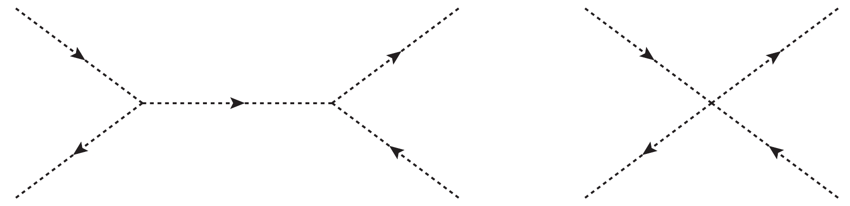
Figure 1. Feynman diagrams of
$ \tilde{\nu_j} \tilde{\nu_j} \rightarrow h^0 h^0. $ 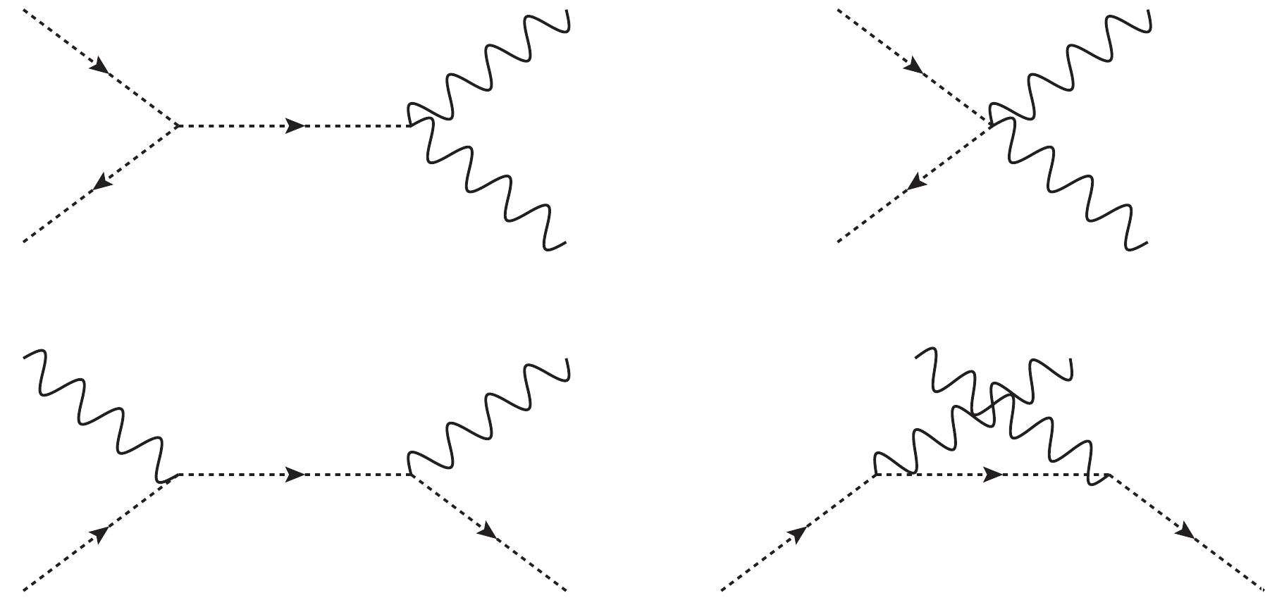
Figure 2. Feynman diagrams of
$\tilde \nu_j \tilde \nu_j \rightarrow ZZ.$ 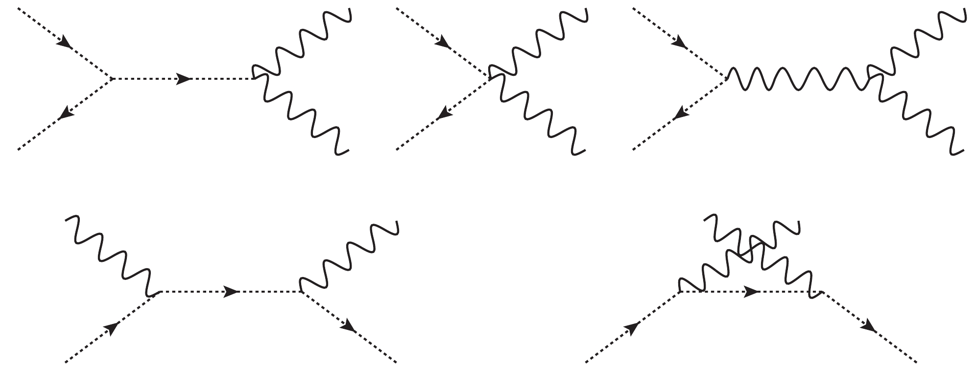
Figure 3. Feynman diagrams of
$\tilde \nu_j \tilde \nu_j \rightarrow WW.$ 
Figure 4. Feynman diagrams of
$\tilde \nu_j \tilde \nu_j \rightarrow \bar{\nu} \nu (\bar{l}l).$ 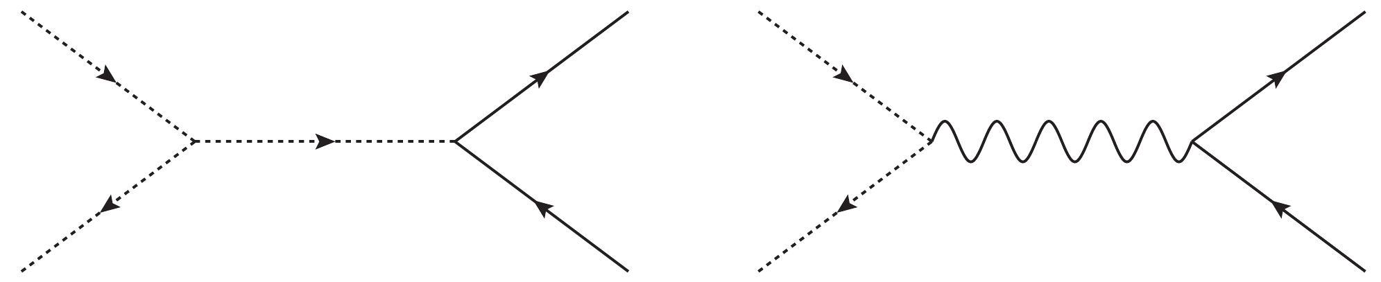
Figure 5. Feynman diagrams of
$ \tilde \nu_j \tilde \nu_j \rightarrow \bar{q}q. $ The studied co-annihilation processes read as [41]
a.
$\tilde{\nu}_j+\tilde{\nu}_k\rightarrow \{(W+W),\;\, (Z+Z),\; (h^0+h^0),\;\, (\bar{l}_i+ l_i)),\; \,(\bar{\nu}_i+ $ $ \nu_i),\;$ $(\bar{u}_i+ u_i),\; (\bar{d}_i+ d_i)\}$ with$k = 2\cdots 6,\; i = 1,\; 2,\; 3$ .b.
$ \tilde{\nu}_j+\chi^0_k\rightarrow \{(W^++l^-_i),\; (W^-+l^+_i),\; (Z+\nu_i)\} $ and$ k = $ $ 1\cdots 4, $ $ i = 1 \cdots 3 $ .c.
$ \;\tilde{\nu}_j+\chi^\pm_k\rightarrow \{(l^{\pm}_i+\gamma),\; (l^{\pm}_i+Z),\; (l^{\pm}_i+h^0),\; (W^{\pm}+\nu_i)\} $ and$ k = 1\cdots 2,\; i = 1\cdots 3 $ .d.
$ \tilde{\nu}_j+\tilde{L}^\pm_k\rightarrow \{(W^{\pm}_i+Z),\;\, (W^{\pm}_i+\gamma),\;\, (W^{\pm}_i+h^0),\;\, (\nu_i+l_i^\pm), $ $ (u_i+ \bar{d}_i),\; (d_i+\bar{u}_i)\} $ and$ k = 1\dots6,\; i = 1\dots3 $ .As examples, we show some results for the self-annihilation decays
$ \tilde \nu_j \tilde \nu_j\rightarrow h^0 h^0 $ and$ \tilde \nu_j \tilde \nu_j\rightarrow \bar{t}t $ . The Feynman diagrams for the process$ \tilde \nu_j \tilde \nu_j\rightarrow h^0 h^0 $ are plotted in Fig. 1. The lightest mass eigenstate of the CP-even Higgs$ H^0_i (i = 1,\; 2) $ is$ H_1^0 $ , represented by$ h^0 $ . The analytic results are deduced here.$ \begin{aligned}[b] \langle{\sigma v}\rangle_{h^0 h^0} =& \frac{|M|^2}{64\pi M_{\tilde {\nu}_j}^2}\sqrt{1-\frac{m_{h^0}^2}{M_{\tilde {\nu}_j}^2}},\\ {|M|}^2 =& {|{\cal D}|}^2+{\sum\limits_{i,k = 1}^2\frac{{\cal B}_i {\cal B}_k^* {\cal C}_i {\cal C}_k^*}{(M_{\tilde {\nu}_j}^2-m_{H_i^0}^2) (M_{\tilde {\nu}_j}^2-m_{H_k^0}^2)}}\\ &+2\Re\left[\sum\limits_{i = 1}^2\frac{{\cal D}^* {\cal B}_i{\cal C}_i}{(M_{\tilde {\nu}_j}^2 -m_{H_i^0}^2)}\right]. \end{aligned} $

(18) with
$ \begin{aligned}[b] &{\cal B}_i = -\frac {e^2({A_R^{11} B_R^i +2A_R^{1i} B_R^1})}{4s_W^2 c_W^2},\quad {\cal C}_i = -\sum\limits_1^3\frac{e^2 B_R^i{Z_{I1} {Z_{I1}^*}}}{4{s_W}^2 {c_W}^2}, \end{aligned} $

$ \begin{aligned}[b] &{\cal D} = -\frac{e^2 A_R^{11}}{4s_W^2 c_W^2} \sum\limits_{I = 1}^3{Z_{I1} Z_{I1}^*},\\& B_R^i = v_1 Z^{1i}_R-v_2 Z^{2i}_R,\\ &A_R^{ij} = Z_R^{1i} Z_R^{1j}-Z_R^{2i} Z_R^{2j}. \end{aligned} $

(19) $ Z_R $ is the matrix to diagonalize the mass squared matrix of the CP-even Higgs.The
$ \langle{\sigma v}\rangle $ for the process$ \tilde \nu_j \tilde \nu_j\rightarrow \bar{t}t $ is also shown here. This is the leading order contribution from the virtual CP-even Higgs. The virtual Z boson contribution is suppressed by the square of the relative velocity, and we do not show it here.$ \langle{\sigma v}\rangle_{\bar t t} = \frac{3(M_{\tilde \nu_j}^2-{m_t^2})}{32 \pi M_{\tilde \nu_j}^2} \frac{m^2_t}{v_u^2 }\sum\limits_{i,k = 1}^2\frac{8 {\cal C}_i {\cal C}_k^*}{(4M_{\tilde \nu_j}^2-m_{H_i^0}^2)(4M_{\tilde \nu_j}^2-{m_{H_k^0}^2})}. $

(20) -
At the quark level, the process for direct detection is
$ \tilde{\nu}+q\rightarrow \tilde{\nu}+q $ . The lightest sneutrino is predominantly composed of the right-handed sneutrino, which is not active. Thus, it can easily satisfy the constraint from the direct detection experiments. This special condition is represented by the neutrino Yukawa coupling in the mass squared matrix of the sneutrino. It leads to the suppression factor$ Z^{Ij}_{\nu}, \; I = (I = 1,2,3) $ appearing in the Feynman rules for the coupling$ Z-\tilde{\nu}-\tilde{\nu} $ and$ H^0(A^0)-\tilde{\nu}-\tilde{\nu} $ . The lightest sneutrino is represented by$ \tilde{\nu}_j $ and$ j>3 $ , with the right-handed sneutrinos labeled 4, 5, and 6. Then,$ Z^{Ij}_{\nu} $ is in direct proportion to the tiny neutrino Yukawa coupling$ Y_\nu $ . The order of$ Y_\nu $ is in the region of$ (10^{-6}\sim10^{-9}) $ .The cross section from virtual Z boson contribution is suppressed by
$ Y_\nu^4 $ , while the cross section of the process with the virtual CP-odd Higgs boson is suppressed by$ Y_\nu^2 v^4 $ , with$ v^4 $ coming from$ |\bar{q}\gamma_5 q|^2 $ [42]. The CP-even Higgs contribution is dominant, with the factor$ Y_\nu^2 $ . Therefore, the cross section for sneutrino scattering off a nucleon is at least suppressed by$ Y_\nu^2 $ . The large term is from the operator$ \tilde{\nu}^{*}\tilde{\nu}\bar{q}q $ at quark level. We should convert the quark level coupling to the effective nucleon coupling with the equations [ 42]$ \begin{aligned} &a_qm_q\bar{q}q\rightarrow f_Nm_N\bar{N}N,\quad f_N = \sum\limits_{q = u,d,s}f_{Tq}^{(N)}a_q+\frac{2}{27}f_{TG}^{(N)}\sum\limits_{q = c,b,t}a_q,\\ &\langle N|m_q \bar{q}q|N\rangle = m_N f_{Tq}^{(N)},\quad f_{TG}^{(N)} = 1-\sum\limits_{q = u,d,s}f_{Tq}^{(N)}. \end{aligned} $

(21) The numbers of
$ f_{Tq}^{(N)} $ are [43-45],$ \begin{aligned}[b] &f^{(p)}_{Tu} = 0.0153,\; \; \; f^{(p)}_{Td} = 0.0191,\; \; \; f^{(p)}_{Ts} = 0.0447, \\ &f^{(n)}_{Tu} = 0.0110,\; \; \; f^{(n)}_{Td} = 0.0273,\; \; \; f^{(n)}_{Ts} = 0.0447. \end{aligned} $

(22) With the obtained
$ f_N $ , the following scattering cross section is obtained:$ \sigma = \frac{1}{\pi}\mu_K^2[Z_pf_p+(A-Z_p)f_n]^2. $

(23) Here,
$ \mu_K $ is the effective mass of the nucleon-sneutrino system,$ Z_p $ is the proton number, and$ A $ represents the atomic number. -
To confine the used parameter, we take into account the experiment results from the Particle Data Group (PDG) [40]. The results from our previous works are also considered [41]. The mass of the lightest neutral CP-even Higgs
$ h^0 $ is$ m_{h^0} $ = 125.1 GeV [28, 29] in this work.The parameters used are listed in the following:
$ \begin{aligned}[b] &\tan\beta = 2,\; m_a = 1\;{\rm{TeV}}, \; AN_{11} = AN_{22} = -450\;{\rm{GeV}},\\ &AN_{33} \!=\! -40\;{\rm{GeV}}, V_L \!=\! 3\;{\rm{TeV}},\; \tan\beta_L\! =\! 2,\; \lambda_{11} \!=\! \lambda_{22} \!=\! 1,\;\\ &\lambda_{33} = -0.1,\; M_1 = M_2 = 1\;{\rm{TeV}}, \; \mu = 0.8\;{\rm{TeV}},\; g_L = \frac{1}{6},\;\\ &ML_{11} = ML_{22} = ML_{33} = 1\;{\rm{TeV}}^2,\; \mu_L = 0.5\;{\rm{TeV}}. \end{aligned} $

(24) In addition to the fixed parameters shown above, there are some adjustable parameters, defined as
$ \tau_{ii} = \left(M^2_{\tilde{E}}\right)_{ii},\; \; \rho_{ii} = \left(M^2_{\tilde{\nu}}\right)_{ii},\; \; \xi_{ii} = AL_{ii},\; \; \epsilon_{ii} = AL^\prime_{ii},\; (i = 1,\; 2,\; 3). $

(25) When we set these values as
$ \tau_{ii} = 25.2\;{\rm{TeV}}^2,\; \rho_{ii} = $ $ 0.1\;{\rm{TeV}}^2, \; \xi_{ii} = 14\;{\rm{TeV}},\; \epsilon_{ii} = 3\;{\rm{TeV}}, $ and all the off-diagonal elements of the matrixes$ ((M^2_{\tilde{E}})_{ij}, (M^2_{\tilde{\nu}})_{ij},AL_{ij},AL^\prime_{ij} $ with$ i\neq j) $ are zero, the numerical result for the dark matter relic density is$ \Omega_D h^2 $ = 0.118581. This is very close to the experimental central value and within one$ \sigma $ sensitivity.At this point, the lightest scalar neutrino mass is 350 GeV, and the other scalar neutrinos' masses are all larger than 1 TeV. Additionally, the lightest scalar lepton mass is approximately 1073 GeV, and the masses of heavier scalar leptons are on the order of several TeV. The heavy CP-even Higgs mass is approximately 1 TeV. The masses of neutralinos are in the region of
$ 768\sim1033 \;{\rm{GeV}}$ . The two mass eigenstates of charginos are 1021 and 781 GeV. Therefore, the lightest scalar neutrino is indeed the LSP in this condition. Considering the masses of the above particles, the resonance effect cannot take place because the exchanged particle in the S channel is not near$ 2\times350 = 700 \;{\rm{GeV}}$ .We next study how these variables affect the results.
$ \tau_{ii} $ are the diagonal elements in the scalar lepton mass squared matrix, which can influence the scalar lepton masses. Similarly,$ \rho_{ii} $ are the diagonal elements of the scalar neutrino mass squared matrix. The non-diagonal elements of the scalar lepton mass squared matrix include the parameters$ \xi_{ii} $ and$ \epsilon_{ii} $ . In the whole,$ \tau_{ii} $ ,$ \rho_{ii} $ ,$ \xi_{ii} $ , and$ \epsilon_{ii} $ give effects to the scalar leptons (scalar neutrinos) masses and mixing. Therefore, the relic density is influenced by these parameters.In Fig. 6, we keep the parameters
$ \rho_{ii} = 0.1\;{\rm{TeV}}^2, $ $ \xi_{ii} = 14\;{\rm{TeV}},\; \epsilon_{ii} = 3\;{\rm{TeV}}, $ and plot the results of$ \Omega_D h^2 $ with$ \tau_{ii} $ . The$ \Omega_D h^2 $ is a weakly increasing function, as$ \tau_{ii} $ is on the specified interval from 23 to 27 TeV2. When$ \tau_{ii} $ varies from 24.6 to 25.8 TeV2, the$ \Omega_D h^2 $ is in the band of$ 3 \sigma $ sensitivity, denoted by the gray area in Fig. 6. From these data, we can see that the masses of various particles are below a few TeV, which is consistent with the constraints from the LHC. Therefore, we believe that our results may be verified experimentally before long. Because the energy range of the particles is fairly wide, it is more advantageous to test them experimentally in the future.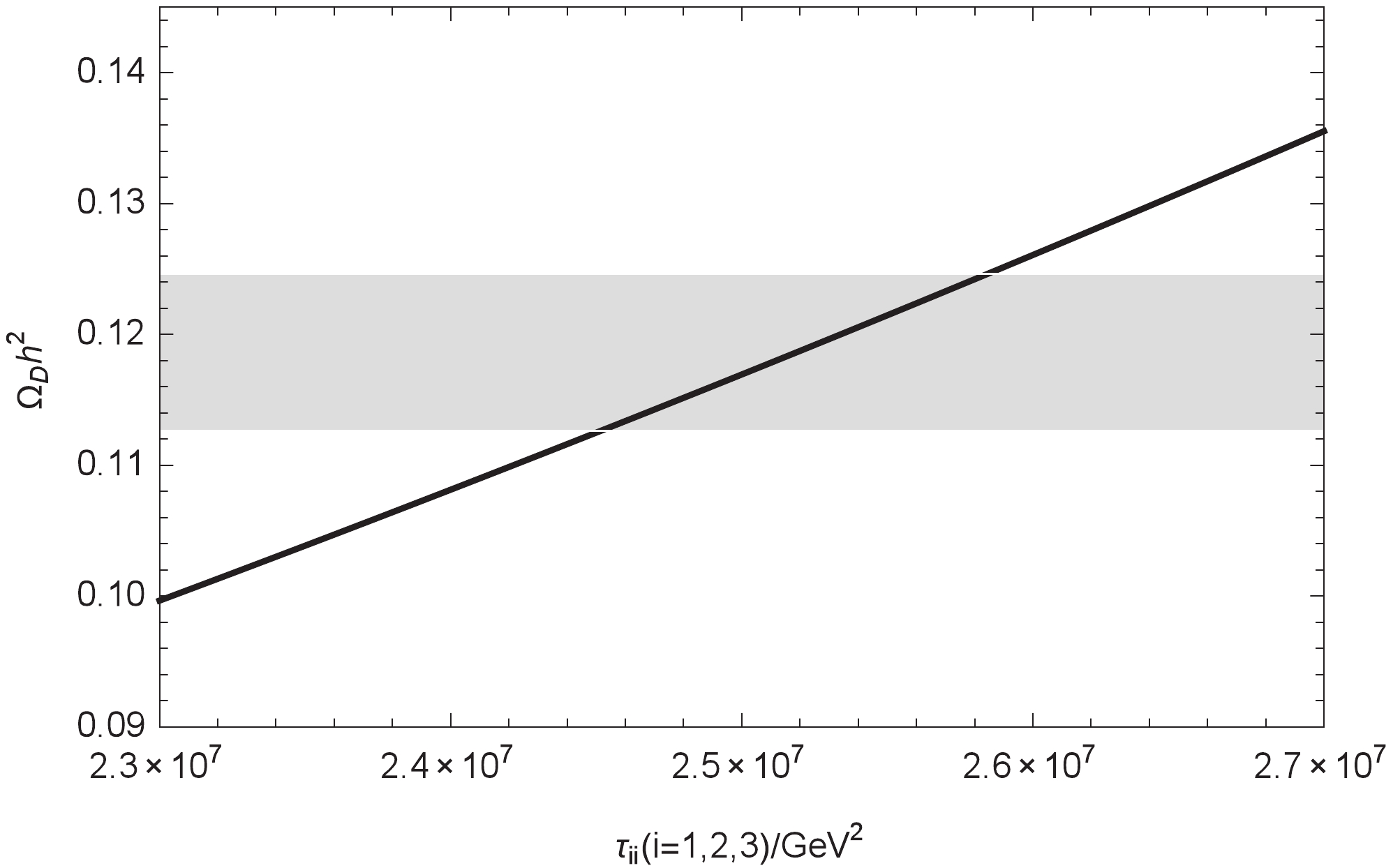
Figure 6. Relationship between
$ \Omega_D h^2 $ and$\tau_{ii}.$ On the contrary, Fig. 7 shows that
$ \Omega_D h^2 $ is a decreasing function of$ \rho_{ii} $ within the selected interval (95000~107000) GeV2. The value of$ \Omega_D h^2 $ decreases rapidly as the value of$ \rho_{ii} $ increases. The reason for this is that as$ \rho_{ii} $ increases, heavier scalar neutrino masses are obtained. At the same time, the matrix to diagonalize the scalar neutrino mass matrix changes, which influences the results directly and obviously. When$ \rho_{ii} $ is in the range of approximately$ 9.85\times10^4 $ to$ 1.01\times10^5 \;{\rm{GeV^2}} $ , we can ensure that$ \Omega_D h^2 $ is within a reasonable range of$ 3 \sigma $ .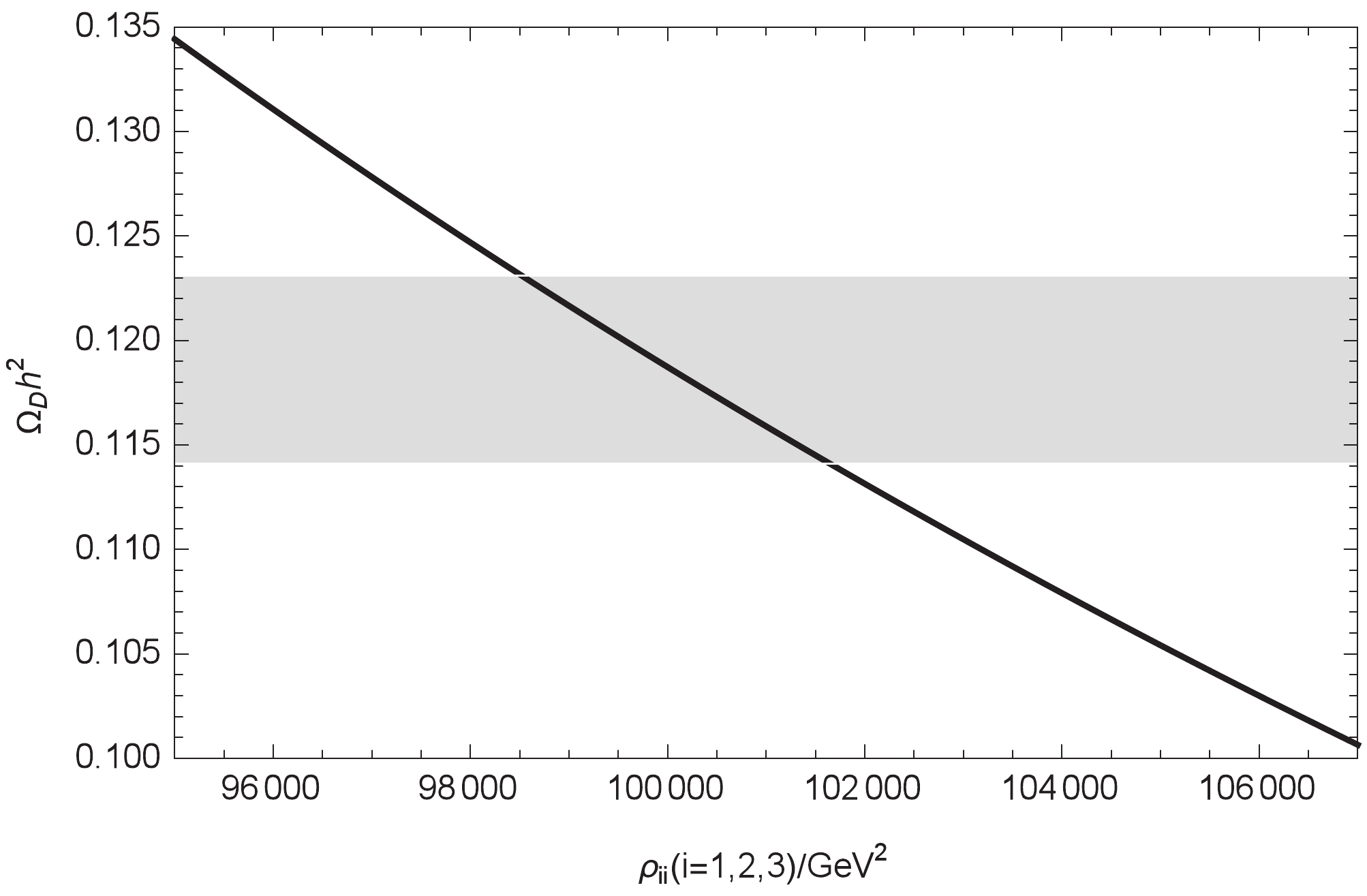
Figure 7. Relationship between
$ \Omega_D h^2 $ and$\rho_{ii}.$ The relationship of
$ \Omega_D h^2 $ with$ \xi_{ii} $ and$ \epsilon_{ii} $ is a little bit more interesting. In Fig. 8 and Fig. 9, the values of$ \Omega_D h^2 $ are almost quadratic functions of the variables$ \xi_{ii} $ and$ \epsilon_{ii} $ , respectively. As$ \xi_{ii} $ is in the range of -25 to 35 TeV, the values of$ \Omega_D h^2 $ are all acceptable. The behavior of$ \Omega_D h^2 $ versus$ \epsilon_{ii} $ in Fig. 9 is similar to the condition in Fig. 8. To satisfy the experimental constraint, the region where$ \epsilon_{ii} $ varies from -6 to 5 TeV is acceptable. From Fig. 8 and Fig. 9, we can obtain the best values for$ \xi_{ii} = 14\;{\rm{TeV}} $ and$ \epsilon_{ii} = 3\;{\rm{TeV}} $ .
Figure 8. Relationship between
$ \Omega_D h^2 $ and$\xi_{ii}.$ 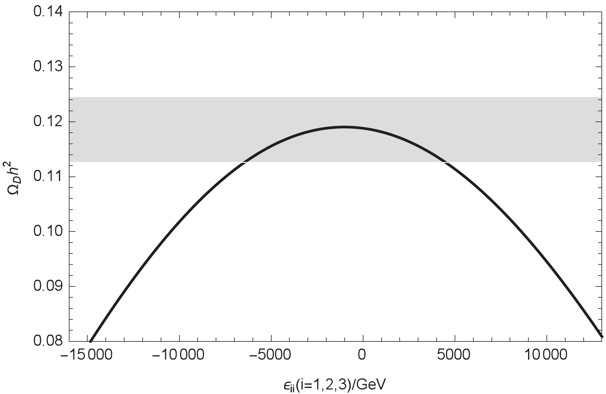
Figure 9. Relationship between
$ \Omega_D h^2 $ and$\epsilon_{ii}.$ With the parameters satisfying the relic density, which is shown in the first part of this section, we study the spin-independent cross section
$ \sigma^{SI} $ for sneutrino scattering off a nucleon versus$ \epsilon_{ii} $ in Fig. 10.$ \sigma^{SI} $ increases slightly with increasing$ \epsilon_{ii} $ from$ 9\times10^4 $ to$ 12\times10^4 $ GeV2. The corresponding theoretical value of$ \sigma^{SI} $ is in the region of$ (7.8\sim8.05)\times 10^{-48} \; {\rm{cm}}^2 $ . The lightest sneutrino mass is approximately 350 GeV, whose constraint from the direct detection experiments of$ \sigma^{SI} $ is approximately$ 3.0 \times 10^{-46}{\rm{cm}}^2 $ [46, 47]. Our numerical results for the spin-independent cross section are approximately two orders smaller than the experimental constraint.
Figure 10. Relationship between the spin-independent cross section and
$\epsilon_{ii}.$ In Fig. 11, we plot
$ \sigma^{SI} $ versus$ A_n = AN_{11} = AN_{22} $ .$ A_n $ is the parameter in the non-diagonal element of the mass matrix and multiplies neutrino Yukawa coupling. Therefore, it can have a considerable effect on the cross section of direct detection. As$ A_n $ varies from -1500 to 1500 GeV,$ \sigma^{SI} $ decreases from$ 1.2\times10^{-47} $ to$ 2.0\times10^{-48} \; {\rm{cm}}^2 $ . On the whole, it can satisfy the constraints from the direct detection experiments.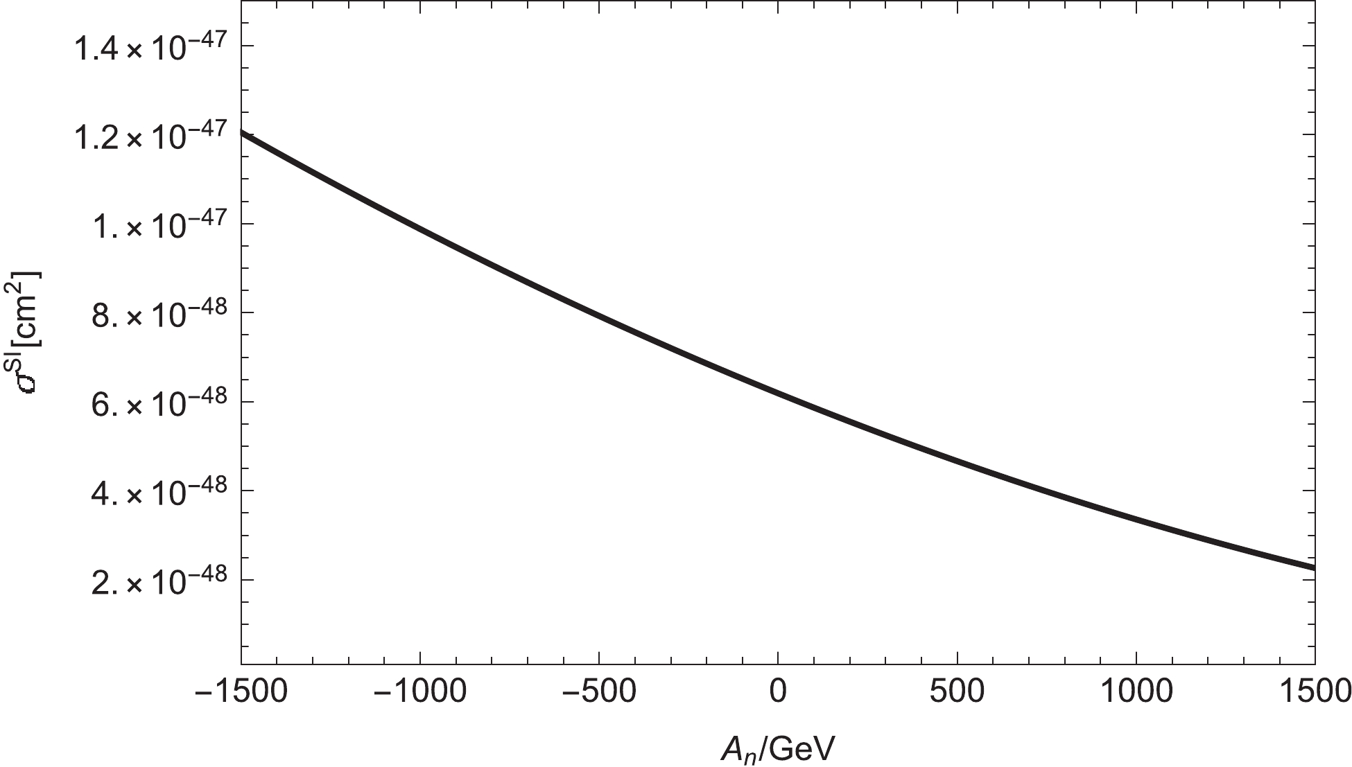
Figure 11. Relationship between the spin-independent cross section and
$A_{n}.$ -
The BLMSSM is an extension of the MSSM, wherein right-handed neutrinos, exotic Higgs singlets, exotic quarks, and exotic leptons are added to the MSSM. Through the seesaw mechanism, three light neutrinos obtain small masses, smaller than eV order. As we all know, the value of
$ \Omega_D h^2 $ is related to many parameters, such as$ \tau_{ii} $ ,$ \rho_{ii} $ , and$ \mu_L $ . Generally speaking, the parameters related to the cross section of scalar neutrino annihilation can affect the results to some extent. We find a reasonable parameter space to satisfy the relic density and direct detection experiments. Under these conditions, the lightest scalar neutrino mass is approximately 350 GeV as the LSP in the BLMSSM.Currently, theoretical physicists have proposed many models for dark matter, and the types of dark matter candidates are also enriched. In spite of this, the possibility space of reality is still much larger than our imagination. In our study, the lightest scalar neutrino could be a dark matter candidate in a reasonable range. In fact, it is one of several possibilities. Finally, we sincerely hope that researchers can uncover the real veil of dark matter as soon as possible through the full cooperation of physicists at home and abroad.
-
We are very grateful to Dr. Jing-Jing Feng of Beijing Normal University for solving some problems.
Scalar neutrino dark matter in the BLMSSM
- Received Date: 2021-04-19
- Available Online: 2021-09-15
Abstract: The BLMSSM is an extension of the minimal supersymmetric standard model (MSSM). Its local gauge group is


 DownLoad: