


 Abstract
 HTML
HTML Reference
 Related
 PDF
PDF


-
In recent years, a large number of new hadronic states containing heavy quarks (charm quark c or bottom quark b) have been observed in hadron and
$ e^+e^- $ colliders [1]. For example, the tetraquark states, pentaquark states, and baryons, which contain two heavy quarks [2-4]. These findings have opened up a new stage for the study of hadron physics and QCD. It is well known that the light flavor baryons are composed of three light quarks ($ u, d, s $ ), and all kinds of light flavor baryons from$ \Delta^{++}(uuu) $ to$ \Omega^- (sss) $ have been observed for many decades. For the heavy baryons, the singly charmed and bottom baryons (containing one heavy quark c or b and two light quarks) have already formed a subfamily within heavy hadrons in recent years. Remarkably, the doubly charmed baryon,$ \Xi^{++}_{cc}(ccu) $ , which contains two charm quarks and one light quark, was discovered in 2017 [5], and more of its kind are expected to be found soon. The discovery of the doubly charmed baryon is an important event, and it may indicate that the whole family of baryons with all flavors$ (u,d,s,c,b) $ may be found in the not far future. Here, the last member of the baryon family, i.e., the triply heavy baryons, which are composed of three heavy quarks c or b, are yet to be discovered.The
$ \Omega_{QQQ} $ baryons are made of three identical heavy quarks ($ Q = c, b $ ). Because of their special properties in the baryon family, the$ \Omega_{QQQ} $ baryons have been studied extensively for their productions [6-12], weak decays [13-15], masses [16-43] and so on. Particularly, the masses of$ \Omega_{QQQ} $ baryons have been evaluated using various approaches, including lattice QCD [16-22], QCD sum rules [23-25], potential models [26-37], the Fadeev equation [38-41], and the Regge trajectories [42, 43]. The predicted values for the masses of$ \Omega_{QQQ} $ baryons are listed in Table 5. As shown, the predicted masses are in a wide range, and different approaches produce different results. Therefore, it is still necessary to examine the$ \Omega_{QQQ} $ baryons.Models $\Omega_{ccc}/{\rm GeV}$ 

$\Omega_{bbb}/{\rm GeV}$ 

Lattic QCD [16-22] 4.7~4.8 14.36~14.37 QCD Sum Rules [23-25] 4.6~5.0 13.28~14.83 Various potential models [14, 26-37] 4.76~4.90 14.27~14.83 Fadeev equation [38-41] 4.76~5.00 14.23~14.57 Regge trajectories [42, 43] 4.834 14.788 This work $4.53^{+0.26}_{-0.11}$ 

4.75~4.80 GeV*$14.27^{+0.33}_{-0.32}$ 

In this paper, we present the study of
$ \Omega_{QQQ} $ baryon using the QCD sum rule [44-46] approach, which is known to be a powerful tool to evaluate hadron properties [47-50]. In this approach, one starts at short distances and then moves to long distances using the operator product expansion (OPE) for a given quark current's correlation function in QCD. The first term in the OPE is the dimensionless (d = 0) identity operator, which represents the perturbative QCD part, and then, as power corrections, the higher dimensional operators (d = 4, 6,$\cdots $ ) with vacuum condensations emerge, which represent the nonperturbative (confinement) contribution. Principally, because of the power suppression$\left(\dfrac{\Lambda _{\rm QCD}^2}{-q^2}\ll 1 \right)$ at small distances (large$ (-q^2) $ ), the high dimensional operator contributions should decrease as the power increases; one may only need to consider a few important terms in the OPE. Moreover, for the first (Identity) term in the OPE, i.e., the perturbative QCD term, one needs to consider not only the leading-order (LO) but also, at least, the next-to-leading order (NLO)$ O(\alpha_s) $ contributions ($ \alpha_s $ being the strong coupling constant), because the latter may lead to substantial corrections. Additionally, the$ O(\alpha_s) $ corrections to the coefficients of the power-suppressed condensation terms may also need to be considered. Practically, for the heavy$ \Omega_{QQQ} $ system, the most important contributions in the OPE are the perturbative term$ C_1 $ and gluon condensation term$ C_{GG} \langle g_s^2 \hat{G}\hat{G} \rangle $ , where$ C_1 $ and$ C_{GG} $ can be calculated perturbatively. As a good approximation, it may be necessary to consider the LO of$ C_1 $ , which is the most important contribution, the NLO of$ C_1 $ , which gives large corrections, and the LO of$ C_{GG} $ , which is the same order of magnitude as the former, but neglects other contributions. In fact, the importance of including the NLO contribution of$ C_1 $ has been emphasized in many studies, e.g., for the proton (uud) [51, 52], the singly heavy baryon [53], and the doubly heavy baryon$ \Xi_{cc}^{++} $ [54]. Our previous work [54] analyzed the NLO effect thoroughly for the doubly heavy baryon$ \Xi_{cc}^{++} $ and determined that the NLO correction is sizable for$ \Xi_{cc}^{++} $ and cannot be ignored in QCD sum rules. Accordingly, we expect that the NLO correction also produces a sizable contribution to triply heavy baryons (QQQ). Presently, no work has been conducted at the NLO level for triply heavy baryons. However, for some leading order (LO) results of the$ \Omega_{QQQ} $ [23-25], there are significant differences among different studies, as shown in the preceding paragraph. To reduce the uncertainties at the LO, it may be necessary to perform the NLO calculations in QCD sum rules. With the inclusion of the NLO contribution, the result should be substantially improved. Moreover, it is worthwhile to emphasize that there are significant differences between the fully heavy baryons and other baryons that contain light quarks. For the former, the most important nonperturbative contribution comes from the gluon condensation$ \left \langle GG \right \rangle $ , whereas for the latter, the light quark condensation$ \left \langle \bar{q}q \right \rangle $ makes the important contribution. This point will be embodied in our calculation for$ \Omega_{QQQ} $ in the QCD sum rules.The rest of the paper is organized as follows. In Sec. II, the sum rules for the calculation of the mass of
$ \Omega_{QQQ} $ are presented. In Sec. III, we introduce the methods and procedures for the calculation of the coefficients$ C_1 $ and$ C_{GG} $ . The phenomenology results and discussions are presented in Sec. IV. -
For the S-wave triply heavy quark
$ (QQQ) $ system, owing to Fermi-Dirac statistics [25, 55], there only exists the$ J^P = \dfrac{3}{2}^+ $ baryon ground state$ \Omega_{QQQ} $ ($ Q = c,\,b $ ), with the corresponding current$ J_{\mu} $ [23, 25, 55],$ J_{\mu} = \epsilon^{abc}(Q^T_a \hat{C}\gamma^\mu Q_b)\, Q_c\,, $

(1) where a, b, and c denote the color indices, and
$ \hat{C} $ is the charge-conjugation matrix. Because there is no QQQ ground state with$ J = \dfrac{1}{2} $ , it is not necessary to worry about the pollution from the$ J = \dfrac{1}{2} $ state in the analysis.In the QCD sum rules, we begin with the two-point correlation function
$ \Pi_{\mu \nu}(q^2) = {\rm i} \int {{\rm d}^4 x {\rm e}^{{\rm i}q \cdot x} \langle \Omega|T[J_\mu (x) \bar{J}_\nu(0)] |\Omega\rangle}, $

(2) where Ω represents the QCD vacuum. According to the Lorentz covariance, the matrix element of the current can be written as
$ \langle \Omega|J_{\mu}(0) |H(q,s)\rangle = \sqrt{\lambda} U_\mu(q,s), $

(3) where
$ H(q,s) $ denotes the ground state baryon with mass$ M_H $ , momentum q, and spin s; λ is the pole residue for H; and$ U_\mu(q,s) $ is the corresponding Rarita-Schwinger spinor, which satisfies the relation$ \begin{aligned}[b]\sum\limits_s U_\mu(q,s)\bar{U}_\nu(q,s) =\;& ({\not\!\!{q}} +M_H)\Biggr(-g_{\mu \nu} +\frac{\gamma_\mu \gamma_\nu}{3} \\ &\left.+ \frac{2 q_\mu q_\nu}{3 M_H^2}-\frac{q_\mu \gamma_\nu-\gamma_\mu q_\nu}{3M_H} \right).\end{aligned} $

(4) Correlation function
$ \Pi_{\mu \nu} $ can then be written in the form$ \begin{aligned}[b] \Pi_{\mu \nu}(q^2) =\; & M \left(-g_{\mu \nu} \Pi_1 (q^2)+\frac{\gamma_\mu \gamma_\nu}{3} \Pi_2 (q^2) + \frac{2 q_\mu q_\nu}{3 M^2}\Pi_3 (q^2) \right.\\ &\left.-\frac{q_\mu \gamma_\nu-\gamma_\mu q_\nu}{3M} \Pi_4 (q^2)\right) +{\not\!\!{q}} \bigg(-g_{\mu \nu} \Pi_5 (q^2)\\ &\left.+\!\frac{\gamma_\mu \gamma_\nu}{3} \Pi_6 (q^2) \!+\! \frac{2 q_\mu q_\nu}{3 M^2}\Pi_7 (q^2) \!-\!\frac{q_\mu \gamma_\nu\!-\!\gamma_\mu q_\nu}{3M} \Pi_8 (q^2)\right)\,. \end{aligned} $

(5) In this paper, we choose
$ \Pi_1(q^2) $ for the calculation to obtain mass$ M_H $ of the ground state in the QCD sum rules. For convenience, in the following, we use$ \Pi(q^2) $ to denote$ \Pi_1(q^2) $ .However, correlation function
$ \Pi(q^2) $ can be related to the phenomenological spectrum by the Källén-Lehmann representation$ \Pi(q^2) = - \int {{\rm d}s \frac{\rho(s)}{q^2-s+{\rm i}\epsilon}}\,, $

(6) where
$ \rho(s) $ is the spectrum density, which contains information about all resonances and the continuum. Taking the narrow resonance approximation for the physical ground state, we may assume the spectrum density to consist of a single pole and a continuum spectrum, where all excited states are included in the continuum spectrum$ \rho (s) = \lambda \delta(s-M_H^2)+ \rho_{\rm cont}(s) , $

(7) where
$ \rho_{\rm{cont}}(s) $ denotes the continuum spectral density.However, in the region where
$-q^2 = $ $ Q^2\gg\Lambda^2_{\rm QCD}$ , correlation function$ \Pi(q^2) $ can be calculated using the OPE, which reads$ \Pi(q^2) = C_1(q^2) +\sum\limits_i C_i(q^2) \langle O_i \rangle \, , $

(8) where
$ C_{1} $ and$ C_i $ are the perturbatively calculable Wilson coefficients for perturbative term$ \langle \Omega|1 |\Omega \rangle = 1 $ and vacuum condensation$ \langle O_i \rangle = \langle \Omega|O_i |\Omega \rangle $ , respectively. The relative importance of the vacuum condensation is power suppressed by the dimension of operator$ O_i $ . In our calculations, we only maintain the vacuum condensations up to dimension d = 4, which gives the approximation expression of the OPE as$ \Pi(q^2) = C_1(q^2)+ C_{GG}(q^2) \langle g_s^2 \hat{G}\hat{G} \rangle \, , $

(9) where
$ \langle g_s^2 \hat{G}\hat{G} \rangle $ denotes the gluon-gluon (GG) condensation. Here, the contributions of higher dimensional condensates are expected to be small because of the power suppressions. Particularly, the d = 6 term,$ \langle g_s^3 \hat{G}\hat{G}\hat{G} \rangle $ , is neglected, and this is illustrated in a recent work [25], where the contribution of this operator is shown to be negligible.According to Eq. (6), one can relate the physical spectrum density to the imaginary part of
$ \Pi(q^2) $ in Eq. (9) using the dispersion relation, which gives$ \begin{aligned}[b] \Pi(q^2) = \;&\int {{\rm d}s \frac{\rho(s)}{s-q^2-{\rm i}\epsilon}} \\ = \;&\frac{1}{\pi} \int_{s_{\rm{th}}}^\infty {\rm d}s \frac{{\rm{Im}} C_1(s)+ {\rm{Im}} C_{GG}(s)\langle g_s^2 \hat{G}\hat{G} \rangle }{s-q^2-{\rm i}\epsilon} \,, \end{aligned} $

(10) where
$ s_{\rm{th}} = 9 m_Q^2 $ is the QCD threshold for the QQQ system, and the integral in the second line is assumed to be convergent.To extract the mass of the ground state, we first employ the quark-hadron duality [47, 56-58] and the Borel transformation, and obtain a sum rule for
$ \Pi(q^2) $ ,$ \begin{aligned}[b]\lambda \ {\rm e}^{-\frac{M_H^2}{M_B^2}} = \;&\int_{s_{\rm{th}}}^{s_0} {\rm d}s \frac{1}{\pi}{\rm{Im}} C_1(s)\, {\rm e}^{-\frac{s}{M_B^2}} \,\\ &+\int_{s_{\rm{th}}}^\infty {\rm d}s \frac{1}{\pi}{\rm{Im}} C_{GG}(s) {\rm e}^{-\frac{s}{M_B^2}}\langle g_s^2 \hat{G}\hat{G} \rangle\,,\end{aligned} $

(11) where
$ s_0 $ and$ M_B $ are the continuum threshold and Borel parameters, respectively, which are introduced here owing to the qurak-hadron duality and Borel transformation. Differentiating both sides of Eq. (11) with respect to$ -\dfrac{1}{M_B^2} $ , we obtain$\begin{aligned}[b] \lambda\ M_H^2\ {\rm e}^{-\frac{M_H^2}{M_B^2}} =\;& \int_{s_{\rm{th}}}^{s_0} {\rm d}s \frac{1}{\pi}{\rm{Im}} C_1(s)\, {\rm e}^{-\frac{s}{M_B^2}} s \\ &+\int_{s_{\rm{th}}}^\infty {\rm d}s \frac{1}{\pi}{\rm{Im}} C_{GG}(s) {\rm e}^{-\frac{s}{M_B^2}} s\langle g_s^2 \hat{G}\hat{G} \rangle\,.\end{aligned} $

(12) Finally, we can solve
$ M_H $ using Eq. (11) and (12),$ M_H^2 \!=\! \frac{\displaystyle\int_{s_{\rm{th}}}^{s_0}\!\! {\rm d}s \, \rho_{1}(s)\, {\rm e}^{-\frac{s}{M_B^2}} s\!+\!\int_{s_{\rm{th}}}^\infty {\rm d}s \rho_{GG}(s) {\rm e}^{-\frac{s}{M_B^2}} s\langle g_s^2 \hat{G}\hat{G} \rangle}{\displaystyle\int_{s_{\rm{th}}}^{s_0} {\rm d}s\, \rho_{1}(s)\, {\rm e}^{-\frac{s}{M_B^2}}\!+\!\int_{s_{\rm{th}}}^\infty {\rm d}s \rho_{GG}(s) {\rm e}^{-\frac{s}{M_B^2}}\langle g_s^2 \hat{G}\hat{G} \rangle}\,, $

(13) where
$ \rho_1 = \dfrac{1}{\pi}{\rm{Im}} C_1 $ and$ \rho_{GG} = \dfrac{1}{\pi}{\rm{Im}} C_{GG} $ . -
In QCD sum rules, there are two kinds of expansions, the OPE and perturbative expansion in
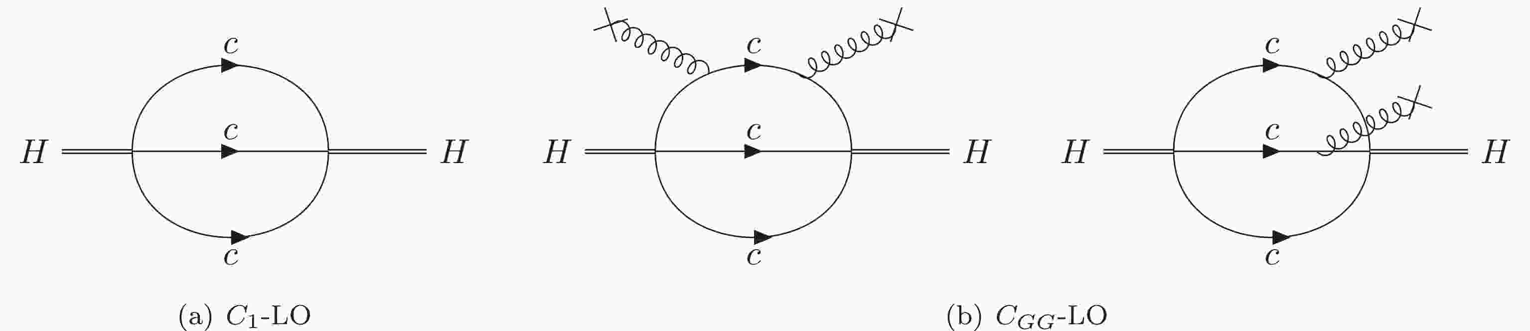
$ \alpha_s $ . For the OPE, we consider the most important contributions, i.e., perturbative term$ C_1 $ and the GG condensation,$ C_{GG} \langle g_s^2 \hat{G}\hat{G} \rangle $ , because other higher dimensional operators are power suppressed. According to Eq. (13), we need the imaginary parts of$ C_1 $ and$ C_{GG} $ , which can be calculated perturbatively.We use FeynArts [59, 60] to generate the Feynman diagrams and amplitudes of
$ C_1 $ and$ C_{GG} $ . The LO and NLO Feynman diagrams are shown in Fig. 1 and Fig. 2, respectively.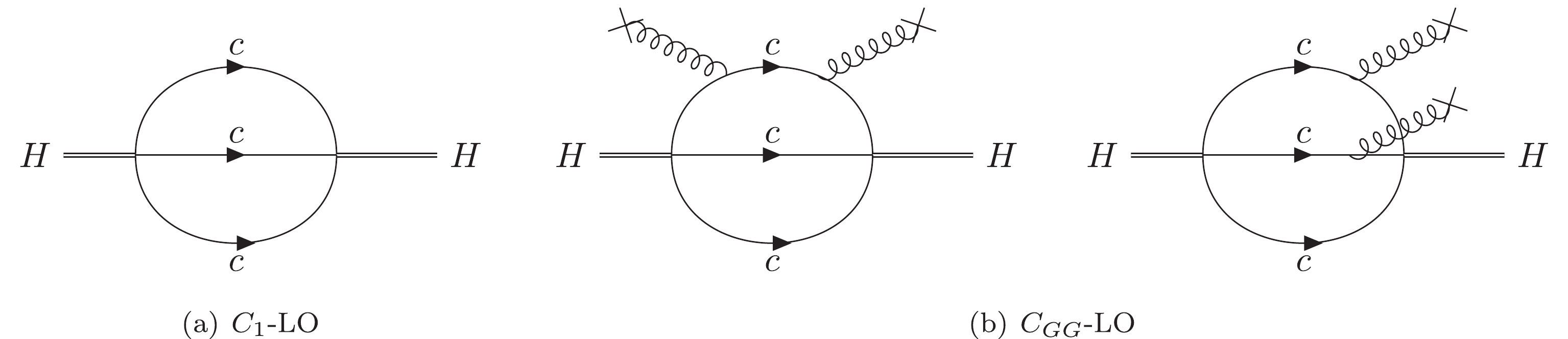
Figure 1. LO Feynman Diagrams of
$C_1$ and$C_{GG}$ . H denotes the interpolating current.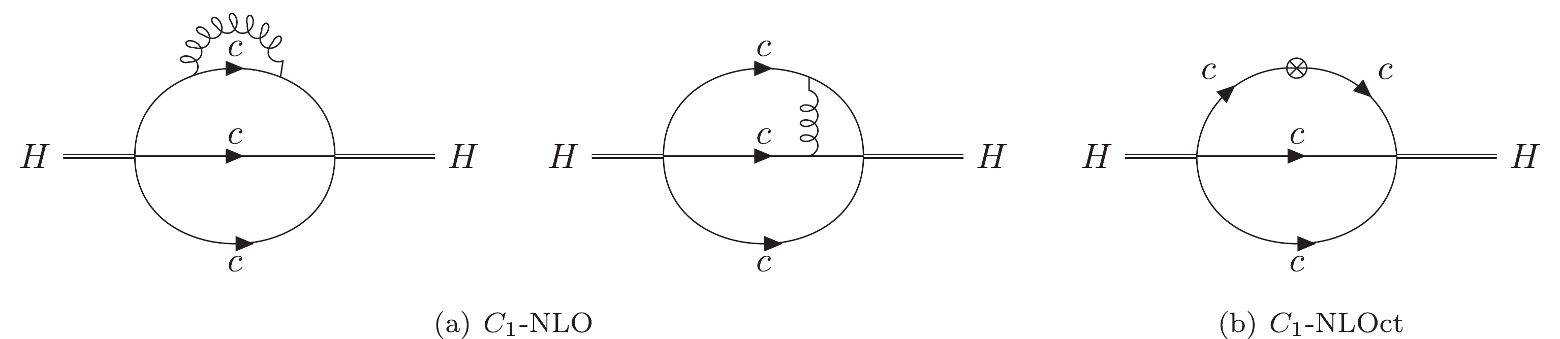
Figure 2. NLO and counter term Feynman Diagrams of
$C_1$ . H denotes the interpolating current.In the
$ \Omega_{QQQ} $ system, the three quarks have the same flavor, thus, some diagrams are similar and not shown again. For example, there are three cases in the second diagram of$ C_1 $ -NLO in Fig. 2, which denotes the cases with one gluon exchange between any two heavy quarks.The calculation procedures for
$ C_1 $ and$ C_{GG} $ are summarized below:1. We use FeynCalc [61, 62] to simplify the spinor structures of the Feynman amplitudes with the Naive-
$ \gamma_5 $ scheme.2. We use Reduze [63] to reduce all the loop integrals I to the linear combination
${\bf{I}} = \displaystyle\sum a_i\, \tilde{I}_i$ , where$ {\tilde{I}_i} '{\rm{s}}$ are the so-called master integrals (MIs). Furthermore,$ a_i $ s are the reduced coefficients, which are rational functions in the Mandelstam invariant (s), quark mass ($ m_Q $ ), and time-space dimension ($ D = 4-2\epsilon $ ) in this work.3. We set up differential equations for MIs [64-67] and solve them numerically, with boundary conditions obtained via the auxiliary mass flow method [68]. (The expressions of the MIs are the series-expansion forms, i.e.
$\tilde{I}(s,r,\epsilon) = s^{a+b\epsilon} \displaystyle\sum_{n,m} \left(\sum_{i} c_{mni} \epsilon^i\right){\rm Log}(r)^{m} r^{n}$ , where$ r = m_Q^2/s $ and$ c_{mni} {\rm{s}}$ are float numbers rather than rational numbers. The expressions of the Wilson coefficients$ C_1 $ and$ C_{GG} $ are complex and not presented in this paper. These results will be shared in auxiliary files.)4. Renormalization. There are no infrared divergences in the NLO amplitude of
$ C_1 $ . After performing the wave-function and mass renormalization of the quarks ($ m_Q $ is renormalized in either the$ \overline{\rm{MS}} $ or On-Shell scheme), the remaining ultraviolet divergences can be removed by the operator renormalization of current$ J_\mu $ . We renormalize the current in the$ \overline{\rm{MS}} $ scheme, and find the renormalizaion constant up to the NLO level as$ Z_{O} = 1+\frac{\alpha_s}{6 \pi }\left(\frac{1}{\epsilon}+\rm{Log}(4\pi)-\gamma_E \right)。 $

(14) -
In our numerical analysis, we choose the following parameters [54, 69-73].
$ \begin{aligned}[b] &m_c^{\overline{\rm{MS}}}(m_c) = 1.28 \pm 0.03\, \, {{\rm{GeV}}}\,\\ &m_c^{\rm OS} = 1.46 \pm 0.07\, \, {{\rm{GeV}}}\,\\ &m_b^{\overline{\rm{MS}}}(m_b) = 4.18 \pm 0.03\, \, {{\rm{GeV}}}\,\\ &m_b^{\rm OS} = 4.65 \pm 0.05\, \, {{\rm{GeV}}}\,\\ &\langle g_s^2 \hat{G}\hat{G} \rangle = 4\pi^2(0.037\pm0.015) \, \, {{\rm{GeV}}}^4 \,\\ &\alpha_s(m_Z = 91.1876 \; {{\rm{GeV}}}) = 0.1181 。 \end{aligned} $

(15) It is worth emphasizing that
$ \alpha_s (\mu) $ and the heavy quark mass,$ m_Q^{\overline{\rm{MS}}}(\mu) $ , are obtained through two-loop running [54]. As a typical and tentative choice, we set the renormalization scale, µ, to be equal to the Borel parameter,$ M_B $ in our phenomenological analysis [44, 74] (we will discuss the renormalization scale dependence of the results by setting µ with other values later). Moreover, the On-Shell (OS) masses$m_c^{\rm OS}$ and$m_b^{\rm OS}$ are extracted from the QCD sum rules analysis of the$ J/\psi $ and$ \Upsilon(1S) $ spectrums, respectively, in which the mass renormalization scheme and truncation order of$ \alpha_s $ are the same as ours.According to Eq. (13), the numerical result of
$ M_H $ depends on two parameters:$ s_0 $ and$ M_B $ . Principally,$ M_H $ as a physical mass, is independent of any artificial parameters. Therefore, a credible result should be obtained in an appropriate region of these two parameters, where$ M_H $ is dependent weakly on$ M_B $ and$ s_0 $ . Additionally, the choices of$ M_B $ and$ s_0 $ should ensure the validity of the OPE and dominance of the ground-state pole contribution, which will constrain the two parameters within a suitable parameter space, the so-called "Borel window". Within the Borel window, we find the so-called "Borel platform", in which$ M_H $ weakly depends on$ s_0 $ and$ M_B $ .To search for the Borel window, we define the relative contributions of the condensation and continuum as
$ \begin{aligned}[b]& r_{GG} = \frac{\langle g_s^2 \hat{G}\hat{G} \rangle\displaystyle\int_{s_{\rm{th}}}^{\infty} {\rm d}s \, \rho_{GG}(s)\, {\rm e}^{-\frac{s}{M_B^2}}}{\displaystyle\int_{s_{\rm{th}}}^{\infty} {\rm d}s \, \rho_{1}(s)\, {\rm e}^{-\frac{s}{M_B^2}}}\\ &r_{\rm{cont}} = \frac{\displaystyle\int_{s_0}^{\infty} {\rm d}s \, \rho_{1}(s)\, {\rm e}^{-\frac{s}{M_B^2}}}{\displaystyle\int_{s_{\rm{th}}}^{\infty} {\rm d}s \, \rho_{1}(s)\, {\rm e}^{-\frac{s}{M_B^2}}} \end{aligned} $

(16) and impose the following constraints:
$ |r_{GG}|\leqslant 30\%, \qquad |r_{\rm{cont}}|\leqslant 30\% \ . $

(17) The two constraints guarantee the validity of the OPE and the gound-state contribution dominance, separately. To find the Borel platform, we first search for the point on which the parameter dependence of
$ M_H $ is weakest within the Borel window. In addition to the conditions given in (17), we also impose the following constrain on$ s_0 $ :$ s_0<(M_H+1\; {\rm{GeV}})^2, $

(18) since
$ s_0 $ roughly denotes the energy scale where the continuum spectrum begins and the energy level spacing of a heavy hadron system is usually smaller than 1 GeV. More explicitly, we choose the variables as$ x = s_0 $ and$ y = M_B^2 $ and define the function describing the flatness degree as$ \Delta(x,y) = \left( \frac{\partial M_H}{\partial x}\right)^2+ \left ( \frac{\partial M_H}{\partial y}\right)^2\,. $

(19) Thus, minimizing the function
$ \Delta(x,y) $ within the Borel window and with the constrain (18), we obtain the point ($ x_0,y_0 $ ), which will be used to evaluate the central value of$ M_H $ . We then vary the values of$ s_0 $ and$ M_B^2 $ around the point ($ x_0,y_0 $ ) up to a 10% magnitude to estimate the errors of$ M_H $ . It should be emphasized that the central point ($ x_0,y_0 $ ) may lie on the margin of the Borel window in some cases, therefore, the parameter space used to estimate the errors of$ M_H $ may exceed the Borel window; additionally, the upper and lower errors are usually not symmetric. -
The results for
$ \Omega_{ccc}^{++} $ in the$ \overline{\rm{MS}} $ and OS schemes are listed in Table 1. The Borel platform curves, which show the parameter dependence of$ M_H $ on$ s_0 $ and$ M_B^2 $ , are shown in Fig. 3. In all the curves, the dot corresponds to the central point ($ x_0,y_0 $ ), and the shadows denote the Borel window determined by Eq. (17)Order $M_H$ /GeV

$s_0$ /

${\rm{GeV}}^2$ 

$M_B^2$ /

${\rm{GeV}}^2$ 

Error from $s_0$ and

$M_B^2$ 

Error from $m_Q$ 

Error from μ LO( $\overline{\rm{MS}}$ )

$4.39^{+0.24}_{-0.22}$ 

$29(\pm 10$ %)

$1.75(\pm 10$ %)

$^{+0.02}_{-0.03}$ 

$^{+0.10}_{-0.10}$ 

$^{+0.22}_{-0.19}$ 

NLO( $\overline{\rm{MS}}$ )

$4.53^{+0.26}_{-0.11}$ 

$26(\pm 10$ %)

$1.20(\pm 10$ %)

$^{+0.02}_{-0.04}$ 

$^{+0.09}_{-0.10}$ 

$^{+0.24}_{-0.00}$ 

LO(OS) $4.51^{+0.19}_{-0.23}$ 

$21(\pm 10$ %)

$0.40(\pm 10$ %)

$^{+0.06}_{-0.15}$ 

$^{+0.18}_{-0.18}$ 

NLO(OS) $4.55^{+0.13}_{-0.18}$ 

$22(\pm 10$ %)

$0.90(\pm 10$ %)

$^{+0.07}_{-0.12}$ 

$^{+0.11}_{-0.14}$ 

Table 1. LO and NLO results for the mass of
$\Omega_{ccc}^{++}$ in$\overline{\rm{MS}}$ and On-Shell schemes. Here, the errors for$M_H$ are from$s_0, M_B$ , the charm quark mass, and the renormalization scale μ with$\mu=kM_B$ and$k \in (0.8, 1.2)$ (the central values correspond to$\mu=M_B$ ).
Figure 3. (color online) Borel platform curves for the
$\Omega_{ccc}^{++}$ in$\overline{\rm{MS}}$ and On-Shell schemes.First, from Fig. 3, we observe that there exists a perfect Borel platform in the
$ \overline{\rm{MS}} $ scheme. However, there is no decent Borel platform in the OS scheme, thus, the result in the OS scheme is not good. Therefore, we consider the result in the$ \overline{\rm{MS}} $ scheme as our prediction for the mass of$ \Omega_{ccc}^{++} $ .Secondly, although the OS result is not good, we can still observe the distinct NLO effects in the reduction of the scheme dependence by the comparison between the
$ \overline{\rm{MS}} $ and OS schemes. In fact, at the LO a big gap is observed between the two schemes results, whereas the$ \overline{\rm{MS}} $ result increases markedly at the NLO, which brings the results of the two schemes close to each other at the NLO. Furthermore, the quark mass dependence of the results is also reduced at the NLO. Particularly, the NLO contribution leads to a noteworthy and significant correction of the LO result, and cannot be ignored in the QCD sum rules for the triply charmed baryons.Furthermore, as already mentioned, we will evaluate the renormalization scale µ dependence of the LO and NLO results in the
$ \overline{\rm{MS}} $ scheme. The results obtained with$ \mu = M_B $ are listed in Table 1. We then study the results with different µ ($ \mu = k \ M_B $ ) and$ k \in (0.8, 2.0) $ , which are presented in Fig. 4 and Table 2. The range of µ is chosen with the requirement that the Borel platform can be achieved and the perturbative expansion is under good control. From Fig. 4 it can be clearly observed that the µ dependence is significantly reduced for the NLO result, whereas the LO result is very sensitive to the choice of µ. Additionally, it is worth noting that the obtained NLO mass of$ \Omega_{ccc}^{++} $ is 4.75–4.80 GeV for a rather wide range of$ \mu = (1.2-2.0) M_B $ . Considering all important factors, like$ \mu $ dependence and perturbative convergence, 4.75-4.80 GeV is a more credible prediction for the$ \Omega_{ccc} $ mass. Interestingly enough, this value is in good agreement with the lattice QCD result.
Figure 4. (color online) Dependence on renormalization scale μ in
$\overline{\rm{MS}}$ scheme for$\Omega_{ccc}^{++}$ .k ( $\mu=k \ M_B$ )

$\rm LO$ /GeV

$\rm NLO$ /GeV

0.8 4.65 4.70 1.0 4.39 4.53 1.2 4.20 4.77 1.4 4.05 4.79 1.6 3.93 4.79 1.8 3.83 4.80 2.0 3.76 4.79 Table 2.
$\overline{\rm{MS}}$ mass of$\Omega_{ccc}$ with different renormalization scale$\mu=k M_B$ .It is worth mentioning that our result includes errors due to the variation of the renormalization scale, as compared with previous LO results [23, 25] (
$ 4.67 \pm0.15\; {{\rm{GeV}}} $ and$ 4.81 \pm 0.10\; {{\rm{GeV}}} $ , respectively, in which the scale dependence is not considered). Regarding the central values, the differences between our LO results and those in [23, 25] are mainly caused by the choice of input parameters and determination of the Borel platform. For example, we can reproduce the result in [25] using the parameters therein. In Table 5, we list the predictions for the mass of$ \Omega_{ccc}^{++} $ in various approaches. -
For the
$ \Omega_{bbb}^{-} $ , the results in the$ \overline{\rm{MS}} $ and OS schemes are listed in Table 3, and the Borel platform curves are shown in Fig. 5.Order $M_H$ /GeV

$s_0$ /

${\rm{GeV}}^2$ 

$M_B^2$ /

${\rm{GeV}}^2$ 

Error from $s_0$ and

$M_B^2$ 

Error from $m_Q$ 

Error from μ LO( $\overline{\rm{MS}}$ )

$13.97^{+0.54}_{-0.50}$ 

$224(\pm 10$ %)

$17.00(\pm 10$ %)

$^{+0.23}_{-0.36}$ 

$^{+0.06}_{-0.06}$ 

$^{+0.48}_{-0.34}$ 

NLO( $\overline{\rm{MS}}$ )

$14.27^{+0.33}_{-0.32}$ 

$232(\pm 10$ %)

$10.00(\pm 10$ %)

$^{+0.12}_{-0.25}$ 

$^{+0.08}_{-0.08}$ 

$^{+0.30}_{-0.19}$ 

LO(OS) $14.00^{+0.15}_{-0.15}$ 

$197(\pm 10$ %)

$0.40(\pm 10$ %)

$^{+0.01}_{-0.01}$ 

$^{+0.15}_{-0.15}$ 

NLO(OS) $14.06^{+0.10}_{-0.14}$ 

$200(\pm 10$ %)

$1.75(\pm 10$ %)

$^{+0.07}_{-0.07}$ 

$^{+0.07}_{-0.12}$ 

Table 3. LO and NLO results for the mass of
$\Omega_{bbb}^{-}$ in$\overline{\rm{MS}}$ and On-Shell schemes. Here, the errors for$M_H$ are from$s_0, M_B$ , the bottom quark mass, and renormalization scale μ with$\mu=kM_B$ and$k \in (0.8, 1.2)$ (the central values correspond to$\mu=M_B$ ).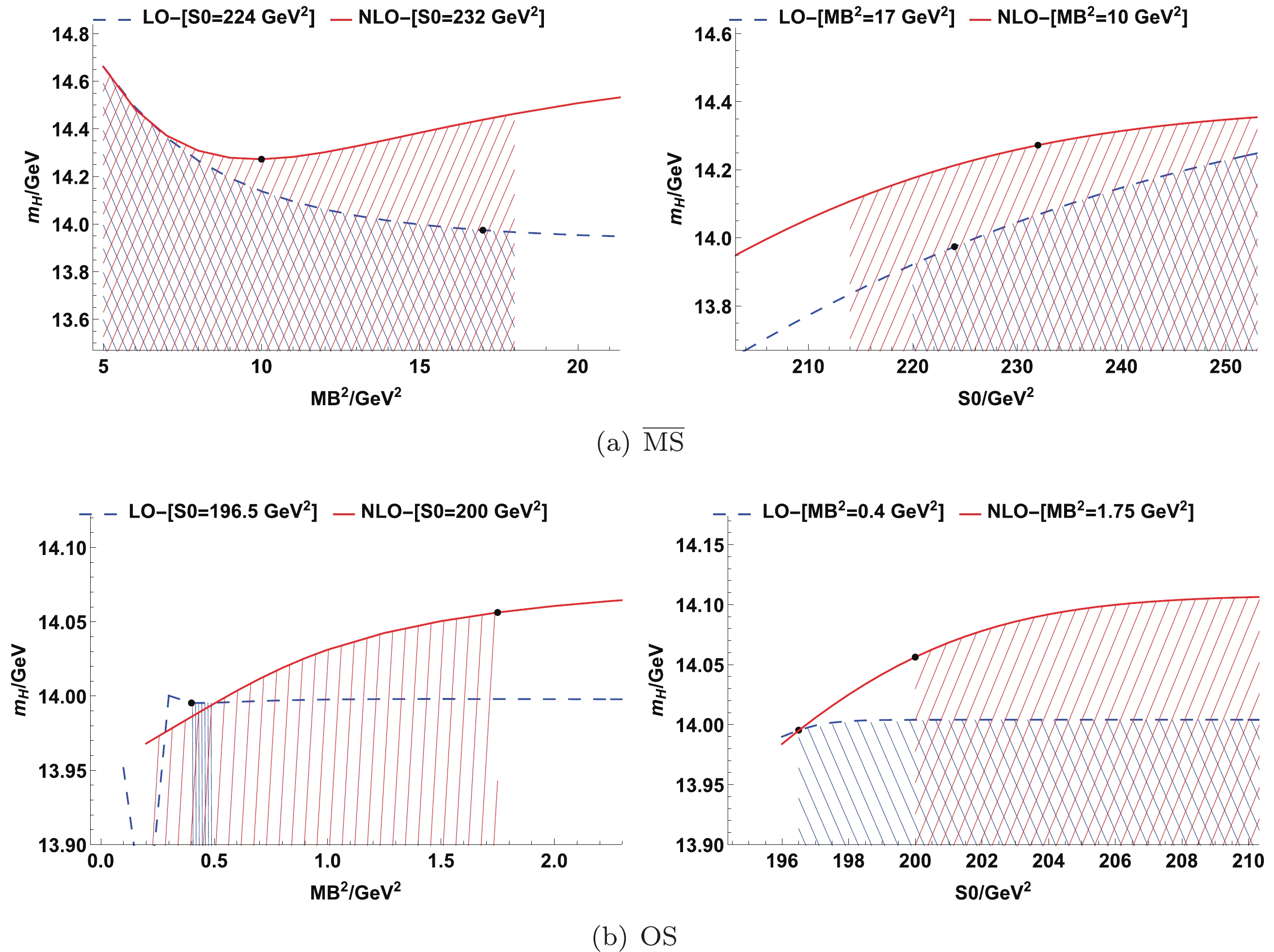
Figure 5. (color online) Borel platform curves for the
$\Omega_{bbb}^{-}$ in$\overline{\rm{MS}}$ and On-Shell schemes.With these figures, we can make similar conclusions as illustrated in the ccc section. For instance, there are no very stable Borel platforms in the OS scheme at both the LO and NLO. Furthermore, there is a distinct difference between the bbb and ccc systems. This can be observed in Fig. 5, where there is no Borel platform at the LO in the
$ \overline{\rm{MS}} $ scheme; however, there appears a clear platform after including the NLO contribution. For the ccc, there are platforms at both the LO and NLO. This indicates that for the bbb the NLO contribution from the perturbative term$ C_1 $ is crucial to the formation of a stable Borel platform in the QCD Sum Rules.k ( $\mu=k \ M_B$ )

$\rm LO$ /GeV

$\rm NLO$ /GeV

0.8 14.45 14.57 1.0 13.97 14.27 1.2 13.63 14.08 1.4 13.34 13.96 Table 4.
$\overline{\rm{MS}}$ mass of$\Omega_{bbb}$ with different renormalization scale$\mu=k M_B$ .We further evaluate the renormalization scale µ dependence of the
$ \Omega_{bbb}^{-} $ mass in a wider range of$ \mu = (0.8-1.4)M_B $ ($ \mu>1.4 M_B $ is excluded owing to the absence of the Borel platform), and the results are shown in Fig. 6 and Table 4. It can be observed that the scale dependence is obviously weaker at the NLO than at the LO. Nevertheless, at the NLO, the uncertainty for the$ \Omega_{bbb}^{-} $ mass due to the scale dependence is still not small. This implies that all estimates of the masses at the LO in the QCD sum rules must suffer from large uncertainties caused by the scale dependence, and can be improved by including the NLO contributions.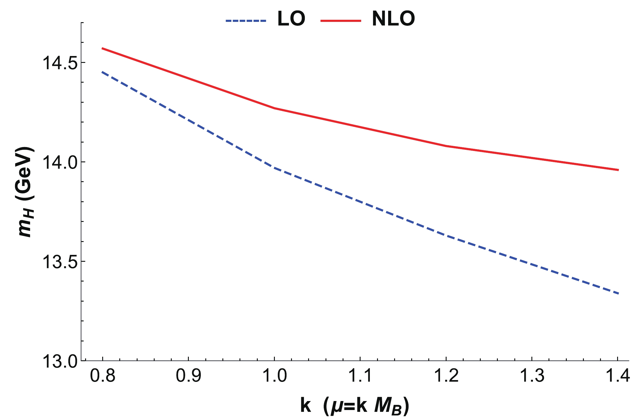
Figure 6. (color online) Dependence on renormalization scale μ in
$\overline{\rm{MS}}$ scheme for$\Omega_{bbb}^{-}$ .Our result for the
$ \Omega_{bbb}^{-} $ mass at the LO ($ 13.97^{+0.54}_{-0.50} $ GeV) is comparable with previous works in QCD sum rules at the LO [23, 25] ($ 13.28 \pm0.10\; {{\rm{GeV}}} $ and$ 14.43 \pm0.09\; {{\rm{GeV}}} $ respectively), which is similar to the case of$ \Omega_{ccc}^{++} $ . Theoretical uncertainties are significantly reduced after considering the NLO contribution. We then obtain$ 14.27^{+0.33}_{-0.32} $ GeV at the NLO in the$ \overline{\rm{MS}} $ scheme. The results obtained in various approaches are listed in Table 5, all of which are comparable with our results. -
In this work, we also evaluate the GGG condensate contributions, and find that they are very small; thus, they do not affect the phenomenological results.
The leading order contributions of the GGG condensate come from two parts: one is from the diagrams shown in Fig. 7 and the other is from the higher order of the gluons background field in the
$ C_{GG} $ -LO of Fig. 1, i.e.,$ \langle GGG\rangle $ that is related to the$ \langle A(x)A(y)\rangle $ expansion. (Similar to the results of$ C_1 $ and$ C_{GG} $ , the results of$ C_{GGG} $ will be shared by auxiliary files). Choosing$ \langle g_s^3 \hat{G}\hat{G}\hat{G} \rangle\ = $ $ \ 0.054 \pm 0.014 {\rm{GeV}}^6 $ [25, 45-47], similar to [25], we find the ratios of different condensate contributions near the Borel platform as
Figure 7. Part contribution of
$C_{GGG}$ -LO. H denotes the interpolating current.$ \begin{aligned}[b]&\int_{s_{\rm{th}}}^{s_0} {\rm d}s \ \rho_{1}(s)\ {\rm e}^{-\frac{s}{M_B^2}} : \ \int_{s_{\rm{th}}}^\infty {\rm d}s \ \rho_{GG}(s) \langle g_s^2 \hat{G}\hat{G} \rangle \ {\rm e}^{-\frac{s}{M_B^2}}\ : \\ &\ \ \int_{s_{\rm{th}}}^\infty {\rm d}s \ \rho_{GGG}(s) \langle g_s^3 \hat{G}\hat{G}\hat{G} \rangle \ {\rm e}^{-\frac{s}{M_B^2}}\ \simeq \ 1\, : {\cal{O}}(10^{-2}) : {\cal{O}}(10^{-4}) \end{aligned}$

(20) Even if we use a larger value of
$ \langle g_s^3 \hat{G}\hat{G}\hat{G} \rangle\ = \ 0.52 \pm $ $ 0.10 \;{\rm{GeV}}^6 $ as chosen in [75-78], we can still observe that this d = 6 GGG condensate contributions are still too small to affect the phenomenological results. This conclusion is consistent with the findings in Ref. [25]. Therefore, according to our study, the GGG condensate contributions can be ignored. -
In the study of hadron physics, the QCD sum rule is known to be a powerful tool to evaluate hadron properties. For the triply heavy baryons
$ QQQ \; (Q = c,b) $ , previous works only dealt with the LO perturbative QCD calculation. The absence of the higher order QCD corrections may lead to large theoretical uncertainties in the QCD sum rules. In this paper, for the first time, we calculate the NLO QCD contribution of the QQQ system by considering the NLO correction to the perturbative term of$ C_1 $ in the OPE. Additionally, the non perturbative contribution is embodied by the d = 4 gluon-gluon condensate. We also introduce adequate constraints to ensure the ground state dominance and power suppressions within the Borel windows.Because the main theoretical uncertainty of the LO result is from the absence of the NLO correction of
$ C_1 $ in the QCD sum rules, the inclusion of the NLO contribution plays important roles theoretically and phenomenologically. By comparing the NLO result with the LO one, we may draw the following conclusions for the$ \Omega_{QQQ} $ system. First, the correction from the NLO contribution is sizable ($\Delta M_H = $ $ M_H^{\rm NLO}\, -\, M_H^{\rm LO}$ can be as large as$0.2 \sim $ $ 0.3\;{\rm GeV}$ or even larger). Secondly, after considering the NLO contribution, the parameters dependence of the results is reduced and the Borel platform becomes more distinct, especially for the bbb system in the$ \overline{\rm{MS}} $ scheme. Thirdly, the dependences on the renormalization schemes and quark masses are significantly improved for the$ \Omega_{ccc} $ .By including the NLO contribution of the perturbative part in the QCD sum rules, we find the masses to be
$ 4.53^{+0.26}_{-0.11} $ GeV for$ \Omega_{ccc} $ and$ 14.27^{+0.33}_{-0.32} $ GeV for$ \Omega_{bbb} $ , where the results are obtained at$ \mu = M_B $ with errors including that from the variation of the renormalization scale µ in the range$ (0.8-1.2) M_B $ . Further study for the µ dependence in a wider range shows that the LO results are very sensitive to the choice of µ, and therefore have large uncertainties, whereas the NLO results are considerably better. Aside from the masses given above at$ \mu = M_B $ (in Table 5), a quite stable value, (4.75–4.80) GeV, for the$ \Omega_{ccc} $ mass is found in the range of$ \mu = (1.2-2.0) M_B $ . The distinctions between the LO and NLO results on the renormalization scale can be most clearly observed in Table 2 and Fig. 4 for the$ \Omega_{ccc} $ . Considering all important factors, like$ \mu $ dependence and perturbative convergence, 4.75-4.80 GeV is a more credible prediction for the$ \Omega_{ccc} $ mass. Finally, we also evaluate the d = 6 GGG condensate contributions, which are found to be so small that they can be ignored in the phenomenological analysis.Therefore, in our view, the NLO contribution is indeed important and should not be ignored. Further evaluations on the NLO corrections, e.g., to the coefficient
$ C_{GG} $ of the two gluon condensation, may be needed, which will be helpful to constrain the theoretical errors for the nonperturbative contributions. -
We thank Chen-Yu Wang, Xiao Liu, and Xin Guan for the many useful and helpful discussions. We also thank Shi-Lin Zhu for the helpful comments.
-
The definition of the baryon operator is shown as follows,
$ {\cal{O}}_{\Gamma_1,\Gamma_2} = \epsilon_{ijk}\left( (q_1^i)^T \hat{C}\Gamma_1 q_2^j \right)\Gamma_2 q_3^k \tag{A1}$

and the next-to-leading order correction excluding the quark self-energy diagram, can be divided into two parts,
$ A = \int \frac{d_p^D}{(2\pi)^D}(A_1+A_2)\ , \tag{A2}$

where
$ A_1 $ denotes the case of the exchanging gluon between quarks$ q_1 $ and$ q_2 $ , and$ A_2 $ denotes the other cases of the exchanging gluon between quarks$ q_1 $ and$ q_3 $ and$ q_2 $ and$ q_3 $ . The corresponding amplitudes are$\begin{aligned}[b] A_{1} =& \!\epsilon_{ijk} \left[\!{\rm i} g_s \gamma_{\mu} \frac{-{\rm i}\not\!\!{p}}{p^{2}}\!\Gamma_{1} \frac{{\rm i}\not\!\!{p}}{p^{2}} {\rm i} g_s \gamma^{\mu} \left(T^{a}\right)_{i i^{\prime}}\left(T^{a}\right)_{j j^{\prime}}\!\right]\\&\times \left[\Gamma_{2} \delta_{k k^{\prime}} \!\right] \frac{-{\rm i}}{p^{2}}\ ,\end{aligned} \tag{A3}$

$\begin{aligned}[b] A_{2} = &\epsilon_{ijk}\left[{\rm i} g_s \gamma_{\mu} \frac{-{\rm i}\not\!\!{p}}{p^{2}} \Gamma_{1} \left(T^{a}\right)_{i i^{\prime}} \delta_{j j^{\prime}} \right.\\ &\left.+\Gamma_{1} \frac{-{\rm i}\not\!\!{p}}{p^{2}} {\rm i} g_s \gamma_{\mu} \delta_{i i^{\prime}}\left(T^{a}\right)_{j j^{\prime}} \right]\\&\times \left[\Gamma_{2} {\rm i} g_s \gamma^{\mu} \frac{{\rm i}\not\!\!{p}}{p^{2}} \left(T^{a}\right)_{k k^{\prime}} \right] \frac{-{\rm i}}{p^{2}}\ ,\end{aligned} \tag{A4}$

Because there are no residual infrared (IR) divergences, we only need to consider ultraviolet (UV) divergences. Therefore, the mass terms are ignored in quark propagators.
Then we can get the following form after the reduction:
$ A = -{\rm i} g_s^2 \frac{1}{D} \int \frac{d_p^D}{(2\pi)^D}\ \frac{1}{(p^2)^2}\ B\ , \tag{A5}$

where
$ \begin{aligned}[b] B =& -\left(\gamma_{\mu} \gamma_{\nu} \Gamma_{1} \gamma^{\nu} \gamma^{\mu}\right)\left(\Gamma_{2}\right)\left(T^{a}\right)_{i i^{\prime}}\left(T^{a}\right)_{j j^{\prime}} \delta_{k k^{\prime}}\epsilon_{ijk} \\ &-D \left(\Gamma_{1}\right)\left(\Gamma_{2}\right)\left[\left(T^{a}\right)_{i i^{\prime}} \delta_{j j^{\prime}}+\delta_{i i^{\prime}}\left(T^{a}\right)_{j j^{\prime}}\right]\left(T^{a}\right)_{k k} \epsilon_{ijk}\\ &-\!\frac{1}{2}\left(\left[\sigma_{\mu \nu}, \Gamma_{1}\right]\right)\left(\!\Gamma_{2} \sigma_{\mu \nu}\!\right)\left[\!\left(T^{a}\right)_{i i^{\prime}} \delta_{j j^{\prime}}\!+\!\delta_{i i^{\prime}}\left(T^{a}\right)_{j j^{\prime}}\!\right]\left(T^{a}\right)_{k k^{\prime}}\epsilon_{ijk}\ . \end{aligned} \tag{A6}$

According to Eq. (A5), we can get the UV divergences part of A.
$ A_{UV} = -\left.{\rm i} g_s^{2} \frac{1}{4} \frac{{\rm i}}{(4 \pi)^{2}} \frac{1}{\varepsilon} B\right|_{D = 4} = \frac{\alpha_{s}}{\varepsilon} \frac{\left.B\right|_{D = 4}}{16\pi}\ , \tag{A7}$

$ A_{UV} $ is canceled by the operator renormalization term and renormalization coefficients of the quark wave function from operator$ {\cal{O}}_{\Gamma_1,\Gamma_2} $ , thus, the corresponding operator renormalization term in$ \overline{\rm{MS}} $ scheme is$ Z_O = 1+\delta Z_O = 1+ \delta \left( \frac{1}{\epsilon}+{\rm Log}(4\pi)-\gamma_E \right) \ , \tag{A8}$

where
$ \delta = - \alpha_s \frac{\left.B\right|_{D = 4}}{16\pi}- 3\left(-\frac{1}{2} \frac{\alpha_s}{3\pi} \right) {\bf{I}}\ .\tag{A9} $

where I denotes the identity matrix.
At last, in this work, we can use the following relation, gotten by the Fierz transformation.
$ \epsilon_{ijk}\left( (Q^i)^T \hat{C}\gamma_\lambda Q^j \right) \sigma_{\lambda \mu} Q^k\ = \ {\rm i}\ \epsilon_{ijk}\left( (Q^i)^T \hat{C}\gamma_\mu Q^j \right) Q^k.\tag{A10} $

This relation is valid in the D dimension, (
$ D = 4-2\epsilon $ ).
NLO effects for ΩQQQ baryons in QCD Sum Rules
- Received Date: 2021-06-09
- Available Online: 2021-09-15
Abstract: We study the triply heavy baryons


 DownLoad: