


 Abstract
 HTML
HTML Reference
 Related
 PDF
PDF


-
In classical general relativity, the problem of singularities has remained unresolved since it was pointed out by Penrose and Hawking [1, 2]. The reason why physicists hate singularities is primarily because their existence will lead to incomplete geodesics, so that the causality is destroyed. However, the strong belief in the inevitability of causality indicates that classical general relativity fails and quantum effects must be considered around the singularity. Along this line, some interesting studies have been reported in recent years [3-7].
Quantum corrected black holes seem to be different from classical black holes in terms of the photon sphere and shadows because the quantum effect is significant in the strong gravitational regime. For spherically symmetric black holes in classical general relativity, much evidence shows that the radii of the horizon
$ r_0 $ , shadow$ b_c $ , and outermost photon sphere$ r_{ph} $ obey a universal conjecture [8, 9]$ \frac{3}{2}r_0\leqslant r_{ph}\leqslant\frac{b_c}{\sqrt{3}}\leqslant 3M , $

(1) where M is the mass of the black hole. Later, these inequalities were proved for asymptotically flat black holes, which satisfy the null energy condition in the framework of Einstein gravity in [10]. However, by considering the spherically symmetric black hole in regularized
$ 4D $ Einstein-Gauss-Bonnet (EGB) gravity, the authors found that the relations are reversed when the GB coupling constant is negative [11, 12], viz.,$ \frac{3}{2}r_0\geqslant r_{ph}\geqslant\frac{b_c}{\sqrt{3}}\geqslant 3M . $

(2) In addition, a regularized
$ 4D $ EGB black hole can also be obtained by considering the conformal anomaly of Einstein gravity [13]. Moreover, the violation of inequalities (1) was found in [14] for Einsteinian cubic gravity and in [15] for Einsteinian quartic gravity. It is worth noting that these theories, such as the string theory, are all well posed higher derivative gravities that would naturally arise for ultraviolet complete quantum gravity. Hence, one may guess that the quantum effect may cause inequality (1) to flip. In general, an exact black hole solution is difficult to obtain when considering quantum modification. In the first part of this paper, we consider a simple quantum corrected Schwarzschild black hole obtained by Kazakov and Solodukhin [16] to test this conjecture. In fact, the shadow radius of a Kazakov-Solodukhin (KS) black hole has already been obtained in [17], but the above inequality sequence has not been examined.A shadow is a dark area that is formed when an opaque body prevents the transmittance of light. By definition, the shape of a shadow depends on the location and intensity of the light source. The same is true for black hole shadows. For the standard usage of the term "shadow", the light source is thought to be distributed throughout the space randomly, including from behind the observer. However, if a particular light source (like an accretion disk) near the black hole is so bright that the natural light sources can be ignored, the appearance of a black hole cannot be described by the standard "shadow". Recently, Gralla et al. presented an elegant description of the observational appearance of a black hole when considering the emission disk around it [18]. To avoid ambiguity, the standard "shadow" is suggested to be called the "critical curve" [18]. For example, the shadow we mentioned in the inequalities in the previous paragraph is the critical curve. In this context, the observed size of the central dark area is primarily governed by the emission profile and gravitational redshift; however, the general physical information is encoded in the so called photon and lensing rings [18-22]. In addition, the optical appearance of a star orbiting a black hole is also an interesting topic to study, see examples in [23-32]. Furthermore, the shadow of a black hole observed by other physical observers also has people's attention, some interesting results can be found in [33-36].
Our main motivation is to provide observational evidence for the reversed inequality (2) based on the work of Gralla et al. In Section II, we obtain the radius of a photon sphere and shadow of a KS black hole and verify the inverse inequalities (2). In Section III, we analyze the light bending in a KS black hole. In Section IV, we calculate the innermost stable circular orbit (ISCO) in a KS black hole. In Section V, we consider thin disk emission near the black hole and investigate the observational appearance with three typical emission profiles. We conclude in Section VI.
-
Kazakov and Solodukhin showed that when considering spherically symmetric quantum fluctuations of a Schwarzschild black hole, the
$ 4D $ theory of gravity with Einstein action reduces to the effective$ 2D $ dilaton gravity [16]$ S = -\frac{1}{8}\int {\rm d}^2z\sqrt{-g}\left[r^2R^{(2)}-2(\nabla r)^2+\frac{2}{G_N}U(r)\right] . $

(3) Here,
$ R^{(2)} $ is the two-dimensional Ricci scalar,$ G_N $ is the Newtonian constant, and$ U(r) $ is the dilaton potential. A solution for this action is a Schwarzschild-like metric$ {\rm d}s^2 = -f(r){\rm d}t^2+\frac{{\rm d}r^2}{f(r)}+r^2{\rm d}\Omega^2_2,~ f(r) = -\frac{2M}{r}+\frac{1}{r}\int^rU(\rho){\rm d}\rho , $

(4) The non-trivial issue is to find a potential
$ U(r) $ such that the$ 2D $ dilaton theory is renormalizable. Kazakov and Solodukhin found that a renormalizable potential takes the form [16]$ U(r) = \frac{r}{\sqrt{r^2-16G_R}}, $

(5) where
$ G_R $ is the renormalized Newton constant. Defining a new parameter$ a = 4\sqrt{G_R} $ , we obtain the metric function for a quantum corrected Schwarzschild black hole$ f(r) = -\frac{2M}{r}+\frac{\sqrt{r^2-a^2}}{r} . $

(6) For an empty space with no quantum fluctuations,
$ U(r) = 1 $ and the metric is reduced to the Schwarzschild one. The central point-like singularity of the Schwarzschild black hole, which was originally at$ r = 0 $ , is now shifted to a central 2-dimensional spherical region with radius a that is of the order of the Planck length. In this sense, the quantum corrected Schwarzschild black hole renders the spacetime regular. The horizon is located at$ r_0 = \sqrt{4M^2+a^2} . $

(7) Although the metric is finite at
$ r = a $ , the curvature is divergent on this two-dimensional sphere. This is because the reducing procedure is not a complete quantum scheme for$ 4D $ gravity.The orbit of one particle traveling in curved spacetime is described by geodesic equations, which can be expressed as the Euler-Lagrange equation
$ \frac{{\rm d}}{{\rm d}\tau}\left(\frac{\partial{\cal L}}{\partial \dot x^\mu}\right) = \frac{\partial{\cal L}}{\partial x^\mu}, $

(8) where
$ \tau $ is the proper time,$ \dot x^\mu $ is the four-velocity of the particle, and$ {\cal L} $ is the Lagrangian. For the line element (4), the Lagrangian is$ {\cal L} = \frac{1}{2}g_{\mu\nu}\dot x^\mu\dot x^\nu = \frac{1}{2}\left(-f\dot t^2+\frac{\dot r^2}{f}+r^2\dot\theta^2+r^2\sin^2\theta\dot\phi^2\right). $

(9) For a static and spherically symmetric metric, we can always restrict the particle to move on the equatorial plane, i.e.,
$ \theta = \dfrac{\pi}{2} $ and$ \dot\theta = 0 $ . In addition, the Lagrangian$ {\cal L} $ does not involve coordinates t and$ \phi $ explicitly, so we have two conserved quantities$ E = -\frac{\partial{\cal L}}{\partial\dot t} = f\dot t,\quad L = \frac{\partial{\cal L}}{\partial\dot\phi} = r^2\dot\phi, $

(10) as the respective energy and angular momentum of one particle travelling around the black hole. For the null geodesic
$ {\cal L} = 0 $ , we can then obtain the orbit equation$ \left(\frac{{\rm d}r}{{\rm d}\phi}\right)^2+V_{\rm eff} = 0 , $

(11) with the effective potential given by
$ V_{\rm eff} = -r^4\left(\frac{1}{b^2}-\frac{f(r)}{r^2}\right), $

(12) where
$ b = \dfrac {L}{E} $ is called the impact parameter. The circular orbit corresponds to$ V_{\rm eff} = 0,\quad V'_{\rm eff} = 0. $

(13) Because of the spherical symmetry, all circular orbits form a closed surface, which is the so called photon sphere, whose radius is determined by
$ \left(\frac{f(r_{ph})}{r_{ph}^2}\right)' = 0 $

(14) and the corresponding impact parameter,
$ b_c $ , gives the standard shadow radius$ b_c = \frac{r_{ph}}{\sqrt{f(r_{ph})}} . $

(15) For a KS black hole (6), the photon sphere and shadow radius are respectively
$ r_{ph} = \sqrt{\frac{3(3+x^2+\sqrt{9+2x^2})}{2}}M, $

(16) $ b_c = \sqrt{\frac{\sqrt{27(3+x^2+\sqrt{9+2x^2})^3}}{2\sqrt{9+x^2+3\sqrt{9+2x^2}}-4\sqrt2}}M ,$

(17) where we introduce a dimensionless parameter
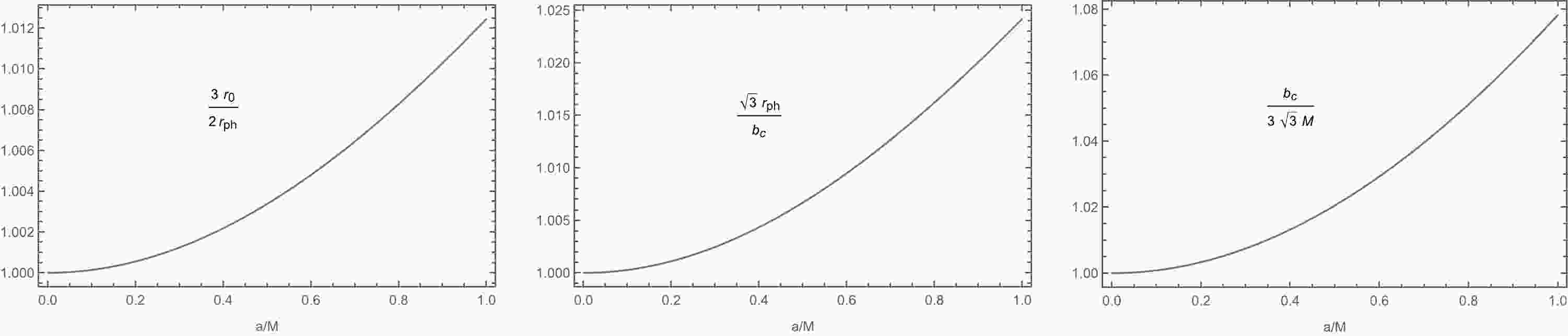
$ x = a/M $ . The shadow radius of a KS black hole has already been obtained in [17]. It is easy to show that for a KS black hole, we have the reversed inequalities$ \frac32r_0 \geqslant r_{ph} \geqslant \frac{b_c}{\sqrt3} \geqslant 3M , $

(18) as we have guessed in the introduction. We also show these inequalities in Fig. 1 explicitly. These facts support the idea that conjecture (1) proposed in [8, 9] will be destroyed when considering the quantum effect. An underlying reason may be that the quantum effect usually invalidates the null energy condition. As mentioned in the introduction, the violation of conjecture (1) is also common in higher derivative gravities. We do not have a well posed energy condition in higher derivative gravities because the energy momentum tensor is not simply connected with the Einstein tensor. In other words, the energy conditions have no definite physical significance in higher derivative gravities. At any rate, the quantum effects of both matter and gravity may destroy conjecture (1).
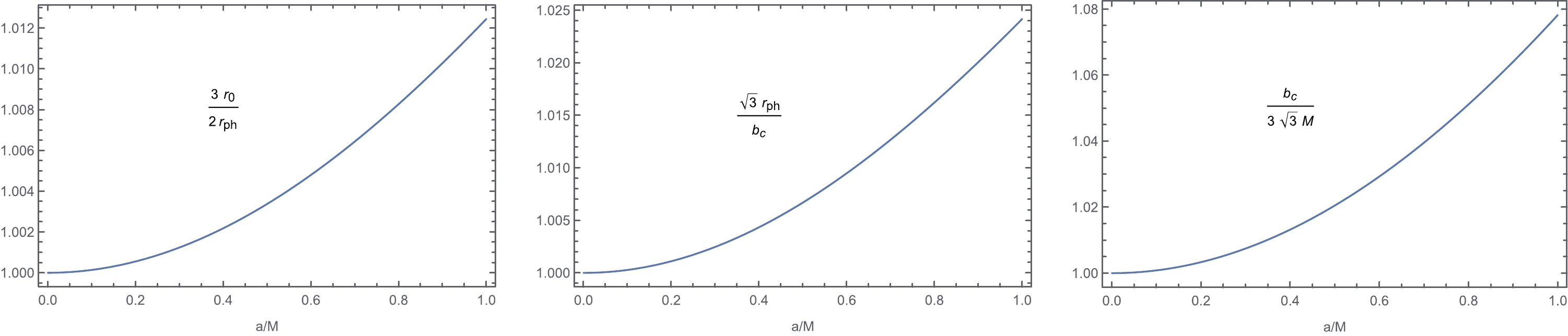
Figure 1. (color online) Plots of the ratios between
$ r_0, r_{ph} $ , and$ b_c $ with respect to the deformation parameter a for a KS black hole. -
In this section, to have a fuller understanding of the appearance of a KS black hole, we proceed to study the black hole shadow, photon rings, and lensing rings of a KS black hole around an accretion disk that has very high brightness. We begin by investigating the trajectory of a light ray traveling around the black hole. It is convenient to make the transformation
$ u = 1/r $ . The orbit equation now becomes$ \left(\frac{{\rm d}u}{{\rm d}\phi}\right)^2 = G(u), $

(19) where
$ G(u) = \frac{1}{b^2}+2Mu^3-u^2\sqrt{1-a^2u^2}. $

(20) When impact parameter
$ b>b_c $ , the light ray move towards the black hole from infinity, approaching one closest point, and then moves away from the black hole back to infinity. When impact parameter$ b<b_c $ , the light ray always falls into the black hole. When$ b = b_c $ , the light ray will revolve around the black hole at radius$ r_c $ , i.e., the photon sphere.For
$ b>b_c $ , the turning point corresponds to the minimally positive real root of$ G(u) = 0 $ , which we denote as$ u_m $ . According to (19), the total change in azimuthal angle$ \phi $ for a certain trajectory with impact parameter b can be calculated by$ \phi = 2\int_0^{u_m}\frac{{\rm d}u}{\sqrt{G(u)}},\quad b>b_c . $

(21) For
$ b<b_c $ , we only focus on the trajectory outside the horizon, so the total change in azimuthal angle$ \phi $ is obtained by$ \phi = \int_0^{u_0}\frac{{\rm d}u}{\sqrt{G(u)}},\quad b<b_c, $

(22) where
$ u_0 = 1/r_0 $ .To discuss the observational appearance of emission originating near a black hole, the authors in [18] divided trajectories into direct, lensed, and photon rings. Herein, we give a brief introduction. The total number of orbits can be defined as
$ n = \dfrac{\phi}{2\pi} $ , which is obviously a function of impact parameter b. We denote the solution of$ n(b) = \frac{2m-1}{4},\quad m = 1,2,3,\cdots$

(23) by
$ b_m^\pm $ . Note that$ b_m^-<b_c $ and$ b_m^+>b_c $ . Then, we can classify all trajectories as follows:● direct:
$ \dfrac{1}{4}<n<\dfrac{3}{4} \Rightarrow b\in(b_1^-,b_2^-)\cup(b_2^+,\infty) $ ● lensed:
$ \dfrac{3}{4}<n<\dfrac{5}{4} \Rightarrow b\in(b_2^-,b_3^-)\cup(b_3^+,b_2^+) $ ● photon ring:
$ n>\dfrac{5}{4} \Rightarrow b\in(b_3^-,b_3^+) $ The physical picture of this classification is clear from the trajectory plots in Fig. 2. Assuming light rays are emitted from the north pole direction (far right of the trajectory plots), trajectories whose number of orbits
$ 1/4<n<3/4 $ will intersect the equatorial plane only once. Trajectories with$ 3/4<n<5/4 $ number of orbits will intersect the equatorial plane twice. Trajectories with$ n>5/4 $ number of orbits will intersect the equatorial plane at least 3 times.
Figure 2. (color online) Behavior of photons in a KS black hole as a function of impact parameter b. On the left, we plot the total number of orbits
$ n = \phi/2\pi $ . The colors correspond to$ n<3/4 $ (black),$ 3/4<n<5/4 $ (yellow), and$ n>5/4 $ (red), defined as the direct, lensed, and photon ring trajectories, respectively. On the right, we show a selection of associated photon trajectories in the Euclidean polar coordinates$ (r,\phi) $ . The impact parameter spacing is 1/10, 1/100, and 1/1000 in the direct (black), lensed (yellow), and photon ring (red) bands, respectively. The black hole is shown as a solid disk. We have set$ M = 1, a = 0.5 $ . -
For the time-like geodesic
$ {\cal L} = -1/2 $ , the orbit equation is$ \left(\frac{{\rm d}r}{{\rm d}\phi}\right)^2+V_{\rm eff} = 0, $

(24) with the effective potential given by
$ V_{\rm eff} = -r^4\left(\frac{E^2}{L^2}-\frac{f(r)}{L^2}-\frac{f(r)}{r^2}\right). $

(25) The innermost stable circular orbit (ISCO) is determined by
$ V_{\rm eff} = 0,\quad V'_{\rm eff} = 0,\quad V''_{\rm eff} = 0 . $

(26) The solution
$r_{\rm isco}$ is one root of a quartic equation. Its expression is complicated, but we can numerically show that$r_{\rm isco} > 6M$ . Some other characteristics of the particle motion around a KS black hole, such as the frequencies at the ISCO, were considered in [37]. Here we list various important physical quantities for different deformation parameter a in Table 1.a $r_0$ 

$r_{ph}$ 

$r_{\rm isco}$ 

$b_c$ 

$b_1^-$ 

$b_2^-$ 

$b_2^+$ 

$b_3^-$ 

$b_3^+$ 

0 2 3 6 5.19615 2.8477 5.01514 6.16757 5.18781 5.22794 0.1 2.0025 3.00333 6.0075 5.20048 2.85105 5.01969 6.1713 5.19216 5.2322 0.5 2.06155 3.08193 6.18467 5.30259 2.93025 5.12696 6.25978 5.29484 5.33276 1 2.23607 3.31284 6.7086 5.60259 3.16347 5.44062 6.5239 5.59624 5.62886 Table 1. Various involved physical quantities for different values of deformation parameter a with
$M=1$ . -
Usually, the term "shadow" describes the appearance of a black hole illuminated from all directions; therefore, the shadow radius is given by critical impact parameter
$ b_c $ . In practice, the emission is always accumulated in a certain finite region near the black hole, such as an accretion disk. Armed with the previous preparations, now we are ready to consider a concrete accretion disk around a KS black hole on the equatorial plane. There are many models in accretion disk theory; however, we focus on optically and geometrically thin disks for simplicity.A static observer is assumed to be located at the north pole, and the light emitted from the accretion disk is considered isotropic in the rest frame of the static observer. In view of the spherical symmetry of spacetime, we also suppose the emitted specific intensity only depends on the radial coordinate, denoted by
$ I^{\rm em}_\nu(r) $ , with emission frequency$ \nu $ in a static frame. An observer at infinity will receive the specific intensity$ I^{\rm obs}_{\nu'} $ with redshifted frequency$ \nu' = \sqrt{f}\nu $ . Considering$ I_\nu/\nu^3 $ is conserved along a ray, i.e.,$ \frac{I^{\rm obs}_{\nu'}}{\nu'^3} = \frac{I^{\rm em}_\nu}{\nu^3} , $

(27) we have the observed specific intensity
$ I^{\rm obs}_{\nu'} = f^{3/2}(r)I^{\rm em}_\nu(r) . $

(28) Therefore, the total observed intensity is an integral over all frequencies
$ I^{\rm obs} = \int I^{\rm obs}_{\nu'}{\rm d}\nu' = \int f^2 I^{\rm em}_\nu {\rm d}\nu = f^2(r)I^{\rm em}(r), $

(29) where
$I^{\rm em} = \displaystyle\int I^{\rm em}_\nu {\rm d}\nu$ is the total emitted intensity from the accretion disk.In addition, the intensity of the light emitted from the accretion disk is so large that other sources in the environment can be ignored. If a light ray from the observer intersects with the emission disk, it means the intersecting point as a light source will contribute brightness to the observer. As discussed in Section III, a light ray whose number of orbits
$ n>1/4 $ will intersect with the disk on the front side. If n becomes larger than$ 3/4 $ , the light ray will bend around the black hole, intersecting with the disk for the second time on the back side. Furthermore, when$ n>5/4 $ , the light ray will intersect with the disk for the third time on the front side, and so on. Hence, the observed intensity is a sum of the intensities from each intersection,$ I^{\rm obs}(b) = \sum\limits_m f^2I^{\rm em}|_{r = r_m(b)} , $

(30) where
$ r_m(b) $ is the so called transfer function, which denotes the radial position of the m-th intersection with the emission disk. What needs to be emphasized is that we do not consider the absorption and reflection of light by accretion disks and the loss of light intensity in the environment in our process, which is an ideal model.We denote the solution of orbit Eq. (19) by
$ u(\phi,b) $ . Herein, we focus on the first three transfer functions, which can be obtained by$ \begin{aligned}[b] &r_1(b) = \frac{1}{u\left(\dfrac{\pi}{2},b\right)},\quad b\in(b_1^-,\infty) \\ &r_2(b) = \frac{1}{u\left(\dfrac{3\pi}{2},b\right)},\quad b\in(b_2^-,b_2^+) \\ &r_3(b) = \frac{1}{u\left(\dfrac{5\pi}{2},b\right)},\quad b\in(b_3^-,b_3^+) \end{aligned} $

(31) and plot the results in Fig. 3. As illustrated in [18], the first transfer function gives the "direct image" of the disk, which is essentially just the redshift of the source profile. The second transfer function gives a highly demagnified image of the back side of the disk, referred to as the "lensing ring". The third transfer function gives an extremely demagnified image of the front side of the disk, referred to as the "photon ring". The images resulting from further transfer functions are so demagnified that they can be neglected. The demagnified scale is determined by the slope of the transfer function,
${\rm d}r/{\rm d}\phi$ , called the demagnification factor.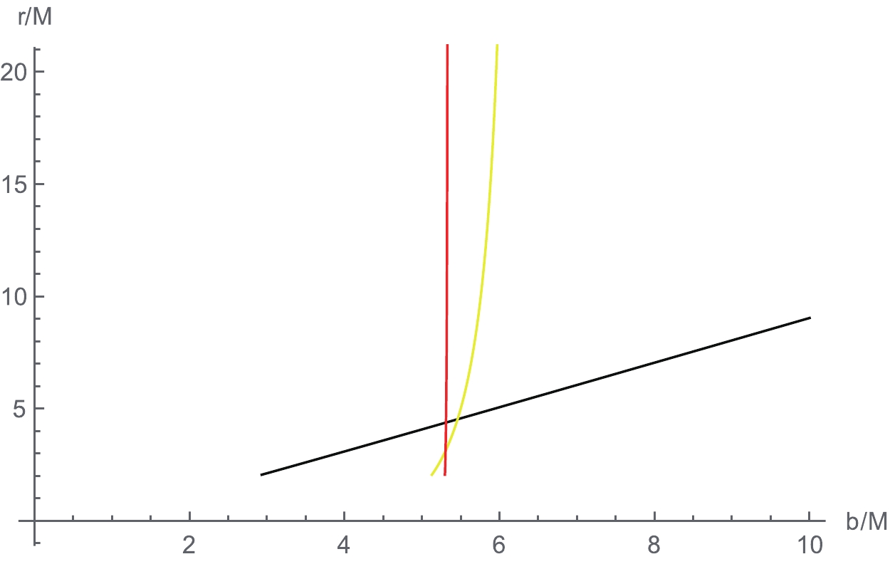
Figure 3. (color online) The first three transfer functions in a KS black hole with
$M=1, a=0.5$ . They represent the radial coordinate of the first (black), second (yellow), and third (red) intersections with the emission disk.Having obtained the transfer function, we can consider a concrete emission profile. First, we consider the case where the emission is sharply peaked at the ISCO and ends abruptly at
$r = r_{\rm isco}$ , such as$ I^{\rm em}_1(r) = \left\{ \begin{array}{ll} I^0 {\rm e}^{-(r-r_{\rm isco})}, & r>r_{\rm isco} \\ 0, & r<r_{\rm isco} \end{array} \right. \ . $

(32) Second, we consider the case where the emission is sharply peaked at the photon sphere and ends abruptly at
$ r = r_{ph} $ while quickly decaying to zero at$r = r_{\rm isco}$ , such as$ I^{\rm em}_2(r) = \left\{ \begin{array}{ll} I^0\dfrac{2-\tanh(r-r_{ph})}{2}{\rm e}^{-(r-r_{ph})}, & r>r_{ph} \\ 0, & r<r_{ph} \end{array} \right. . $

(33) Finally, we consider emission decaying gradually from the horizon to the ISCO, such as
$ I^{\rm em}_3(r) = \left\{ \begin{array}{ll} I^0\dfrac{-\tanh(r-4.5)+1}{-\tanh(r_0-4.5)+1}, & r>r_0 \\ 0, & r<r_0 \end{array} \right. . $

(34) We obtain the observed intensities
$ I^{\rm obs}(b) $ of these emission profiles with$ M = 1, a = 0.5 $ and plot the results in Fig. 4. These plots display features similar to that of a Schwarzschild black hole. The observed intensities are dominated by the direct emission, with the lensing ring emission providing only a small contribution to the total flux and the photon ring providing a negligible contribution in all cases. The radius of the main dark area, which is now called the shadow radius, is the apparent position of the edge of the emission profile resulting from direct emission. Obviously, this shadow radius is dependent on emission model. However, the photon ring always occurs at nearly$ b_c $ , and the lensing ring always occurs near$ b_c $ . Although the photon ring has highly enhanced brightness, it is barely visible in the observational appearance because it is extremely demagnified. To summarize, the significant feature of the observational appearance of thin disk emission near the black hole is the existance of a bright lensing ring near radius$ b_c $ , which is a highly demagnified image of the back of the disk.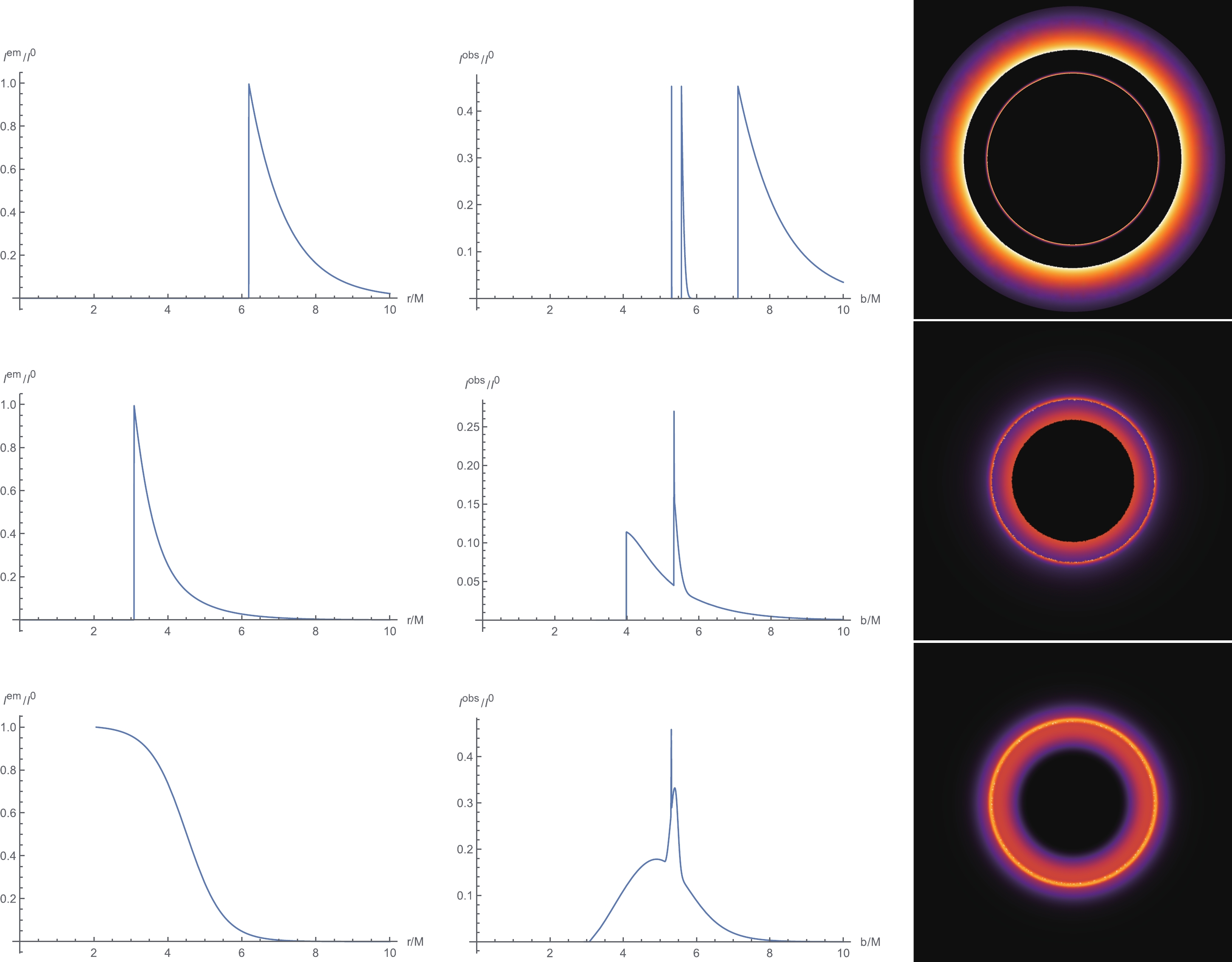
Figure 4. (color online) Observational appearance of a geometrically and optically thin disk with different emission profiles near a KS black hole with
$ M = 1, a = 0.5 $ . The left column are the plots of various emission profiles$ I^{\rm em}(r) $ . The middle column are the corresponding observed intensities$ I^{\rm obs} $ as a function of impact parameter b. The right column are the density plots of observed intensities$ I^{\rm obs}(b) $ . -
The quantum correction of a Schwarzschild black hole primarily affects the near horizon region of the metric, so it is very difficult to detect. One important feature of the near horizon region is the strong gravitational lensing effect. There exists one critical curve with impact parameter
$ b_c $ that forms a photon sphere with radius$ r_{ph} $ , and$ b_c $ gives the standard shadow radius. In this paper, we find that with quantum correction,$ r_{ph}, b_c $ violate universal inequalities (1) for an asymptotically flat black hole that satisfies the null energy condition in the framework of Einstein gravity. However, in practice, the shadow radius is dependent on the position and profile of the light source. Thus, it is unrealistic to judge the existence of quantum correction. Nevertheless, the photon ring and lensing ring are highly associated with the critical curve$ b_c $ . Because of reversed inequalities (2), we can see a larger bright lensing ring in the observational appearance of thin disk emission near the black hole compared with the classical Schwarzschild black hole. Our analysis may provide observational evidence for the quantum effect of general relativity.We conclude this paper with some future considerations. First, it is definitely interesting to investigate whether the conjecture proposed in [8, 9] is destroyed in other quantum corrected black hole models. If so, it is extremely interesting to find a general proof. Second, a novel shadow was found from a symmetric thin-shell wormhole connecting two distinct Schwarzschild spacetimes recently in [38], and one can similarly construct a thin-shell wormhole by cutting and pasting a KS black hole; thus, it is worth studying if the novel shadow exists when including the effects of quantum corrections.
Influence of quantum correction on black hole shadows, photon rings, and lensing rings
- Received Date: 2021-04-18
- Available Online: 2021-08-15
Abstract: We calculate photon sphere


 DownLoad: