


 Abstract
 HTML
HTML Reference
 Related
 PDF
PDF


-
In 2015, the LHCb collaboration observed two pentaquark or pentaquark molecule candidates,
$ P_c(4380) $ and$ P_c(4450) $ , in the$ J/\psi p $ invariant mass spectrum in$ \Lambda_b^0\to J/\psi K^- p $ decays [1]. In 2019, also in the$ J/\psi p $ invariant mass spectrum, the LHCb collaboration observed a new narrow pentaquark or pentaquark molecule candidate,$ P_c(4312) $ , and confirmed the old structure$ P_c(4450) $ , which consists of two narrow overlapping peaks,$ P_c(4440) $ and$ P_c(4457) $ [2]. There have been several possible interpretations for the quark structures of the$ P_c(4312) $ ,$ P_c(4440) $ and$ P_c(4457) $ , such as pentaquark molecular states [3-30], compact diquark-diquark-antiquark type pentaquark states or diquark-triquark type pentaquark states [31-47], color-octet-color-octet type pentaquark states [48], hadrocharmonium pentaquark states [49], etc.In Refs. [36-40], we performed comprehensive investigations of the spin-parity
$ J^P = {\dfrac{1}{2}}^\pm $ ,$ {\dfrac{3}{2}}^\pm $ and$ {\dfrac{5}{2}}^\pm $ diquark-diquark-antiquark type hidden-charm pentaquark states with QCD sum rules, by carrying out operator product expansion up to the vacuum condensates of dimension 10 in a consistent way and explicitly separating the contributions of the positive parity pentaquark states from those of the negative parity pentaquark states. We reproduced the experimental values of the masses of the$ P_c(4380) $ and$ P(4450) $ as compact pentaquark states with spin-parity$ J^P = {\dfrac{3}{2}}^- $ and$ {\dfrac{5}{2}}^+ $ , respectively. Furthermore, we obtained the lowest masses,$ 4.29 \pm 0.13\;\,\rm{GeV} $ and$ 4.30 \pm 0.13\;\,\rm{GeV} $ respectively, for the scalar-diquark–scalar-diquark-antiquark type and scalar-diquark-axialvector-diquark-antiquark type hidden-charm pentaquark states with spin-parity$ J^P = {\dfrac{1}{2}}^- $ [40], which are all consistent with the mass of the$ P_c(4312) $ observed later by the LHCb collaboration [2]. We then updated the old analysis by taking into account the vacuum condensates up to dimension 13 in a consistent way [44], and obtained flatter Borel platforms and better predictions of the masses and pole residues. The new analysis indicates that the lowest scalar-diquark–scalar-diquark-antiquark type and axialvector-diquark-axialvector-diquark-antiquark type compact hidden-charm pentaquark states with spin-parity$ J^P = {\dfrac{1}{2}}^- $ have masses$ 4.31 \pm 0.11\;\,\rm{GeV} $ and$ 4.34 \pm 0.14\;\,\rm{GeV} $ , respectively, which are all consistent with the mass of the$ P_c(4312) $ . The scalar-diquark-axialvector-diquark-antiquark type hidden-charm pentaquark state with spin-parity$ J^P = {\dfrac{1}{2}}^- $ has a mass of$ 4.45 \pm 0.11\;\,\rm{GeV} $ rather than$ 4.30 \pm 0.13\;\,\rm{GeV} $ [44].In Ref. [13], we performed detailed investigations of the
$ \bar{D}\Sigma_c $ ,$ \bar{D}\Sigma_c^* $ ,$ \bar{D}^{*}\Sigma_c $ and$ \bar{D}^{*}\Sigma_c^* $ pentaquark molecular states with QCD sum rules, by carrying out operator product expansion up to the vacuum condensates of dimension 13 in a consistent way. The theoretical predictions of the molecule masses favor assigning the$ P_c(4312) $ to be the$ \bar{D}\Sigma_c $ pentaquark molecular state with spin-parity$ J^P = {\dfrac{1}{2}}^- $ , assigning the$ P_c(4380) $ to be the$ \bar{D}\Sigma_c^* $ pentaquark molecular state with spin-parity$ J^P = {\dfrac{3}{2}}^- $ , and assigning the$ P_c(4440/4457) $ to be the$ \bar{D}^{*}\Sigma_c $ pentaquark molecular state with spin-parity$ J^P = {\dfrac{3}{2}}^- $ or the$ \bar{D}^{*}\Sigma_c^* $ pentaquark molecular state with spin-parity$ J^P = {\dfrac{5}{2}}^- $ . In the works of other theoretical groups, the$ P_c(4312) $ ,$ P_c(4380) $ ,$ P_c(4440) $ and$ P_c(4457) $ are taken as pentaquark molecular states, and their masses are studied with QCD sum rules by carrying out operator product expansion up to the vacuum condensates of dimension 8 [4, 15, 23] or 6 [11]. There are few works on the decay widths of the$ P_c(4312) $ ,$ P_c(4380) $ ,$ P_c(4440) $ and$ P_c(4457) $ . In Ref. [29] and Ref. [30], the$ P_c(4312) $ is assigned to be the pentaquark molecular state, and its two-body strong decays are studied with the QCD sum rules by carrying out operator product expansion up to the vacuum condensates of dimension 10 and 8, respectively. In Ref. [12], the$ P_c(4380) $ is assigned to be the pentaquark molecular state, and its two-body strong decays are studied with QCD sum rules by carrying out operator product expansion up to the vacuum condensates of dimension 6.It is odd that the experimental values of the masses of the
$ P_c(4312) $ ,$ P_c(4440) $ and$ P_c(4457) $ can be reproduced in the scenarios of both pentaquark states and pentaquark molecular states with the QCD sum rules. A hadron has definite quantum numbers and several Fock states. Any current with the same quantum numbers and quark structures as a Fock state in a hadron potentially couples to this hadron. In this respect, we can construct several currents to interpolate a hadron, or construct a current to interpolate several hadrons. However, we should bear in mind that a hadron has one or two main Fock states. We call a hadron a pentaquark (molecular) state if its main Fock component is of the diquark-diquark-antiquark type (color-singlet-color-singlet type), and try to choose the pertinent current to interpolate it. In the present case, the diquark-diquark-antiquark type local pentaquark current with definite quantum numbers potentially couples to a definite compact pentaquark state, though this local current can be re-arranged into a special superposition of a series of color-singlet-color-singlet type currents, which potentially couple to the pentaquark molecular states or meson-baryon two-hadron scattering states with the same quantum numbers [44]. The diquark-diquark-antiquark type pentaquark states can be taken as a special superposition of a series of color-singlet-color-singlet molecular states and embody the net effects, and vice versa.We can borrow some ideas from the nature of the light flavor scalar mesons, which are the subject of an intense and ongoing controversy in establishing the meson spectrum. The most elusive aspect is the quark configurations of the
$ f_0(980) $ and$ a_0(980) $ , which have almost degenerate masses. In the scenario of the hadronic dressing mechanism, the scalar mesons$ f_0(980) $ and$ a_0(980) $ have small or large$ q\bar{q} $ cores of typical$ q\bar{q} $ meson size, or large$ [qq]_{\bar{3}}[\bar{q}\bar{q}]_3 $ cores in the relative S-wave with some$ q\bar{q} $ components in the relative P-wave. The bare$ q\bar{q} $ or$ [qq]_{\bar{3}}[\bar{q}\bar{q}]_3 $ cores are dressed by hadronic interactions with the pseudoscalar mesons. The strong couplings to the hadronic channels or nearby thresholds enrich the pure$ q\bar{q} $ or$ [qq]_{\bar{3}}[\bar{q}\bar{q}]_3 $ states with other components, and they spend part or most of their lifetime as virtual$ K^+K^- $ or$ \bar{K}^0K^0 $ states [50-55]. The QCD sum rules indicate that the nonet scalar mesons below$ 1\,\rm{ GeV} $ are two-quark-tetraquark mixing states with large or small two-quark components [56, 57]. Without introducing mixing effects, it is difficult to reproduce the experimental values of the masses of the nonet scalar mesons below$ 1\;\rm{ GeV} $ [58, 59], and account for the decays. In summary, the QCD sum rules favor the hadronic dressing mechanism [54-57].The hadronic dressing mechanism also works in interpreting the exotic X, Y and Z states. In Ref. [60], we chose the
$ [sc]_P[\bar{s}\bar{c}]_A-[sc]_A[\bar{s}\bar{c}]_P $ type tetraquark current to study the hadronic coupling constants in the strong decays of the$ Y(4660) $ , with the QCD sum rules based on rigorous quark-hadron quality. The numerical values indicate that for the hadronic coupling constants$ |G_{Y\psi^\prime f_0}|\gg $ $ |G_{Y J/\psi f_0}| $ , which is consistent with the fact that the$ Y(4660) $ is observed in the$ \psi^\prime\pi^+\pi^- $ invariant mass distribution, and favors the$ \psi^{\prime}f_0(980) $ molecule assignment considering the decay chains$ Y(4600)\to \psi^{\prime}f_0(980) \to $ $ \psi^{\prime}\pi^+\pi^- $ [61, 62]. A similar mechanism may exist for the pentaquark states and pentaquark molecular states, i.e. the pentaquark states may have a diquark-diquark-antiquark type pentaquark core with the typical size of the$ qqq $ -type baryon states, the strong couplings to the meson-baryon pairs lead to some pentaquark molecule Fock components, the valence quarks are rearranged into color-singlet-color-singlet periphery structures, and rather a large time is spent as molecular states.In this article, we study the hadronic coupling constants of the lowest scalar-diquark-scalar-diquark-antiquark type hidden-charm pentaquark state with the QCD sum rules based on rigorous quark-hadron duality. We study its two-body strong decays and estimate the magnitude of the total decay width, examine the hadronic dressing mechanism for compact pentaquark states, and try to find a compromise between the scenarios of the pentaquark states and pentaquark molecular states.
The article is arranged as follows. In Sect. II, we illustrate how to calculate the hadronic coupling constants of the hidden-charm pentaquark states with the QCD sum rules based on rigorous quark-hadron quality. In Sect. III, we derive the QCD sum rules for the hadronic coupling constants of the lowest hidden-charm pentaquark state with spin-parity
$ J^P = {\dfrac{1}{2}}^- $ . In Sect. IV, we present the numerical results and discussion, and Sect. V is reserved for our conclusion. -
In this section, we illustrate how to calculate the hadronic coupling constants of the hidden-charm pentaquark states with the QCD sum rules. Firstly, let us write down the three-point correlation functions
$ \Pi(p,q) $ ,$ \Pi(p,q) = {\rm i}^2\int {\rm d}^4x{\rm d}^4y {\rm e}^{{\rm i}p \cdot x}{\rm e}^{{\rm i}q \cdot y}\langle 0|T\left\{J_{M}(x)J_{B}(y)\bar{J}_{P}(0)\right\}|0\rangle\, , $

(1) where
$ \bar{J}_P(0) = J_P^\dagger(0)\gamma^0 $ , the current$ J_P(0) $ interpolates the hidden-charm pentaquark state$ P_c $ , and$ J_M(x) $ and$ J_B(y) $ interpolate the traditional meson M and baryon B, respectively:$ \begin{aligned}[b] &\langle0|J_{P}(0)|P_c(p^\prime)\rangle = \lambda_{P}U(p^\prime,s) \,\, , \\ &\langle0|J_{M}(0)|M(p)\rangle = \lambda_{M} \,\, , \\ &\langle0|J_{B}(0)|B(q)\rangle = \lambda_{B}U(q,s) \,\, , \end{aligned} $

(2) where
$ \lambda_P $ ,$ \lambda_M $ and$ \lambda_{B} $ are the pole residues or decay constants, and$ U(p^\prime,s) $ and$ U(q,s) $ are the Dirac spinors.On the hadron side, we insert a complete set of intermediate hadronic states with the same quantum numbers as the current operators
$ \bar{J}_{P}(0) $ ,$ J_{M}(x) $ ,$ J_{B}(y) $ into the three-point correlation functions$ \Pi(p,q) $ , and isolate the ground state contributions of the pentaquark state$ P_c $ , traditional meson M and baryon B to obtain the hadronic representation [63, 64],$ \Pi(p,q) = -{\rm i}\lambda_{P}\lambda_{M}\lambda_{B} \frac{ \left(\!\not\!{q}+m_B \right)G_{PMB} \Gamma\left(\!\not\!\!{p}^\prime+m_P \right) }{(m_{M}^2-p^2)(m_{B}^2-q^2)(m_{P}^2-p^{\prime2})}+\cdots\, , $

(3) where
$ p^\prime = p+q $ , the$ G_{PMB} $ are the hadronic coupling constants defined by$ \langle M(p)B(q)|P_c(p^{\prime})\rangle = G_{PMB}\overline{U}(q)\Gamma U(p^\prime) \, , $

(4) and the
$ \Gamma $ are some Dirac$ \gamma $ -matrixes.In the QCD sum rules, irrespective whether they are two-point or three-point QCD sum rules, we take the quark-hadron duality to match the hadron representation with the QCD representation of the correlation functions,
$ \Pi_{H}(p,q) = \Pi_{\rm QCD}(p,q)\, , $

(5) where we add the subscripts H and
$ {\rm QCD} $ to denote the hadron side and QCD side, respectively. We expect the equality,$ \frac{1}{4}{\rm Tr}\left[\Pi_{H}(p,q)\Gamma^\prime\right] = \frac{1}{4}{\rm Tr}\left[\Pi_{\rm QCD}(p,q)\Gamma^\prime\right]\, , $

(6) survives after multiplying both sides by
$ \Gamma^\prime $ and obtaining the trace in the Dirac spinor space, where the$ \Gamma^\prime $ are some Dirac$ \gamma $ -matrixes. If we choose$ \Gamma = 1 $ and$ \Gamma^\prime = \sigma_{\mu\nu} $ , then we obtain:$ \begin{aligned}[b] &\frac{1}{4}{\rm Tr}\left[\Pi_{H}(p,q)\sigma_{\mu\nu}\right] = \Pi_{H}(p^{\prime2},p^2,q^2) \left(p_{\mu}q_{\nu}-p_{\nu}q_{\mu} \right)\, , \\ &\frac{1}{4}{\rm Tr}\left[\Pi_{\rm QCD}(p,q)\sigma_{\mu\nu}\right] = \Pi_{\rm QCD}(p^{\prime2},p^2,q^2) \left(p_{\mu}q_{\nu}-p_{\nu}q_{\mu} \right)\, , \end{aligned}$

(7) where
$ \Pi_{H}(p^{\prime2},p^2,q^2) $ and$ \Pi_{\rm QCD}(p^{\prime2},p^2,q^2) $ are the relevant components of the correlation functions$ \Pi(p,q) $ we want to study on the hadron side and QCD side, respectively. Let us write down the components of$ \Pi_{H}(p^{\prime2},p^2,q^2) $ explicitly:$ \begin{aligned}[b] \Pi_{H}(p^{\prime2},p^2,q^2) =& \frac{ \lambda_{P}\lambda_{M}\lambda_{B}G_{PMB} }{(m_{M}^2-p^2)(m_{B}^2-q^2)(m_{P}^2-p^{\prime2})}+ \frac{1}{(m_{M}^2-p^2)(m_{P}^2-p^{\prime2})} \int_{s^0_B}^\infty {\rm d}t\frac{\rho_{PB^\prime}(p^{\prime 2},p^2,t)}{t-q^2}\\ &+ \frac{1}{(m_{B}^2-q^2)(m_{P}^2-p^{\prime2})} \int_{s^0_{M}}^\infty {\rm d}t\frac{\rho_{PM^\prime}(p^{\prime 2},t,q^2)}{t-p^2} + \frac{1}{(m_{M}^2-p^{2})(m_{B}^2-q^2)} \int_{s^0_{P}}^\infty {\rm d}t\frac{\rho_{P^{\prime}M}(t,p^2,q^2)+\rho_{P^{\prime}B}(t,p^2,q^2)}{t-p^{\prime2}}+\cdots \, , \end{aligned} $ 
(8) where we introduce the four formal functions
$ \rho_{PB^\prime}(p^{\prime 2}, $ $ p^2,t) $ ,$ \rho_{PM^\prime}(p^{\prime 2},t,q^2) $ ,$ \rho_{P^{\prime}M}(t^\prime,p^2,q^2) $ and$ \rho_{P^{\prime}B}(t^\prime,p^2,q^2) $ to parameterize the complex couplings or transitions between the ground states and the higher resonances or the continuum states. In Ref. [12], the$ P_c(4380) $ is assigned to be a pentaquark molecular state, and its two-body strong decays are studied with the QCD sum rules, with the second, third and fourth terms in Eq. (8) all neglected. In Refs. [29, 30], the$ P_c(4312) $ is assigned to be a pentaquark molecular state, its two-body strong decays are studied with the QCD sum rules, and all the terms in Eq. (8) are taken into account, just as suggested in Ref. [29]. In Refs. [65, 66], the$ \Theta^+(1540) $ is assigned to be a pentaquark state, and its two-body strong decays are studied with the QCD sum rules, where the second, third or fourth term are neglected in one way or another. We should take into account all four terms in Eq. (8) to describe the transitions between the ground states and the first radial excited states in a robust way.We rewrite the correlation functions
$ \Pi_H(p^{\prime 2},p^2,q^2) $ on the hadron side as$ \Pi_{H}(p^{\prime 2},p^2,q^2) = \int_{(m_{M}+m_{B})^2}^{s_{P}^0}{\rm d}s^\prime \int_{\Delta_s^2}^{s^0_{M}}{\rm d}s \int_{\Delta_u^2}^{s^0_{B}}{\rm d}u \frac{\rho_H(s^\prime,s,u)}{(s^\prime-p^{\prime2})(s-p^2)(u-q^2)} +\int_{s^0_P}^{\infty}{\rm d}s^\prime \int_{\Delta_s^2}^{s^0_{M}}{\rm d}s \int_{\Delta_u^2}^{s^0_{B}}{\rm d}u \frac{\rho_H(s^\prime,s,u)}{(s^\prime-p^{\prime2})(s-p^2)(u-q^2)}+\cdots\, , $ 
(9) through the triple dispersion relation, where the
$ \rho_H(s^\prime,s,u) $ are the hadronic spectral densities,$ \rho_H(s^\prime,s,u) = {\lim_{\epsilon_3\to 0}}\,\,{\lim_{\epsilon_2\to 0}} \,\,{\lim_{\epsilon_1\to 0}}\,\,\frac{ {\rm Im}_{s^\prime}\, {\rm Im}_{s}\,{\rm Im}_{u}\,\Pi_H(s^\prime+{\rm i}\epsilon_3,s+{\rm i}\epsilon_2,u+{\rm i}\epsilon_1) }{\pi^3} \, , $

(10) where
$ \Delta_s^2 $ and$ \Delta_u^2 $ are the thresholds of the s and u channels, respectively, and$ s_{P}^0 $ ,$ s_{M}^0 $ ,$ s_{B}^0 $ are the continuum threshold parameters.Now we carry out the operator product expansion on the QCD side in the deep Euclidean region
$ P^2 = -p^2\gg \Lambda^2_{\rm QCD} $ and$ Q^2 = -q^2\gg \Lambda^2_{\rm QCD} $ . However, we cannot write the correlation functions$ \Pi_{\rm QCD}(p^{\prime 2},p^2,q^2) $ in the form$ \Pi_{\rm QCD}(p^{\prime 2},p^2,q^2) = \int_{(m_{M}+m_{B})^2}^{s_{P}^0}{\rm d}s^\prime \int_{\Delta_s^2}^{s^0_{M}}{\rm d}s \int_{\Delta_u^2}^{s^0_{B}}{\rm d}u \frac{\rho_{\rm QCD}(s^\prime,s,u)}{(s^\prime-p^{\prime2})(s-p^2)(u-q^2)} +\int_{s^0_P}^{\infty}{\rm d}s^\prime \int_{\Delta_s^2}^{s^0_{M}}{\rm d}s \int_{\Delta_u^2}^{s^0_{B}}{\rm d}u \frac{\rho_{\rm QCD}(s^\prime,s,u)}{(s^\prime-p^{\prime2})(s-p^2)(u-q^2)}+\cdots\, , $ 
(11) analogously through the triple dispersion relation, because the QCD spectral densities
$ \rho_{\rm QCD}(s^\prime,s,u) $ cannot exist,$ \rho_{\rm QCD}(s^\prime,s,u) = {\lim_{\epsilon_3\to 0}}\,\,{\lim_{\epsilon_2\to 0}} \,\,{\lim_{\epsilon_1\to 0}}\,\,\frac{ {\rm Im}_{s^\prime}\, {\rm Im}_{s}\,{\rm Im}_{u}\,\Pi_{\rm QCD}(s^\prime+{\rm i}\epsilon_3,s+{\rm i}\epsilon_2,u+{\rm i}\epsilon_1) }{\pi^3} = 0\, . $

(12) We have to write the correlation functions
$\Pi_{\rm QCD}(p^{\prime 2},p^2,q^2)$ in the form$ \Pi_{\rm QCD}(p^{\prime 2},p^2,q^2) = \int_{\Delta_s^2}^{s^0_{M}}{\rm d}s \int_{\Delta_u^2}^{s^0_{B}}{\rm d}u \frac{\rho_{\rm QCD}(p^{\prime2},s,u)}{(s-p^2)(u-q^2)}+\cdots\, , $

(13) through the double dispersion relation, where the
$ \rho_{\rm QCD}(p^{\prime 2},s,u) $ are the QCD spectral densities,$ \rho_{\rm QCD}(p^{\prime 2},s,u) = {\lim_{\epsilon_2\to 0}} \,\,{\lim_{\epsilon_1\to 0}}\,\,\frac{ {\rm Im}_{s}\,{\rm Im}_{u}\,\Pi_{\rm QCD}(p^{\prime 2},s+{\rm i}\epsilon_2,u+{\rm i}\epsilon_1) }{\pi^2} \, . $

(14) Henceforth, for simplicity we will write the QCD spectral densities
$ \rho_{\rm QCD}(p^{\prime 2},s,u) $ in the form$ \rho_{\rm QCD}(s,u) $ .As the duality below the three continuum threshold parameters
$ s_P^0 $ ,$ s_M^0 $ and$ s_B^0 $ cannot exist simultaneously,$ \begin{aligned}[b] &\int_{(m_{M}+m_{B})^2}^{s_{P}^0}{\rm d}s^\prime \int_{\Delta_s^2}^{s^0_{M}}{\rm d}s \int_{\Delta_u^2}^{s^0_{B}}{\rm d}u \frac{\rho_H(s^\prime,s,u)}{(s^\prime-p^{\prime2})(s-p^2)(u-q^2)}\\ \neq &\int_{(m_{M}+m_{B})^2}^{s_{P}^0}{\rm d}s^\prime \int_{\Delta_s^2}^{s^0_{M}}{\rm d}s \int_{\Delta_u^2}^{s^0_{B}}{\rm d}u \frac{\rho_{\rm QCD}(s^\prime,s,u)}{(s^\prime-p^{\prime2})(s-p^2)(u-q^2)}\, , \end{aligned} $

(15) we first carry out the formal integral over
$ {\rm d}s^\prime $ , then match the hadron side with the QCD side of the correlation functions$ \Pi(p^{\prime2},p^2,q^2) $ below the two continuum threshold parameters$ s_M^0 $ and$ s_B^0 $ simultaneously to obtain the rigorous duality [29, 60, 67-70],$ \int_{\Delta_s^2}^{s_M^0} {\rm d}s \int_{\Delta_u^2}^{s_B^0} {\rm d}u \frac{1}{(s-p^2)(u-q^2)}\left[ \int_{\Delta^2}^{\infty} {\rm d}s^\prime \frac{\rho_{H}(s^{\prime},s,u)}{s^\prime-p^{\prime2}}\right] = \int_{\Delta_s^2}^{s_M^0} {\rm d}s \int_{\Delta_u^2}^{s_B^0} {\rm d}u \frac{\rho_{\rm QCD}(s,u)}{(s-p^2)(u-q^2)}\, , \\ $

(16) where
$ \Delta^2 = (m_{M}+m_{B})^2 $ . We carry out the integral$\displaystyle\int_{\Delta^2}^{\infty} {\rm d}s^\prime \dfrac{\rho_{H}(s^{\prime},s,u)}{s^\prime-p^{\prime2}}$ according to the hadronic spectral densities in Eq. (10) to make the calculation rigorous and robust, rather than just selecting or modeling the hadron representations by hand as in Refs. [12, 65, 66]. Now let us write down the quark-hadron duality explicitly,$ \begin{aligned}[b] \int_{\Delta_s^2}^{s^0_{M}}{\rm d}s \int_{\Delta_u^2}^{s^0_{B}}{\rm d}u \frac{\rho_{\rm QCD}(s,u)}{(s-p^2)(u-q^2)} &= \int_{\Delta_s^2}^{s^0_{M}}{\rm d}s \int_{\Delta_u^2}^{s^0_{B}}{\rm d}u \int_{\Delta^2}^{\infty}{\rm d}s^\prime \frac{\rho_H(s^\prime,s,u)}{(s^\prime-p^{\prime2})(s-p^2)(u-q^2)} \\ &= \frac{\lambda_{P}\lambda_{M}\lambda_{B}G_{PMB} }{(m_{P}^2-p^{\prime2})(m_{M}^2-p^2)(m_{B}^2-q^2)} +\frac{C_{P^{\prime}M}+C_{P^{\prime}B}}{(m_{M}^2-p^{2})(m_{B}^2-q^2)} \, , \end{aligned}$ 
(17) where we introduce the parameters
$ C_{P^\prime M} $ and$ C_{P^\prime B} $ to parameterize the net effects by neglecting the dependence on the variables t,$ p^{\prime2} $ ,$ p^2 $ and$ q^2 $ ,$ \begin{aligned}[b] &C_{P^\prime M} = \int_{s^0_{P}}^\infty {\rm d}t\frac{ \rho_{P^\prime M}(t,p^2,q^2)}{t-p^{\prime2}}\, ,\\ &C_{P^\prime B} = \int_{s^0_{P}}^\infty {\rm d}t\frac{ \rho_{P^\prime B}(t,p^2,q^2)}{t-p^{\prime2}}\, .\end{aligned} $

(18) From Eq. (17), we can see that the duality below the continuum threshold parameters
$ s_M^0 $ and$ s_B^0 $ is rigorous.In Eqs. (16)-(17), the continuum threshold parameters
$ s^0_{M} $ and$ s^0_{B} $ appear in both the hadron side and QCD side of the correlation functions. As the spectroscopy of the traditional mesons and baryons is known much better than that of the pentaquark states, even though the pentaquark states have not been established yet, we can consult the experimental data from the Particle Data Group and the theoretical predictions from the two-point QCD sum rules to choose suitable continuum threshold parameters$ s^0_{M} $ and$ s^0_{B} $ , which should be large enough to fully include the contributions of the ground states, but small enough to exclude the contaminations of higher excited states and continuum states.In the two-point QCD sum rules for the conventional baryons B and mesons M,
$ \lambda_{i}^2\exp\left(-\tau m_i^2 \right) = \int_{\Delta_i^2}^{s_i^0} {\rm d}s \,\rho_{\rm QCD}(s)\exp\left( -\tau s\right)\, , $

(19) $ m_i^2 = \frac{-\dfrac{\rm d}{{\rm d}\tau}\displaystyle\int_{\Delta_i^2}^{s_i^0} {\rm d}s \,\rho_{\rm QCD}(s)\exp\left( -\tau s\right)}{\displaystyle\int_{\Delta_i^2}^{s_i^0} {\rm d}s \,\rho_{\rm QCD}(s)\exp\left( -\tau s\right)}\, , $

(20) where
$ i = B $ , M,$ \tau = \dfrac{1}{T^2} $ , and$ T^2 $ is the Borel parameter. The predicted masses$ m_{B/M} $ and pole residues$ \lambda_{B/M} $ vary with the continuum threshold parameters$ s^0_{B/M} $ . In calculation, we observe that the uncertainties of the continuum threshold parameters,$ s^0_{i} \to s^0_{i}+\delta s^0_{i} $ , can lead to uncertainties of the masses and pole residues,$ m_{i}\to m_{i}+ $ $ \delta m_{i} $ and$ \lambda_{i}\to \lambda_{i}+\delta\lambda_{i} $ , with the relation$ \dfrac{\delta\lambda_{i}}{\lambda_{i}}\gg \dfrac{\delta m_{i}}{m_{i}} $ . In Eqs. (16)-(17), and in other three-point QCD sum rules for the hadronic coupling constants, we usually take the physical masses$ m_{P/B/M} $ as input parameters and neglect the small uncertainties. Furthermore, we can factorize out the pole residues$ \lambda_{B/M} $ from the unknown functions$ C_{P^\prime M} = \lambda_{M}\lambda_{B}\widetilde{C}_{P^\prime M} $ and$ C_{P^\prime B} = \lambda_{M}\lambda_{B}\widetilde{C}_{P^\prime B} $ ,$ \int_{\Delta_s^2}^{s^0_{M}}{\rm d}s \int_{\Delta_u^2}^{s^0_{B}}{\rm d}u \frac{\rho_{\rm QCD}(s,u)}{(s-p^2)(u-q^2)} = \lambda_{M}\lambda_{B}\left[ \frac{\lambda_{P}G_{PMB} }{(m_{P}^2-p^{\prime2})(m_{M}^2-p^2)(m_{B}^2-q^2)}+ \frac{\widetilde{C}_{P^{\prime}M}+\widetilde{C}_{P^{\prime}B}}{(m_{M}^2-p^{2})(m_{B}^2-q^2)}\right] \, . $ 
(21) The uncertainties from the continuum threshold parameters
$ s^0_{M/B} $ can be approximately absorbed into the pole residues; considering the integrals$ {\rm d}s $ and$ {\rm d}u $ on both sides of Eqs. (16)-(17), the net effects due to$ \delta s^0_{B/M} $ are tiny. We choose the ideal values of the continuum threshold parameters$ s^0_{M/B} $ , which happen to reproduce the experimental values of the masses$ m_{M/B} $ approximately, and neglect the uncertainties for simplicity.In fact, the QCD spectral densities
$ \rho_{\rm QCD}(s,u) $ cannot be factorized out as$ \rho_{\rm QCD}(s)\,\rho_{\rm QCD}(u) $ , and the continuum threshold parameters$ s_0 $ and$ u_0 $ are not necessarily those obtained from the two-point QCD sum rules. We can take the values obtained from the two-point QCD sum rules as a guide, and vary$ s_0 $ and$ u_0 $ to search for the best parameters in the three-point QCD sum rules via trial and error. In calculation, we observe that the deviations$ \delta s_0 $ and$ \delta u_0 $ can also be compensated by variations of the parameters$ \widetilde{C}_{P^{\prime}M} $ and$ \widetilde{C}_{P^{\prime}B} $ , if we fix the values of the pole residues$ \lambda_{M} $ and$ \lambda_{B} $ . The continuum threshold parameters$ s_0 $ and$ u_0 $ from the two-point QCD sum rules work well in the three-point QCD sum rules.In numerical calculations, we can take the unknown functions
$ C_{P^\prime M} $ and$ C_{P^\prime B} $ as free parameters, and choose suitable values to account for the contaminations of the higher resonances and continuum states in the$ s^\prime $ channel to obtain the stable QCD sum rules. The parameters$ C_{P^\prime M} $ and$ C_{P^\prime B} $ are not necessarily constants. They may depend on the Borel parameters, as there are complex interactions or transitions between the ground states and the higher resonances or continuum states. After the double Borel transform, some net Borel parameter dependence may appear.If M is a charmonium or bottomonium state and B is a light flavor baryon state, we set
$ p^{\prime2} = p^2 $ and perform the double Borel transform in regard to the variables$ P^2 = -p^2 $ and$ Q^2 = -q^2 $ respectively to obtain the QCD sum rules,$ \begin{aligned}[b] &\frac{\lambda_{P}\lambda_{M}\lambda_{B}G_{PMB}}{m_{P}^2-m_{M}^2} \left[ \exp\left(-\frac{m_{M}^2}{T_1^2} \right)-\exp\left(-\frac{m_{P}^2}{T_1^2} \right)\right]\exp\left(-\frac{m_{B}^2}{T_2^2} \right) +\left(C_{P^{\prime}M}+C_{P^{\prime}B}\right) \exp\left(-\frac{m_{M}^2}{T_1^2} -\frac{m_{B}^2}{T_2^2} \right)\\=& \int_{\Delta_s^2}^{s_M^0} {\rm d}s \int_{\Delta_u^2}^{s_B^0} {\rm d}u\, \rho_{\rm QCD}(s,u)\exp\left(-\frac{s}{T_1^2} -\frac{u}{T_2^2} \right)\, ,\end{aligned} $ 
(22) where
$ T_1^2 $ and$ T_2^2 $ are the Borel parameters. On the other hand, if M is a heavy meson and B is a heavy baryon state, we set$ p^{\prime2} = 4q^2 $ and perform the double Borel transform in regard to the variables$ P^2 = -p^2 $ and$ Q^2 = -q^2 $ respectively to obtain the QCD sum rules,$ \begin{aligned}[b] &\frac{\lambda_{P}\lambda_{M}\lambda_{B}G_{PMB}}{4\left(\widetilde{m}_{P}^2-m_{B}^2\right)} \left[ \exp\left(-\frac{m_{B}^2}{T_2^2} \right)-\exp\left(-\frac{\widetilde{m}_{P}^2}{T_2^2} \right)\right]\exp\left(-\frac{m_{M}^2}{T_1^2} \right) + \left(C_{P^{\prime}M}+C_{P^{\prime}B}\right) \exp\left(-\frac{m_{B}^2}{T_2^2} -\frac{m_{M}^2}{T_1^2} \right) \\ =& \int_{\Delta_s^2}^{s_M^0} {\rm d}s \int_{\Delta_u^2}^{s_B^0} {\rm d}u\, \rho_{\rm QCD}(s,u)\exp\left(-\frac{s}{T_1^2} -\frac{u}{T_2^2} \right)\, , \end{aligned} $ 
(23) where
$ \widetilde{m}_P^2 = \dfrac{m_P^2}{4} $ .In the QCD sum rules in Eqs. (22)-(23), the Borel parameters
$ T_1^2 $ and$ T_2^2 $ are independent parameters, and the intervals of dimensions of the vacuum condensates are small. In calculations, we can set$ T_1^2 = T_2^2 = T^2 $ to obtain much larger intervals of dimensions of the vacuum condensates, and therefore much more stable QCD sum rules and much better accuracy of the predictions. -
In the following, we write down the three-point correlation functions
$ \Pi(p,q) $ and$ \Pi_{\mu}(p,q) $ in the QCD sum rules:$ \Pi(p,q) \!=\! {\rm i}^2\!\!\int \!\! {\rm d}^4x{\rm d}^4y {\rm e}^{{\rm i}p \cdot x}{\rm e}^{{\rm i}q \cdot y} \langle0|T\left\{J_M(x)J_B(y)\bar{J}_P(0)\right\}|0\rangle \, , $

(24) $ \Pi_\mu(p,q) \!=\! {\rm i}^2\!\!\int\!\! {\rm d}^4x{\rm d}^4y {\rm e}^{{\rm i}p \cdot x}{\rm e}^{{\rm i}q \cdot y} \langle0|T\left\{J_\mu(x)J_N(y)\bar{J}_P(0)\right\}|0\rangle \, , $

(25) where
$ J_M(x) = J_{\eta_c}(x) $ ,$ J_{\bar{D}^0}(x) $ ,$ J_{D^-}(x) $ ,$ J_B(y) = J_{\Lambda_c^+}(y) $ ,$ J_{\Sigma_c^{++}}(y) $ ,$ J_{\Sigma_c^+}(y) $ , and$ J_N(y) $ :$ \begin{aligned}[b] &J_{\eta_c}(x) = \bar{c}(x){\rm i}\gamma_5 c(x)\, ,\\ &J_{\bar{D}^0}(x) = \bar{c}(x){\rm i}\gamma_5 u(x)\, ,\\ &J_{D^-}(x) = \bar{c}(x){\rm i}\gamma_5 d(x)\, ,\\ &J_\mu(x) = \bar{c}(x) \gamma_\mu c(x)\, , \end{aligned} $

(26) $ \begin{aligned}[b] &J_{\Lambda_c^+}(y) = \varepsilon^{ijk} u^T_i(y) C\gamma_5 d_j(y)\, c_{k}(y) \, , \\ &J_{\Sigma_c^{++}}(y) = \varepsilon^{ijk} u^T_i(y) C\gamma_\alpha u_j(y)\, \gamma^\alpha\gamma_5 c_{k}(y) \, , \\ &J_{\Sigma_c^+}(y) = \varepsilon^{ijk} u^T_i(y) C\gamma_\alpha d_j(y)\, \gamma^\alpha\gamma_5 c_{k}(y) \, , \\ &J_N(y) = \varepsilon^{ijk} u^T_i(y) C\gamma_\alpha u_j(y)\, \gamma^\alpha\gamma_5 d_{k}(y) \, , \end{aligned} $

(27) $ J_P(0) \!=\! \varepsilon^{ila}\! \varepsilon^{ijk}\!\varepsilon^{lmn} u^T_j(0) C\gamma_5 d_k(0)\,u^T_m(0) C\gamma_5 c_n(0)\, C\bar{c}^{T}_{a}(0) \, , $

(28) with a, i, j,
$ \cdots $ being color indices. We choose the quark currents$ J_{\eta_c}(x) $ ,$ J_{\bar{D}^0}(x) $ ,$ J_{D^-}(x) $ ,$ J_\mu(x) $ ,$ J_{\Lambda_c^+}(y) $ ,$ J_{\Sigma_c^{++}}(y) $ ,$ J_{\Sigma_c^+}(y) $ ,$ J_N(y) $ and$ J_P(0) $ to interpolate the hadrons$ \eta_c $ ,$ \bar{D}^0 $ ,$ D^- $ ,$ J/\psi $ ,$ \Lambda_c^+ $ ,$ \Sigma_c^{++} $ ,$ \Sigma_c^+ $ , p and$ P_c $ , respectively. Henceforth we will write the proton as N instead of p to avoid confusion with the four-momentum$ p_\mu $ .On the hadron side, we insert a complete set of intermediate hadron states with the same quantum numbers as the current operators
$ J_{\eta_c}(x) $ ,$ J_{\bar{D}^0}(x) $ ,$ J_{D^-}(x) $ ,$ J_\mu(x) $ ,$ J_{\Lambda_c^+}(y) $ ,$ J_{\Sigma_c^+}(y) $ ,$ J_{\Sigma_c^{++}}(y) $ ,$ J_N(y) $ and$ \bar{J}_P(0) $ into the correlation functions$ \Pi(p,q) $ and$ \Pi_{\mu}(p,q) $ respectively to obtain the hadronic representation [63, 64], then we isolate all the ground state contributions and write them down explicitly:$ \Pi_{P\eta_cN}(p,q) = \frac{f_{\eta_c}m_{\eta_c}^2\lambda_P\lambda_N}{2m_c}\frac{-{\rm i} \left(\!\not\!{q}+m_N \right)\left( \!\not\!\!{p}^\prime+m_P \right)}{\left(m_P^2-p^{\prime2}\right)\left(m_{\eta_c}^2-p^{2}\right)\left(m_{N}^2-q^{2}\right)}G_{P\eta_cN}+\cdots\, , $ 
(29) $ \Pi_{P\bar{D}^0\Lambda_c^+}(p,q) = \frac{f_{D}m_{D}^2\lambda_P\lambda_{\Lambda_c}}{m_c}\frac{-{\rm i} \left(\!\not\!{q}+m_{\Lambda_c} \right)\left( \!\not\!{p}^\prime+m_P \right)}{\left(m_P^2-p^{\prime2}\right)\left(m_{D}^2-p^{2}\right)\left(m_{\Lambda_c}^2-q^{2}\right)}G_{P\bar{D}^0\Lambda_c^+}+\cdots\, , $

(30) $ \Pi_{P\bar{D}^0\Sigma_c^+}(p,q) = \frac{f_{D}m_{D}^2\lambda_P\lambda_{\Sigma^+_c}}{m_c}\frac{-{\rm i} \left(\!\not\!{q}+m_{\Sigma_c} \right)\left( \!\not\!\!{p}^\prime+m_P \right)}{\left(m_P^2-p^{\prime2}\right)\left(m_{D}^2-p^{2}\right)\left(m_{\Sigma_c}^2-q^{2}\right)}G_{P\bar{D}^0\Sigma_c^+}+\cdots\, , $

(31) $ \Pi_{P D^-\Sigma_c^{++}}(p,q) = \frac{f_{D}m_{D}^2\lambda_P\lambda_{\Sigma^{++}_c}}{m_c}\frac{-{\rm i} \left(\!\not\!{q}+m_{\Sigma_c} \right)\left( \!\not\!\!{p}^\prime+m_P \right)}{\left(m_P^2-p^{\prime2}\right)\left(m_{D}^2-p^{2}\right)\left(m_{\Sigma_c}^2-q^{2}\right)}G_{P D^-\Sigma_c^{++}}+\cdots\, , $

(32) $ \Pi_\mu(p,q) = f_{J/\psi}m_{J/\psi}\lambda_P\lambda_N\dfrac{- \left(\!\not\!{q}+m_N \right)\left( G_V\gamma^\alpha-{\rm i}\dfrac{G_T}{m_P+m_N}\sigma^{\alpha\beta}p_\beta\right)\gamma_5\left( \!\not\!\!{p}^\prime+m_P \right)}{\left(m_P^2-p^{\prime2}\right)\left(m_{J/\psi}^2-p^{2}\right)\left(m_{N}^2-q^{2}\right)}\left(-g_{\mu\alpha}+\dfrac{p_{\mu}p_{\alpha}}{p^2} \right)+\cdots\, ,$

(33) where we introduce the subscripts
$ P\eta_cN $ ,$ P\bar{D}^0\Lambda_c^+ $ ,$ P\bar{D}^0\Sigma_c^+ $ and$ P D^{-}\Sigma_c^{++} $ in the correlation functions$ \Pi(p,q) $ to distinguish the corresponding hadronic coupling constants, and we take the standard definitions for the pole residues or decay constants$ \lambda_{P} $ ,$ \lambda_{N} $ ,$ \lambda_{\Lambda_c} $ ,$ \lambda_{\Sigma_c} $ ,$ f_{\eta_c} $ ,$ f_{D} $ ,$ f_{J/\psi} $ :$ \begin{aligned}[b] &\langle 0| J (0)|P_{c}(p^\prime)\rangle = \lambda_{P} U(p^\prime,s)\, ,\;\; \langle 0| J_{N} (0)|N(q)\rangle = \lambda_{N} U(q,s) \, , \\ &\langle 0| J_{\Lambda_c} (0)|\Lambda_c(q)\rangle = \lambda_{\Lambda_c} U(q,s) \, , \;\; \langle 0| J_{\Sigma_c} (0)|\Sigma_c(q)\rangle = \lambda_{\Sigma_c} U(q,s) \, , \\ &\langle 0| J_{\eta_c} (0)|\eta_c(p)\rangle = \frac{f_{\eta_c}m_{\eta_c}^2}{2m_c} \, , \;\;\langle 0| J_{D} (0)|D(p)\rangle = \frac{f_{D}m_{D}^2}{m_c} \, , \\ &\langle 0| J_{\mu} (0)|J/\psi(p)\rangle = f_{J/\psi}m_{J/\psi}\varepsilon_\mu(p,s) \, , \end{aligned} $

(34) and the hadronic coupling constants
$ G_{P\eta_cN} $ ,$ G_{P\bar{D}^0\Lambda_c^+} $ ,$ G_{P\bar{D}^0\Sigma_c^+} $ ,$ G_{PD^-\Sigma_c^{++}} $ ,$ G_V $ and$ G_T $ :$ \begin{aligned}[b] &\langle\eta_c(p)N(q)|P_c(p^\prime)\rangle = G_{P\eta_cN}\,\overline{U}(q)U(p^\prime)\, ,\\ &\langle \bar{D}^0(p)\Lambda_c^+(q)|P_c(p^\prime)\rangle = G_{P\bar{D}^0\Lambda_c^+}\,\overline{U}(q)U(p^\prime)\, ,\\ &\langle \bar{D}^0(p)\Sigma_c^+(q)|P_c(p^\prime)\rangle = G_{P\bar{D}^0\Sigma_c^+}\,\overline{U}(q)U(p^\prime)\, ,\\ &\langle D^-(p)\Sigma_c^{++}(q)|P_c(p^\prime)\rangle = G_{PD^-\Sigma_c^{++}}\,\overline{U}(q)U(p^\prime)\, ,\\ &\langle J/\psi(p)N(q)|P_c(p^\prime)\rangle = -{\rm i}\overline{U}(q)\varepsilon^*_\alpha\Biggr( G_V\gamma^\alpha\\ &\qquad\qquad -{\rm i}\frac{G_T}{m_P+m_N}\sigma^{\alpha\beta}p_\beta\Biggr)\gamma_5U(p^\prime)\, ,\end{aligned} $

(35) where
$ U(p^\prime,s) $ ,$ U(p,s) $ and$ U(q,s) $ are the Dirac spinors, and$ \varepsilon_\mu $ is the polarization vector of the$ J/\psi $ .In this article, we choose
$ \Gamma^\prime = \sigma_{\mu\nu} $ ,$ \gamma_5\!\not\!{z} $ ,$ \gamma_5 $ in Eq. (6), and obtain the traces in Dirac spinor space:$ \begin{aligned}[b]&\frac{1}{4}{\rm Tr}\left[\Pi_{H}(p,q)\sigma_{\mu\nu}\right] = \Pi_H(p^{\prime2},p^2,q^2) \,\left(p_\mu q_\nu-q_\mu p_\nu \right)+\cdots\, , \\ &\frac{1}{4}{\rm Tr}\left[\Pi_\mu^{H}(p,q)\gamma_5\!\not\!{z} \right] = \Pi_H^1(p^{\prime2},p^2,q^2)\, q_\mu p\cdot z+\cdots\, ,\\ &\frac{1}{4}{\rm Tr}\left[\Pi_\mu^{H}(p,q)\gamma_5 \right] = \Pi_H^2(p^{\prime2},p^2,q^2)\, q_\mu +\cdots\, . \end{aligned} $

(36) We choose the tensor structures
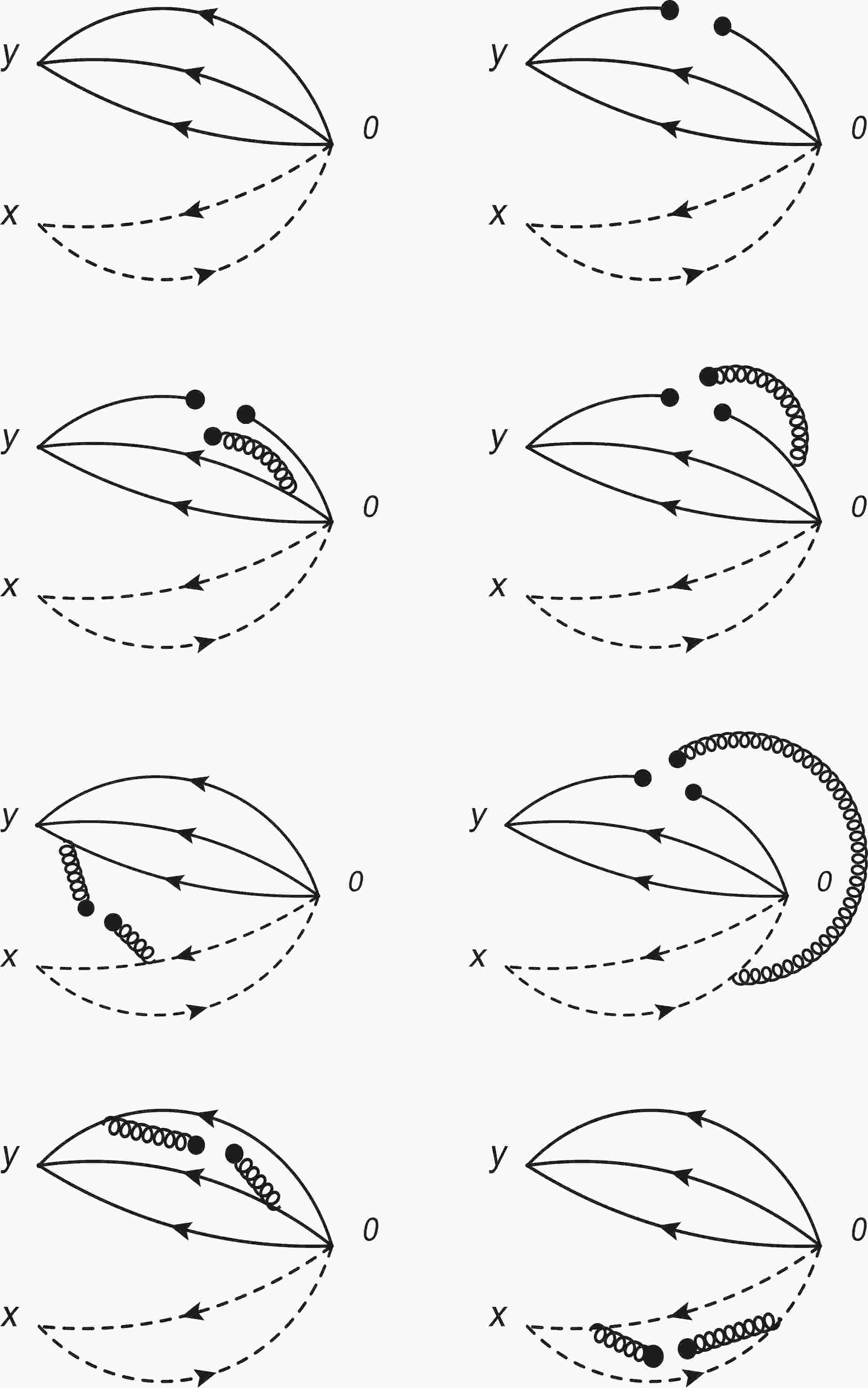
$ p_\mu q_\nu-q_\mu p_\nu $ ,$ q_\mu p\cdot z $ and$ q_\mu $ to study the hadronic coupling constants, where$ z_\mu $ is an arbitrary four-vector we introduce to select the pertinent Dirac structures. For simplicity, we neglect the explicit expressions for the correlation functions$ \Pi_H(p^{\prime2},p^2,q^2) $ ,$ \Pi_H^1(p^{\prime2},p^2,q^2) $ and$ \Pi_H^2(p^{\prime2},p^2,q^2) $ on the hadron side.On the QCD side of the correlation functions, we carry out the operator product expansion up to the vacuum condensates of dimension-10. The interval of the vacuum condensates is large enough to obtain stable QCD sum rules in the case of a single Borel parameter. The relevant Feynman diagrams are shown explicitly in Fig. 1. Moreover, we assume vacuum saturation for the higher-dimensional vacuum condensates. As the vacuum condensates are vacuum expectations of the quark-gluon operators of dimension n, we take the truncations
$ \mathcal{O}( \alpha_s^{k}) $ with$n\leqslant 10$ and$k\leqslant 1$ in a consistent way, and write (components of) the correlation functions$ \Pi_{\rm QCD}(p^{\prime 2}, $ $ p^2,q^2) $ as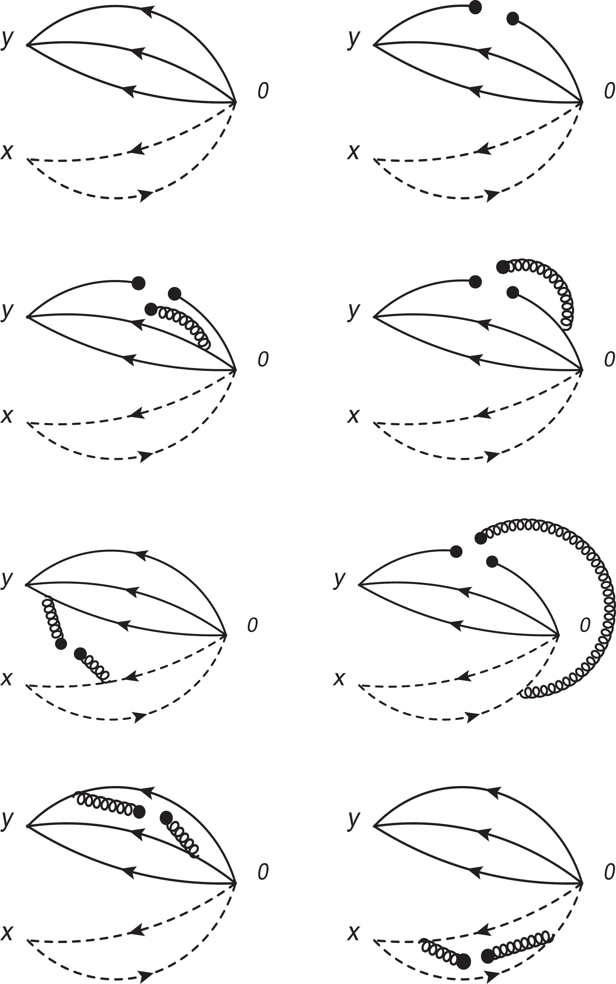
Figure 1. Feynman diagrams contributing to the two-body strong decays. Other diagrams obtained by interchanging of the light quark lines (solid lines) or heavy quark lines (dashed lines) are implied.
$ \Pi_{\rm QCD}(p^{\prime 2},p^2,q^2) = \int_{\Delta_s^2}^{s^0_{M}}{\rm d}s \int_{\Delta_u^2}^{s^0_{B}}{\rm d}u \frac{\rho_{\rm QCD}(s,u)}{(s-p^2)(u-q^2)}+\cdots\, , $

(37) through the double dispersion relation, where for simplicity the
$ \Pi_{\rm QCD}(p^{\prime 2}, $ $ p^2,q^2) $ collectively represent the corresponding correlation functions of the$ \Pi_H(p^{\prime2},p^2,q^2) $ ,$ \Pi_H^1(p^{\prime2},p^2,q^2) $ and$ \Pi_H^2(p^{\prime2},p^2,q^2) $ on the QCD side.Here we take a short digression to discuss the vacuum saturation in performing the operator product expansion. In the original works on this topic, Shifman, Vainshtein and Zakharov took the factorization hypothesis for the higher dimensional vacuum condensates for two reasons [63]. One is the rather large value of the quark condensate
$ \langle\bar{q}q\rangle $ , and the other is the duality between the quark and physical states, which implies that counting both the quark and physical states may well become a double counting since they reproduce each other [63].In the QCD sum rules for the traditional mesons, we always introduce a parameter
$ \kappa $ to parameterize the deviation from the factorization hypothesis by hand. For example, in the case of the four-quark condensate,$ \langle\bar{q}q\rangle^2 \to \kappa\langle\bar{q}q\rangle^2 $ [71-73]. As the$ \langle\bar{q}q\rangle^2 $ is always companied by the fine-structure constant$ \alpha_s = \dfrac{g_s^2}{4\pi} $ , and plays only a minor role, any deviation from$ \kappa = 1 $ , for example,$ \kappa = 2\sim 3 $ , cannot make much difference, though$ \kappa>1 $ can lead to better QCD sum rules in some cases. In fact, the vacuum saturation works well in the large$ N_c $ limit [74].On the other hand, in the QCD sum rules for the tetraquark, pentaquark and hexaquark (or molecular) states, the four-quark condensate plays an important role. A large value, for example,
$ \kappa = 2 $ , can destroy the platforms in the QCD sum rules for the current$ J_{c\bar{c}}(x) $ in Ref. [75]. Furthermore, in calculation, we observe that the optimal value is$ \kappa = 1 $ , and vacuum saturation works well in the QCD sum rules for the multiquark states.Up to now, all the multiquark states have been studied with QCD sum rules by tacitly assuming vacuum saturation for the higher dimensional vacuum condensates in performing the operator product expansion, except for some cases where the parameter
$ \kappa $ is introduced for the sake of fine-tuning. The true values (also the next-to-leading-order perturbative corrections) of the higher-dimensional vacuum condensates, even the four-quark condensates$ \langle \bar{q}\Gamma q \bar{q}\Gamma^\prime q\rangle $ , where the$ \Gamma $ and$ \Gamma^\prime $ stand for the Dirac$ \gamma $ -matrixes, remain unknown or poorly known, and we cannot obtain robust estimations of the effects beyond vacuum saturation.Now we come back to the correlation functions
$ \Pi(p^{\prime 2},p^2,q^2) $ , and integrate over$ {\rm d}s^\prime $ first on the hadron side, using Eqs. (16)-(17), then match the hadron side with the QCD side of the correlation functions$ \Pi(p^{\prime 2},p^2,q^2) $ to obtain the rigorous duality. We then write down the quark-hadron duality explicitly:$ \int_{4m_c^2}^{s^0_{\eta_c}}{\rm d}s \int_{0}^{s^0_{N}}{\rm d}u \frac{\rho^{\eta_cN}_{\rm QCD}(s,u)}{(s-p^2)(u-q^2)} = \frac{f_{\eta_c}m_{\eta_c}^2\lambda_P\lambda_N}{2m_c}\frac{G_{P\eta_cN}}{\left(m_P^2-p^{\prime2}\right)\left(m_{\eta_c}^2-p^{2}\right)\left(m_{N}^2-q^{2}\right)} +\frac{C_{P^{\prime}\eta_c}+C_{P^{\prime}N}}{(m_{\eta_c}^2-p^{2})(m_{N}^2-q^2)} \, , $ 
(38) $ \int_{m_c^2}^{s^0_{D}}{\rm d}s \int_{m_c^2}^{s^0_{\Lambda_c}}{\rm d}u \frac{\rho^{\bar{D}^0\Lambda^+_c}_{\rm QCD}(s,u)}{(s-p^2)(u-q^2)} = \frac{f_{D}m_{D}^2\lambda_P\lambda_{\Lambda_c}}{m_c}\frac{G_{P\bar{D}^0\Lambda^+_c}}{\left(m_P^2-p^{\prime2}\right)\left(m_{D}^2-p^{2}\right)\left(m_{\Lambda_c}^2-q^{2}\right)} +\frac{C_{P^{\prime}\bar{D}^0}+C_{P^{\prime}\Lambda^+_c}}{(m_{D}^2-p^{2})(m_{\Lambda_c}^2-q^2)} \, , $

(39) $ \int_{m_c^2}^{s^0_{D}}{\rm d}s \int_{m_c^2}^{s^0_{\Sigma_c}}{\rm d}u \frac{\rho^{\bar{D}^0\Sigma^+_c}_{\rm QCD}(s,u)}{(s-p^2)(u-q^2)} = \frac{f_{D}m_{D}^2\lambda_P\lambda_{\Sigma^+_c}}{m_c}\frac{G_{P\bar{D}^0\Sigma^+_c}}{\left(m_P^2-p^{\prime2}\right)\left(m_{D}^2-p^{2}\right)\left(m_{\Sigma_c}^2-q^{2}\right)} +\frac{C_{P^{\prime}\bar{D}^0}+C_{P^{\prime}\Sigma^+_c}}{(m_{D}^2-p^{2})(m_{\Sigma_c}^2-q^2)} \, ,$

(40) $ \int_{m_c^2}^{s^0_{D}}{\rm d}s \int_{m_c^2}^{s^0_{\Sigma_c}}{\rm d}u \frac{\rho^{D^-\Sigma^{++}_c}_{\rm QCD}(s,u)}{(s-p^2)(u-q^2)} = \frac{f_{D}m_{D}^2\lambda_P\lambda_{\Sigma^{++}_c}}{m_c}\frac{G_{PD^-\Sigma^{++}_c}}{\left(m_P^2-p^{\prime2}\right)\left(m_{D}^2-p^{2}\right)\left(m_{\Sigma_c}^2-q^{2}\right)} +\frac{C_{P^{\prime}D^-}+C_{P^{\prime}\Sigma^{++}_c}}{(m_{D}^2-p^{2})(m_{\Sigma_c}^2-q^2)} \, ,$

(41) $ \int_{4m_c^2}^{s^0_{J/\psi}}{\rm d}s \int_{0}^{s^0_{N}}{\rm d}u \frac{\rho^{J/\psi N,1}_{\rm QCD}(s,u)}{(s-p^2)(u-q^2)} = f_{J/\psi}m_{J/\psi}\lambda_P\lambda_N \frac{G_T-G_V}{\left(m_P^2-p^{\prime2}\right)\left(m_{J/\psi}^2-p^{2}\right)\left(m_{N}^2-q^{2}\right)} +\frac{C_{P^{\prime}J/\psi,1}+C_{P^{\prime}N,1}}{(m_{J/\psi}^2-p^{2})(m_{N}^2-q^2)} \, , $

(42) $ \int_{4m_c^2}^{s^0_{J/\psi}}{\rm d}s \int_{0}^{s^0_{N}}{\rm d}u \frac{\rho^{J/\psi N,2}_{\rm QCD}(s,u)}{(s-p^2)(u-q^2)} = f_{J/\psi}m_{J/\psi}\lambda_P\lambda_N \frac{\left(m_P-m_N\right)G_V-G_T\frac{m_{J/\psi}^2}{m_P+m_N}}{\left(m_P^2-p^{\prime2}\right)\left(m_{J/\psi}^2-p^{2}\right)\left(m_{N}^2-q^{2}\right)} +\frac{C_{P^{\prime}J/\psi,2}+C_{P^{\prime}N,2}}{(m_{J/\psi}^2-p^{2})(m_{N}^2-q^2)} \, , $

(43) where the parameters
$ C_{P^{\prime}\eta_c}+C_{P^{\prime}N} $ ,$ C_{P^{\prime}\bar{D}^0}+C_{P^{\prime}\Lambda^+_c} $ ,$ C_{P^{\prime}\bar{D}^0}+ $ $ C_{P^{\prime}\Sigma^{+}_c} $ ,$ C_{P^{\prime}D^{-}}+C_{P^{\prime}\Sigma^{++}_c} $ ,$ C_{P^{\prime}J/\psi,1}+C_{P^{\prime}N,1} $ and$ C_{P^{\prime}J/\psi,2}+C_{P^{\prime}N,2} $ are defined according to Eq. (18).We perform a double Borel transform with respect to the variables
$ P^2 = -p^2 $ and$ Q^2 = -q^2 $ respectively, using Eqs. (22)-(23) to obtain the QCD sum rules:$ \begin{aligned}[b]&\frac{f_{\eta_c}m_{\eta_c}^2\lambda_P\lambda_N}{2m_c} \frac{G_{P\eta_cN}}{m_{P}^2-m_{\eta_c}^2} \left[ \exp\left(-\frac{m_{\eta_c}^2}{T_1^2} \right)-\exp\left(-\frac{m_{P}^2}{T_1^2} \right)\right]\exp\left(-\frac{m_{N}^2}{T_2^2} \right) + \left(C_{P^{\prime}\eta_c}+C_{P^{\prime}N}\right) \exp\left(-\frac{m_{\eta_c}^2}{T_1^2} -\frac{m_{N}^2}{T_2^2} \right) \\ =&\int_{4m_c^2}^{s_{\eta_c}^0} {\rm d}s \int_{0}^{s_N^0} {\rm d}u\, \rho^{\eta_cN}_{\rm QCD}(s,u)\exp\left(-\frac{s}{T_1^2} -\frac{u}{T_2^2} \right)\, , \end{aligned}$

(44) $ \begin{aligned}[b]&\frac{f_{D}m_{D}^2\lambda_P\lambda_{\Lambda_c}}{4m_c} \frac{G_{P\bar{D}^0\Lambda_c^+}}{\widetilde{m}_{P}^2-m_{\Lambda_c}^2} \left[ \exp\left(-\frac{m_{\Lambda_c}^2}{T_2^2} \right)-\exp\left(-\frac{\widetilde{m}_{P}^2}{T_2^2} \right)\right]\exp\left(-\frac{m_{D}^2}{T_1^2} \right) + \left(C_{P^{\prime}\bar{D}^0}+C_{P^{\prime}\Lambda_c^+}\right) \exp\left(-\frac{m_{\Lambda_c}^2}{T_2^2} -\frac{m_{D}^2}{T_1^2} \right)\\ =&\int_{m_c^2}^{s_{D}^0} {\rm d}s \int_{m_c^2}^{s_{\Lambda_c}^0} {\rm d}u\, \rho^{\bar{D}^0\Lambda_c^+}_{\rm QCD}(s,u)\exp\left(-\frac{s}{T_1^2} -\frac{u}{T_2^2} \right)\, ,\end{aligned} $

(45) $ \begin{aligned}[b]&\frac{f_{D}m_{D}^2\lambda_P\lambda_{\Sigma^+_c}}{4m_c} \frac{G_{P\bar{D}^0\Sigma_c^+}}{\widetilde{m}_{P}^2-m_{\Sigma_c}^2} \left[ \exp\left(-\frac{m_{\Sigma_c}^2}{T_2^2} \right)-\exp\left(-\frac{\widetilde{m}_{P}^2}{T_2^2} \right)\right]\exp\left(-\frac{m_{D}^2}{T_1^2} \right) + \left(C_{P^{\prime}\bar{D}^0}+C_{P^{\prime}\Sigma_c^+}\right) \exp\left(-\frac{m_{\Sigma_c}^2}{T_2^2} -\frac{m_{D}^2}{T_1^2} \right) \\ =&\int_{m_c^2}^{s_{D}^0} {\rm d}s \int_{m_c^2}^{s_{\Sigma_c}^0} {\rm d}u\, \rho^{\bar{D}^0\Sigma_c^+}_{\rm QCD}(s,u)\exp\left(-\frac{s}{T_1^2} -\frac{u}{T_2^2} \right)\, ,\end{aligned} $

(46) $ \begin{aligned}[b]&\frac{f_{D}m_{D}^2\lambda_P\lambda_{\Sigma^{++}_c}}{4m_c} \frac{G_{PD^-\Sigma_c^{++}}}{\widetilde{m}_{P}^2-m_{\Sigma_c}^2} \left[ \exp\left(-\frac{m_{\Sigma_c}^2}{T_2^2} \right)-\exp\left(-\frac{\widetilde{m}_{P}^2}{T_2^2} \right)\right]\exp\left(-\frac{m_{D}^2}{T_1^2} \right) + \left(C_{P^{\prime}D^-}+C_{P^{\prime}\Sigma_c^{++}}\right) \exp\left(-\frac{m_{\Sigma_c}^2}{T_2^2} -\frac{m_{D}^2}{T_1^2} \right) \\ =&\int_{m_c^2}^{s_{D}^0} {\rm d}s \int_{m_c^2}^{s_{\Sigma_c}^0} {\rm d}u\, \rho^{D^-\Sigma_c^{++}}_{\rm QCD}(s,u)\exp\left(-\frac{s}{T_1^2} -\frac{u}{T_2^2} \right)\, ,\end{aligned} $

(47) $ \begin{aligned}[b]&f_{J/\psi}m_{J/\psi}\lambda_P\lambda_N \frac{G_{V/T}}{m_{P}^2-m_{J/\psi}^2} \left[ \exp\left(-\frac{m_{J/\psi}^2}{T_1^2} \right)-\exp\left(-\frac{m_{P}^2}{T_1^2} \right)\right]\exp\left(-\frac{m_{N}^2}{T_2^2} \right) + C_{V/T} \exp\left(-\frac{m_{J/\psi}^2}{T_1^2} -\frac{m_{N}^2}{T_2^2} \right) \\ =&\int_{4m_c^2}^{s_{J/\psi}^0} {\rm d}s \int_{0}^{s_N^0} {\rm d}u\, \rho^{V/T}_{\rm QCD}(s,u)\exp\left(-\frac{s}{T_1^2} -\frac{u}{T_2^2} \right)\, , \end{aligned} $

(48) $ \begin{aligned}[b] &C_V = \left[\frac{m_{J/\psi}^2}{m_P+m_N}\left(C_{P^{\prime} J/\psi,1}+C_{P^{\prime} N,1}\right)+\left(C_{P^{\prime} J/\psi,2}+C_{P^{\prime} N,2}\right) \right]\frac{m_P+m_N}{m_P^2-m_{J/\psi}^2-m_N^2}\, ,\\ &C_T = \left[\left(m_P-m_N\right)\left(C_{P^{\prime} J/\psi,1}+C_{P^{\prime} N,1}\right)+\left(C_{P^{\prime} J/\psi,2}+C_{P^{\prime} N,2}\right) \right]\frac{m_P+m_N}{m_P^2-m_{J/\psi}^2-m_N^2}\, ,\\ &\rho_{\rm QCD}^V(s,u) = \left[\frac{m_{J/\psi}^2}{m_P+m_N}\rho_{\rm QCD}^{J/\psi N,1}(s,u)+\rho_{\rm QCD}^{J/\psi N,2}(s,u) \right]\frac{m_P+m_N}{m_P^2-m_{J/\psi}^2-m_N^2}\, ,\\ &\rho_{\rm QCD}^T(s,u) = \left[\left(m_P-m_N\right)\rho_{\rm QCD}^{J/\psi N,1}(s,u)+\rho_{\rm QCD}^{J/\psi N,2}(s,u) \right]\frac{m_P+m_N}{m_P^2-m_{J/\psi}^2-m_N^2}\, . \end{aligned} $

(49) In the isospin limit,
$ \lambda_{\Sigma_c^{++}} = \sqrt{2}\lambda_{\Sigma_c^{+}} $ , and$ \rho^{D^{-}\Sigma_c^{++}}_{\rm QCD}(s,u) $ $ = 2\rho^{\bar{D}^{0}\Sigma_c^{+}}_{\rm QCD}(s,u) $ . Then we can obtain the relation$ G_{PD^{-}\Sigma_c^{++}} = \sqrt{2}G_{P\bar{D}^{0}\Sigma_c^{+}} $ , and neglect the QCD sum rules in Eq. (47) in the numerical calculations. The explicit expressions of the QCD spectral densities$ \rho^{\eta_cN}_{\rm QCD}(s,u) $ ,$ \rho^{\bar{D}^0\Lambda_c^+}_{\rm QCD}(s,u) $ ,$ \rho^{\bar{D}^0\Sigma_c^+}_{\rm QCD}(s,u) $ ,$ \rho^{J/\psi N,1}_{\rm QCD}(s,u) $ and$ \rho^{J/\psi N,2}_{\rm QCD}(s,u) $ are given in the Appendix. We set the two Borel parameters to be$ T_1^2 = T_2^2 = T^2 $ , following the arguments after Eq. (23). -
On the hadron side, we take the hadronic parameters as
$ m_{J/\psi} = 3.0969\;\rm{GeV} $ ,$ m_{N} = 0.93827\;\rm{GeV} $ ,$ m_{\eta_c} = 2.9839\;\rm{GeV} $ ,$ m_{\bar{D}^0} = 1.86484\;\rm{GeV} $ ,$ m_{\Lambda_c} = 2.28646\;\rm{GeV} $ , and$ m_{\Sigma_c} = $ $ 2.4529\;\rm{GeV} $ from the Particle Data Group [76], and$ \sqrt{s^0_{J/\psi}} = 3.6\;\rm{GeV} $ ,$ \sqrt{s^0_{\eta_c}} = 3.5\;\rm{GeV} $ ,$ \sqrt{s^0_{N}} = 1.3\;\rm{GeV} $ ,$ f_{J/\psi} = $ $ 0.418 \;\rm{GeV} $ ,$ f_{\eta_c} = $ $ 0.387 \;\rm{GeV} $ [77],$ \sqrt{s^0_{D}} = 2.5\;\rm{GeV} $ ,$f_{D} = $ $ 0.208 \;\rm{GeV}$ [78],$ \lambda_N = 0.032\;\rm{GeV}^3 $ [79],$ \sqrt{s^0_{\Lambda_c}} = 3.1\;\rm{GeV} $ ,$ \lambda_{\Lambda_c} = 0.022\;\rm{GeV}^3 $ [80],$ \sqrt{s^0_{\Sigma_c}} = 3.2\;\rm{GeV} $ ,$ \lambda_{\Sigma_c^{+}} = 0.045\;\rm{GeV}^3 $ [81],$ m_{P} = 4.31 $ $ \rm{GeV} $ , and$ \lambda_P = 1.40\times 10^{-3}\;\rm{GeV}^6 $ [44] from the QCD sum rules.On the QCD side, we take the standard values of the vacuum condensates
$\langle \bar{q}q \rangle \!\!=\!\! -(0.24\!\pm \!0.01\; \rm{GeV})^3$ ,$ \langle \bar{q}g_s\sigma G q \rangle \!=\! $ $ m_0^2\langle \bar{q}q \rangle $ ,$ m_0^2 = (0.8 \pm 0.1)\;\rm{GeV}^2 $ , and$ \left\langle \dfrac{\alpha_s GG}{\pi}\right\rangle = (0.33\;\rm{GeV})^4 $ at the energy scale$ \mu = 1\, \rm{GeV} $ [64, 63, 82], and choose the$ \overline{MS} $ mass$ m_{c}(m_c) = (1.275\pm0.025)\;\rm{GeV} $ from the Particle Data Group [76]. Moreover, we take into account the energy-scale dependence of the parameters from the re-normalization group equation,$ \begin{aligned}[b]& \langle\bar{q}q \rangle(\mu) = \langle\bar{q}q \rangle({\rm 1 GeV})\left[\frac{\alpha_{s}({\rm 1 GeV})}{\alpha_{s}(\mu)}\right]^{\frac{12}{25}}\, , \\ &\langle\bar{q}g_s \sigma Gq \rangle(\mu) = \langle\bar{q}g_s \sigma Gq \rangle({\rm 1 GeV})\left[\frac{\alpha_{s}({\rm 1 GeV})}{\alpha_{s}(\mu)}\right]^{\frac{2}{25}}\, , \\ &m_c(\mu) = m_c(m_c)\left[\frac{\alpha_{s}(\mu)}{\alpha_{s}(m_c)}\right]^{\frac{12}{25}} \, ,\\ &\alpha_s(\mu) = \frac{1}{b_0t}\left[1-\frac{b_1}{b_0^2}\frac{\log t}{t} +\frac{b_1^2(\log^2{t}-\log{t}-1)+b_0b_2}{b_0^4t^2}\right]\, ,\end{aligned} $

(50) where
$ t = \log \dfrac{\mu^2}{\Lambda^2} $ ,$ b_0 = \dfrac{33-2n_f}{12\pi} $ ,$ b_1 = \dfrac{153-19n_f}{24\pi^2} $ ,$b_2 = $ $ \dfrac{2857-\dfrac{5033}{9}n_f+\dfrac{325}{27}n_f^2}{128\pi^3} $ , and$ \Lambda = 210$ ,$ 292 $ and$ 332\;\rm{MeV} $ for the flavors$ n_f = 5 $ , 4 and 3, respectively [76, 83], and evolve all the parameters to the acceptable energy scale$ \mu $ with$ n_f = 4 $ to extract the hadronic coupling constants$ G_{P\eta_cN} $ ,$ G_{P\bar{D}^0\Lambda_c^+} $ ,$ G_{P\bar{D}^0\Sigma_c^+} $ ,$ G_V $ and$ G_T $ , as the hidden-charm pentaquark state, charmonium states, charmed mesons and charmed baryons are involved.The best energy scale of the QCD spectral density in the QCD sum rules for the lowest diquark-diquark-antiquark type hidden-charm pentaquark state with the spin-parity
$ J^P = {\dfrac{1}{2}}^- $ is$ \mu = 2.3\;\rm{GeV} $ [29], which is fixed by the energy scale formula$ \mu = \sqrt{M^2_{X/Y/Z/P}-(2{\mathbb{M}}_c)^2} $ with the effective c-quark mass$ {\mathbb{M}}_c = 1.82\;\rm{GeV} $ in the case of the constituents being the charmed diquark (antidiquark) states in the color antitriplet (triplet) [84-87]. The energy scale$ \mu = 2.3\;\rm{GeV} $ is too large in the QCD sum rules for the mesons$ \eta_c $ ,$ \bar{D}^0 $ ,$ D^- $ ,$ J/\psi $ and baryons$ \Lambda_c^+ $ ,$ \Sigma_c^{++} $ ,$ \Sigma_c^+ $ , N. In this article, we take the energy scales of the QCD spectral densities to be$ \mu = \dfrac{m_{\eta_c}}{2} = 1.5\;\rm{GeV} $ , which is acceptable for the charmed mesons and charmonium states, at least based on our previous studies [88]. In Ref. [89], R. Albuquerque et al. try to obtain energy-scale-independent QCD sum rules for the tetraquark (molecular) states. However, they choose too-large continuum threshold parameters and too-large energy scales of the QCD spectral densities. For example, for the$ D\bar{D} $ molecular state with the quantum numbers$ J^{PC} = 0^{++} $ , they choose the energy scale$ \mu = 4.5\;\rm{GeV} $ and continuum threshold parameter$ \sqrt{s_0} = 2M_{D}+(1.1\sim1.9)\;\rm{GeV} = 3.739+(1.1\sim1.9)\;\rm{GeV} $ , and obtain the mass of the molecular state$ M_{D\bar{D}(0^{++})} = $ $ 3.898\pm 0.036\;\rm{GeV} $ , which already includes contaminations from the higher resonances and continuum states.In the two-point QCD sum rules for the hidden-charm pentaquark states
$ P_c $ , conventional baryons B and mesons M (see Eqs. (19)-(20)), the predicted masses$ m_{P/B/M} $ and pole residues$ \lambda_{P/B/M} $ vary with the input parameters on the QCD side, such as the vacuum condensates, quark masses and continuum threshold parameters. If we choose the masses$ m_{P/B/M} $ and pole residues$ \lambda_{P/B/M} $ as independent parameters, which have their own uncertainties, we should overestimate the uncertainties. Following the arguments in Section II, we neglect the uncertainties of the hadron masses and continuum threshold parameters for simplicity, and take into account the uncertainties from other input parameters besides the Borel parameters on the QCD side.In the three-point QCD sum rules, we usually set
$ T_1^2 = T_2^2 = T^2 $ by merging the two Borel parameters in Eqs. (22)-(23) to obtain stable QCD sum rules:$ \begin{aligned}[b] &\frac{\lambda_{P}\lambda_{M}\lambda_{B}G_{PMB}}{m_{P}^2-m_{M}^2} \left[ \exp\left(-\tau m_{M}^2 \right)-\exp\left(-\tau m_{P}^2 \right)\right]\exp\left(-\tau m_{B}^2 \right) +\left(C_{P^{\prime}M}+C_{P^{\prime}B}\right) \exp\left(-\tau m_{M}^2 -\tau m_{B}^2 \right)\\ = &\int_{\Delta_s^2}^{s_M^0} {\rm d}s \int_{\Delta_u^2}^{s_B^0} {\rm d}u\, \rho_{\rm QCD}(s,u)\exp\left(-\tau s -\tau u \right)\, , \end{aligned}$ 
(51) $ \begin{aligned}[b] &\frac{\lambda_{P}\lambda_{M}\lambda_{B}G_{PMB}}{4\left(\widetilde{m}_{P}^2-m_{B}^2\right)} \left[ \exp\left(-\tau m_{B}^2 \right)-\exp\left(-\tau\widetilde{m}_{P}^2 \right)\right]\exp\left(-\tau m_{M}^2 \right) + \left(C_{P^{\prime}M}+C_{P^{\prime}B}\right) \exp\left(-\tau m_{B}^2 -\tau m_{M}^2 \right) \\= &\int_{\Delta_s^2}^{s_M^0} {\rm d}s \int_{\Delta_u^2}^{s_B^0} {\rm d}u\, \rho_{\rm QCD}(s,u)\exp\left(-\tau s -\tau u \right)\, , \end{aligned} $

(52) where
$ \tau = \dfrac{1}{T^2} $ . We can choose$ \xi $ to stand for the vacuum condensates$ \langle\bar{q}q\rangle $ ,$ \langle\bar{q}g_s\sigma Gq\rangle $ ,$ \left\langle \dfrac{\alpha_sGG}{\pi}\right\rangle $ or c-quark mass. The uncertainties$ \xi \to \xi +\delta \xi $ lead to the uncertainties$ \lambda_{P}\lambda_{M}\lambda_{B}G_{PMB} \to \lambda_{P}\lambda_{M}\lambda_{B}G_{PMB}+\delta\,\lambda_{P}\lambda_{M}\lambda_{B}G_{PMB} $ ,$ C_{P^{\prime}M} \to $ $ C_{P^{\prime}M}+\delta C_{P^{\prime}M} $ ,$ C_{P^{\prime}B} \to C_{P^{\prime}B}+\delta C_{P^{\prime}B} $ , where$\begin{aligned}[b] \delta\,\lambda_{P}\lambda_{M}\lambda_{B}G_{PMB} =& \lambda_{P}\lambda_{M}\lambda_{B}G_{PMB}\left( \frac{\delta \lambda_{P}}{\lambda_{P}} +\frac{\delta \lambda_{M}}{\lambda_{M}}\right.\\ &+\left.\frac{\delta \lambda_{B}}{\lambda_{B}}+\frac{\delta G_{PMB}}{G_{PMB}}\right)\, . \end{aligned}$

(53) In the two-point QCD sum rules, we can also choose
$ \xi $ to stand for the vacuum condensates$ \langle\bar{q}q\rangle $ ,$ \langle\bar{q}g_s\sigma Gq\rangle $ ,$\left\langle \dfrac{\alpha_sGG}{\pi}\right\rangle$ or c-quark mass, and the uncertainties$ \xi \to \xi +\delta \xi $ lead to the uncertainties$ \lambda_{P} \to \lambda_{P}+\delta\,\tilde{\lambda}_{P} $ ,$ \lambda_{B} \to \lambda_{B}+\delta\,\tilde{\lambda}_{B} $ ,$ \lambda_{M} \to \lambda_{M}+\delta\,\tilde{\lambda}_{M} $ . The uncertainties may have the relations$ \lambda_{i}\neq \tilde{\lambda}_{i} $ or$ \lambda_{i}\approx \tilde{\lambda}_{i} $ with$ i = P $ , B, M. In calculation, we can take the approximation$ \dfrac{\delta \lambda_{P}}{\lambda_{P}} = \dfrac{\delta \lambda_{M}}{\lambda_{M}} = \dfrac{\delta \lambda_{B}}{\lambda_{B}} = $ $\dfrac{\delta G_{PMB}}{G_{PMB}} $ in Eq. (53), or equivalently, set$ \dfrac{\delta \lambda_{P}}{\lambda_{P}} = \dfrac{\delta \lambda_{M}}{\lambda_{M}} = $ $ \dfrac{\delta \lambda_{B}}{\lambda_{B}} = 0 $ , and obtain the uncertainties$ \dfrac{\delta G_{PMB}}{G_{PMB}} $ , then take the replacement,$ \frac{\delta G_{PMB}}{G_{PMB}} \to \frac{1}{4}\frac{\delta G_{PMB}}{G_{PMB}}\, , $

(54) to avoid overestimating the uncertainties of the hadronic coupling constants.
We choose the values of the free parameters as
$ C_{P^{\prime}\eta_c}+C_{P^{\prime}N} = -1.167\times 10^{-5}\;\rm{GeV}^9 $ ,$ C_{P^{\prime}\bar{D}^0}+C_{P^{\prime}\Lambda_c^+} = 1.24\times $ $ 10^{-6}{\rm{GeV}^7} T^2 $ ,$ C_{P^{\prime}\bar{D}^0}+C_{P^{\prime}\Sigma_c^+} = -5.14\times 10^{-6}{\rm{GeV}^7} T^2 $ ,$ C_{V} = $ $ 2.406\times 10^{-5}\;\rm{GeV}^9 $ , and$ C_{T} = 4.12\times 10^{-6}\;{\rm{GeV}^{8}}\sqrt{T^2} $ to obtain flat platforms in the Borel windows$ T^2 = (4.7-5.7)\;\rm{GeV^2} $ ,$ (2.3-3.1)\;\rm{GeV^2} $ ,$ (1.9-2.7)\;\rm{GeV^2} $ ,$ (3.5-4.5)\;\rm{GeV^2} $ and$ (3.1-4.1)\;\rm{GeV^2} $ for the hadronic coupling constants$ G_{P\eta_cN} $ ,$ G_{P\bar{D}^0\Lambda_c^+} $ ,$ G_{P\bar{D}^0\Sigma_c^+} $ ,$ G_V $ and$ G_T $ , respectively. We fit those values to obtain the same intervals of flat platforms$ T_{\rm max}^2-T^2_{\rm min} = 1.0\;\rm{GeV}^2 $ and$ 0.8\;\rm{GeV}^2 $ for the hadronic coupling constants$ G_{PMB} $ in the case of$ M = $ charmonium states and D mesons, respectively [60, 67-70], where$ T^2_{\rm max} $ and$ T^2_{\rm min} $ are the maximum and minimum values of the Borel parameters, respectively. As the uncertainties$ \xi \to \xi+\delta \xi $ lead to uncertainties of the unknown functions (or free parameters)$ C_{P^{\prime}M} \to C_{P^{\prime}M}+\delta C_{P^{\prime}M} $ ,$ C_{P^{\prime}B} \to C_{P^{\prime}B}+ $ $ \delta C_{P^{\prime}B} $ , we have to vary$ C_{P^{\prime}M} $ and$ C_{P^{\prime}B} $ accordingly to obtain stable QCD sum rules for the hadronic coupling constants$ G_{PMB} $ with variations of the Borel parameters.In the QCD sum rules for the hadronic coupling constants between the pentaquark (or tetraquark) states and two conventional hadrons, we have to introduce the parameters
$ C_{P^\prime MB} $ (or$ C_{X/Y/Z^\prime MM} $ ) to subtract the contributions from the higher resonances and continuum states in the channel$ s^\prime $ . In fact, we have no knowledge about the values of the parameters$ C_{P^\prime MB} $ and$ C_{X/Y/Z^\prime MM} $ , even of whether or not they depend on the Borel parameters$ T^2 $ . We resort to the same criterion in all the QCD sum rules to choose the Borel parameters$ T^2 $ , i.e. we vary the parameters$ C_{P^\prime MB} $ or$ C_{X/Y/Z^\prime MM} $ via trial and error to obtain the same intervals of flat platforms$ T_{\rm max}^2-T^2_{\rm min} = 1.0\;\rm{GeV}^2 $ and$ 0.8\;\rm{GeV}^2 $ for the hadronic coupling constants$ G_{PMB} $ ($ G_{X/Y/Z MM} $ ) in the case of$ M = $ charmonium states and D mesons, respectively [60, 67-70]. This works well in all the QCD sum rules.Finally, we take into account the uncertainties of the input parameters on the QCD side, and obtain the values of the hadronic coupling constants
$ G_{P\eta_cN} $ ,$ G_{P\bar{D}^0\Lambda_c^+} $ ,$ G_{P\bar{D}^0\Sigma_c^+} $ ,$ G_V $ and$ G_T $ , as shown in Fig. 2:
Figure 2. (color online) Hadronic coupling constants with variations of the Borel parameters
$ T^2 $ , where (I), (II), (III), (IV) and (V) correspond to$ G_{P\eta_cN} $ ,$ G_{P\bar{D}^0\Lambda_c^+} $ ,$ G_{P\bar{D}^0\Sigma_c^+} $ ,$ G_V $ and$ G_T $ , respectively.$ \begin{aligned}[b] |G_{P\eta_cN}| &= 0.40\pm0.16 \\ &\to 0.40\pm0.04\, ,\\ G_{P\bar{D}^0\Lambda_c^+}& = 0.24\pm0.06\\ &\to 0.24\pm0.02 \, ,\\ |G_{P\bar{D}^0\Sigma_c^+}| &= 1.15\pm0.31\\ &\to1.15\pm0.08\, ,\\ G_V &= 0.35\pm0.16 \\ &\to 0.35\pm0.04\, ,\\ G_T &= 0.11\pm0.03 \\ &\to 0.11\pm0.01\, . \end{aligned} $

(55) Now it is straightforward to calculate the partial decay widths of the two-body strong decays:
$ \begin{aligned}[b] \Gamma\left(P_c\to \eta_c N\right) &= 31.3972 \, G_{P\eta_cN}^2 \,\,{\rm{MeV}}\, , \\ &= 5.02\pm1.00\,{\rm{MeV}}\, , \\ \Gamma\left(P_c\to \bar{D}^0 \Lambda_c^+\right) &= 49.4472 \, G_{P\bar{D}^0\Lambda_c^+}^2 \,\,{\rm{MeV}}\, ,\\ &= 2.85\pm0.47\,{\rm{MeV}}\, , \\ \Gamma\left(P_c\!\to\! J/\psi N\right) &= \!29.5806 \, G_T^2 \!-\! 97.1516\,G_V G_T \!+\! 80.2825\, G_V^2\, ,\\ &= 6.45\pm1.84\,\,{\rm{MeV}}\, . \end{aligned} $

(56) If we saturate the decay width of the
$ P_c $ with the two-body strong decays to$ \eta_c N $ ,$ \bar{D}^0 \Lambda_c^+ $ and$ J/\psi N $ , we can obtain the total width$ \Gamma(P_c) = 14.32\pm3.31\;\rm{MeV} $ , which is compatible with the experimental value$ \Gamma_{P_c(4312)} = $ $ 9.8\pm2.7^{+ 3.7}_{- 4.5} \rm{ MeV} $ from the LHCb collaboration [2]. The present calculations also support assigning the$ P_c(4312) $ to be the diquark-diquark-antiquark type hidden-charm pentaquark state with spin-parity$ J^P = {\dfrac{1}{2}}^- $ . The$ P_c(4312) $ may have a diquark-diquark-antiquark type pentaquark core with the typical size of the$ qqq $ -type baryon states, the strong couplings to the meson-baryon pairs$ \bar{D}^0\Sigma_c^+ $ and$ \bar{D}^-\Sigma_c^{++} $ lead to some pentaquark molecule components according to the large hadronic coupling constants$ |G_{P\bar{D}^-\Sigma_c^{++}}| = \sqrt{2}|G_{P\bar{D}^0\Sigma_c^+}|\gg |G_{P\bar{D}^0\Lambda_c^+}| $ , and the$ P_c(4312) $ may spend a rather large time as the$ \bar{D}^0\Sigma_c^+ $ and$ \bar{D}^-\Sigma_c^{++} $ molecular states, just as in the case of the$ f_0(980) $ ,$ a_0(980) $ and$ Y(4660) $ . In Ref. [29], we tentatively assigned the$ P_c(4312) $ to be the$ \bar{D}\Sigma_c $ pentaquark molecular state with spin-parity$ J^P = {\dfrac{1}{2}}^- $ , explored its two-body strong decays with the QCD sum rules, and obtained the partial decay widths$ \Gamma\left(P_c(4312)\to \eta_c N\right) = 0.255\,{\rm{MeV}} $ and$ \Gamma\left(P_c(4312)\to J/\psi N\right) = 9.296\,\,{\rm{MeV}} $ . The$ P_c(4312) $ has quite different branching fractions in the scenarios of the pentaquark state and pentaquark molecular state. We can search for the$ P_c(4312) $ in the$ \eta_c N $ ,$ \bar{D}^0 \Lambda_c^+ $ and$ J/\psi N $ invariant mass spectrum, and measure the branching fractions$ {\rm Br}\left(P_c(4312)\to \eta_c N,\, \bar{D}^0 \Lambda_c^+,\, J/\psi N\right) $ precisely. This may unambiguously shed light on the nature of the$ P_c(4312) $ , test the predictions of the QCD sum rules, and examine the hadronic dressing mechanism. If the hadronic dressing mechanism works, the$ P_c(4312) $ has both diquark-diquark-antiquark type and meson-baryon type Fock components, and we should introduce mixing effects in the interpolating current and fix the mixing angle by precise experimental data in the future. -
In this article, we have illustrated how to calculate the hadronic coupling constants of the hidden-charm pentaquark states with QCD sum rules based on rigorous quark-hadron quality, then studied the hadronic coupling constants of the lowest diquark-diquark-antiquark type pentaquark state with spin-parity
$ J^P = {\frac{1}{2}}^- $ in a consistent way. The predicted total width$ \Gamma(P_c) = 14.32\pm $ $ 3.31 \,\rm{MeV} $ is compatible with the experimental data$ \Gamma_{P_c(4312)} = $ $ 9.8\pm2.7^{+ 3.7}_{- 4.5} \rm{ MeV} $ from the LHCb collaboration, and favors assigning the$ P_c(4312) $ to be the$ [ud][uc]\bar{c} $ type compact pentaquark state with spin-parity$ J^P = {\frac{1}{2}}^- $ . The$ P_c(4312) $ may have a diquark-diquark-antiquark type pentaquark core with the typical size of the$ qqq $ type baryon states, and the strong couplings to the meson-baryon pairs$ \bar{D}^0\Sigma_c^+ $ and$ \bar{D}^-\Sigma_c^{++} $ lead to some pentaquark molecule components, based on the large hadronic coupling constants$ |G_{PD^-\Sigma_c^{++}}| = \sqrt{2}|G_{P\bar{D}^0\Sigma_c^+}|\gg |G_{P\bar{D}^0\Lambda_c^+}| $ , just as in the case of the$ f_0(980) $ ,$ a_0(980) $ and$ Y(4660) $ . The$ P_c(4312) $ has quite different branching fractions in the scenarios of the pentaquark state and pentaquark molecular state, so we can distinguish or obtain a compromise between the two scenarios unambiguously by measuring the branching fractions$ {\rm Br}\left(P_c(4312)\to \eta_c N,\, \bar{D}^0 \Lambda_c^+,\, J/\psi N\right) $ precisely. -
The explicit expressions of the QCD spectral densities
$ \rho^{\eta_cN}_{\rm QCD}(s,u) $ ,$ \rho^{\bar{D}^0\Lambda_c^+}_{\rm QCD}(s,u) $ ,$ \rho^{\bar{D}^0\Sigma_c^+}_{\rm QCD}(s,u) $ ,$ \rho^{J/\psi N,1}_{\rm QCD}(s,u) $ and$ \rho^{J/\psi N,2}_{\rm QCD}(s,u) $ are:$\tag{A1} \begin{aligned}[b] \rho^{\eta_cN}_{\rm QCD}(s,u) =& -\frac{m_{c}}{2048\pi^6} \int_{x_{i}}^{x_{f}}{\rm d}x\, u^2 -\frac{m_{c}\langle\bar{q}q\rangle^2}{12\pi^2} \int_{x_{i}}^{x_{f}}{\rm d}x\, \delta\left(u\right) +\frac{\langle\bar{q}g_{s}\sigma Gq\rangle}{4608\pi^4} \int_{x_{i}}^{x_{f}}{\rm d}x \,\left(1+x\right) u\,\delta\left(s-\widetilde{m}_c^2\right)\\ &+\frac{7m_c\langle \bar{q}q\rangle\langle \bar{q}g_s\sigma Gq\rangle}{192\pi^2T_{2}^{2}}\int_{x_{i}}^{x_{f}}{\rm d}x\,\delta\left(u\right) -\frac{m_{c}\langle\bar{q}q\rangle\langle\bar{q}g_{s}\sigma Gq\rangle}{72\pi^2} \int_{x_{i}}^{x_{f}}{\rm d}x\, \frac{1}{x}\,\delta\left(s-\widetilde{m}_c^2\right)\,\delta(u) \\ &+\frac{m_{c}^{3}}{18432\pi^4T_{1}^{4}} \left\langle\frac{\alpha_{s}GG}{\pi}\right\rangle \int_{x_{i}}^{x_{f}}{\rm d}x\, \frac{u^2}{x^3}\,\delta\left(s-\widetilde{m}_c^2\right)- \frac{m_{c}}{1024\pi^4} \left\langle\frac{\alpha_{s}GG}{\pi}\right\rangle\int_{x_{i}}^{x_{f}}{\rm d}x\\ & -\frac{m_{c}}{4608\pi^4} \left\langle\frac{\alpha_{s}GG}{\pi}\right\rangle\int_{x_{i}}^{x_{f}}{\rm d}x\, \frac{1}{x}\, u \,\delta\left(s-\widetilde{m}_c^2\right)+\frac{m_{c}}{6144\pi^4T_{1}^{2}} \left\langle\frac{\alpha_{s}GG}{\pi}\right\rangle \int_{x_{i}}^{x_{f}}{\rm d}x \frac{2x-1}{x^2} u^2 \delta\left(s-\widetilde{m}_c^2\right)\\ &+\frac{m_{c}^{3}}{108T_{1}^{4}} \langle \bar{q}q\rangle^2\left\langle\frac{\alpha_{s}GG}{\pi}\right\rangle \int_{x_{i}}^{x_{f}}{\rm d}x\, \frac{1}{x^3}\,\delta\left(s-\widetilde{m}_c^2\right)\delta\left(u\right)+\frac{m_{c}}{36T_{1}^{2}} \langle \bar{q}q\rangle^2\langle\frac{\alpha_{s}GG}{\pi}\rangle \int_{x_{i}}^{x_{f}}{\rm d}x\frac{2x-1}{x^2} \delta\left(s-\widetilde{m}_c^2\right)\delta\left(u\right)\\ &-\frac{m_{c}}{432T_{2}^{2}} \langle \bar{q}q\rangle^2\langle\frac{\alpha_{s}GG}{\pi}\rangle \int_{x_{i}}^{x_{f}}{\rm d}x\, \frac{1}{x}\, \delta\left(s-\widetilde{m}_c^2\right)\delta\left(u\right)+\frac{11m_{c}\langle\bar{q}g_{s}\sigma Gq\rangle^2}{9216\pi^2T_2^2} \int_{x_{i}}^{x_{f}}{\rm d}x\, \frac{1}{x(1-x)}\, \delta\left(s-\widetilde{m}_c^2\right)\,\delta(u) \\ &-\frac{m_{c}\langle\bar{q}g_{s}\sigma Gq\rangle^2}{1536\pi^2T_1^2} \int_{x_{i}}^{x_{f}}{\rm d}x\, \frac{1}{x(1-x)}\, \delta\left(s-\widetilde{m}_c^2\right)\,\delta(u) \, , \end{aligned}$ 
$ \begin{aligned}[b] \rho^{\bar{D}^0\Lambda_c^+}_{\rm QCD}(s,u) = &\frac{9m_{c}}{4096\pi^6} \int_{x_{i}}^{1}{\rm d}x\int_{y_{i}}^{1}{\rm d}y\, (1-x)y(1-y)^2\left(u-\widetilde{m}_y^2\right)^2-\frac{3\langle\bar{q}q\rangle}{1024\pi^4} \int_{y_{i}}^{1}{\rm d}y\, y(1-y)^2\delta\left(s-m_c^2\right)\left(u-\widetilde{m}_y^2\right)^2\\ &+\frac{m_{c}^2\langle\bar{q}q\rangle}{128\pi^4} \int_{x_{i}}^{1}{\rm d}x\int_{y_{i}}^{1}{\rm d}y\, (1-x)(1-y)+\frac{\langle\bar{q}g_{s}\sigma Gq\rangle}{4096\pi^4T_1^2} \int_{y_{i}}^{1}{\rm d}y\, y(1-y)^2\left(4+\frac{3s}{T_1^2}\right)\delta\left(s-m_c^2\right)\left(u-\widetilde{m}_y^2\right)^2\\ &+\frac{m_{c}^2\langle \bar{q}g_{s}\sigma Gq\rangle}{1024\pi^4}\!\!\int_{x_{i}}^{1}{\rm d}x \int_{y_{i}}^{1}{\rm d}y\, \frac{(1\!-\!x)(1\!-\!2y)}{y}\delta\left(u\!-\!\widetilde{m}_y^2\right)\!+\!\frac{3\langle\bar{q}g_{s}\sigma Gq\rangle}{8192\pi^4} \int_{y_{i}}^{1}{\rm d}y\, (5y\!-\!3)(1\!-\!y)\delta\left(s\!-\!m_c^2\right)\left(u\!-\!\widetilde{m}_y^2\right)\\ &+\frac{\langle\bar{q}g_{s}\sigma Gq\rangle}{6144\pi^4} \int_{x_{i}}^{1}{\rm d}x\,\int_{y_{i}}^{1}{\rm d}y\, y(1-y)(3u-s)\delta\left(s-\widetilde{m}_x^2\right)-\frac{m_{c}^2\langle\bar{q}g_{s}\sigma Gq\rangle}{12288\pi^4}\int_{x_{i}}^{1}{\rm d}x\, \int_{y_{i}}^{1}{\rm d}y\, \frac{(2-7x)(1-y)}{x}\delta\left(s-\widetilde{m}_x^2\right)\\ &-\frac{m_{c}^3}{8192\pi^4T_1^4}\left\langle\frac{\alpha_{s}GG}{\pi}\right\rangle \int_{x_{i}}^{1}{\rm d}x\int_{y_{i}}^{1}{\rm d}y\, \frac{(1-x)y(1-y)^2}{x^3}\delta\left(s-\widetilde{m}_x^2\right)\left(u-\widetilde{m}_y^2\right)^2\\ &+\frac{m_{c}}{8192\pi^4T_1^2}\left\langle\frac{\alpha_{s}GG}{\pi}\right\rangle \int_{x_{i}}^{1}{\rm d}x\int_{y_{i}}^{1}{\rm d}y\, \frac{(3-4x)y(1-y)^2}{x^2}\delta\left(s-\widetilde{m}_x^2\right)\left(u-\widetilde{m}_y^2\right)^2\\ &-\frac{m_{c}^3}{4096\pi^4}\left\langle\frac{\alpha_{s}GG}{\pi}\right\rangle \int_{x_{i}}^{1}{\rm d}x\int_{y_{i}}^{1}{\rm d}y\,\frac{(1-x)(1-y)^2}{y^2} \delta\left(u-\widetilde{m}_y^2\right)+\frac{3m_{c}}{4096\pi^4}\left\langle\frac{\alpha_{s}GG}{\pi}\right\rangle \int_{x_{i}}^{1}{\rm d}x\int_{y_{i}}^{1}{\rm d}y\,y(1-x) \\ \end{aligned} $

$ \qquad\begin{aligned}[b] &-\frac{m_{c}}{16384\pi^4}\left\langle\frac{\alpha_{s}GG}{\pi}\right\rangle \int_{x_{i}}^{1}{\rm d}x\int_{y_{i}}^{1}{\rm d}y\,(1-x+y)(1-y)^2 (3u-s)\delta\left(s-\widetilde{m}_x^2\right)\\ &-\frac{m_{c}}{16384\pi^4}\left\langle\frac{\alpha_{s}GG}{\pi}\right\rangle \int_{x_{i}}^{1}{\rm d}x\int_{y_{i}}^{1}{\rm d}y\,\frac{(2x-1)(1-y)(5y-3)}{x} \delta\left(s-\widetilde{m}_x^2\right)\left(u-\widetilde{m}_y^2\right)\\ &+\frac{m_{c}^2\langle\bar{q}q\rangle}{3072\pi^2}\left\langle\frac{\alpha_{s}GG}{\pi}\right\rangle \int_{y_{i}}^{1}{\rm d}y\,\frac{(1-y)^2}{y^2} \delta\left(s-m_c^2\right)\delta\left(u-\widetilde{m}_y^2\right)\\ &+\frac{m_{c}^2\langle\bar{q}q\rangle}{6144\pi^2T_1^6}\left(1-\frac{m_c^2}{2T_1^2}\right)\left\langle\frac{\alpha_{s}GG}{\pi}\right\rangle \int_{y_{i}}^{1}{\rm d}y\, y(1-y)^2\delta\left(s-m_c^2\right)\left(u-\widetilde{m}_y^2\right)^2\\ &-\frac{m_{c}^4\langle\bar{q}q\rangle}{2304\pi^2T_1^4}\left\langle\frac{\alpha_{s}GG}{\pi}\right\rangle \int_{x_{i}}^{1}{\rm d}x\int_{y_{i}}^{1}{\rm d}y\, \frac{(1-x)(1-y)}{x^3}\delta\left(s-\widetilde{m}_x^2\right)\\ &+\frac{m_{c}^2\langle\bar{q}q\rangle}{768\pi^2T_2^2}\left\langle\frac{\alpha_{s}GG}{\pi}\right\rangle \int_{x_{i}}^{1}{\rm d}x\int_{y_{i}}^{1}{\rm d}y\,\frac{(1-x)(1-y)}{y^2}\left(1-\frac{u}{3T_2^2} \right) \delta\left(u-\widetilde{m}_y^2\right)\\ &+\frac{m_{c}^2\langle\bar{q}q\rangle}{4608\pi^2T_2^2}\left\langle\frac{\alpha_{s}GG}{\pi}\right\rangle \int_{x_{i}}^{1}{\rm d}x\,(1-x)\delta\left(u-m_c^2\right)+\frac{m_{c}^2\langle\bar{q}q\rangle}{18432\pi^2}\left\langle\frac{\alpha_{s}GG}{\pi}\right\rangle \int_{x_{i}}^{1}{\rm d}x\int_{y_{i}}^{1}{\rm d}y\,\frac{ 8xy-2x-7y+4}{xy} \delta\left(s-\widetilde{m}_x^2\right)\delta\left(u-\widetilde{m}_y^2\right)\\ &+\frac{\langle\bar{q}q\rangle}{18432\pi^2}\left\langle\frac{\alpha_{s}GG}{\pi}\right\rangle \int_{x_{i}}^{1}{\rm d}x\int_{y_{i}}^{1}{\rm d}y\,(5y-2)(3u-s)\delta\left(s-\widetilde{m}_x^2\right)\delta\left(u-\widetilde{m}_y^2\right)-\frac{\langle\bar{q}q\rangle}{1024\pi^2}\left\langle\frac{\alpha_{s}GG}{\pi}\right\rangle \int_{y_{i}}^{1}{\rm d}y\,y \delta\left(s-m_c^2\right)\\ &+\frac{\langle\bar{q}q\rangle}{12288\pi^2T_1^2}\left\langle\frac{\alpha_{s}GG}{\pi}\right\rangle \int_{y_{i}}^{1}{\rm d}y\,(5y-3)(1-y) \delta\left(s-m_c^2\right)\left(u-\widetilde{m}_y^2\right)+\frac{m_{c}^2\langle\bar{q}q\rangle}{768\pi^2T_1^2}\left\langle\frac{\alpha_{s}GG}{\pi}\right\rangle \int_{x_{i}}^{1}{\rm d}x\int_{y_{i}}^{1}{\rm d}y\,\frac{1-y}{x^2} \delta\left(s-\widetilde{m}_x^2\right) \\ &-\frac{m_{c}\langle\bar{q}q\rangle^2}{96\pi^2} \int_{y_{i}}^{1}{\rm d}y\, (1-y)\delta\left(s-m_c^2\right)+\frac{m_{c}\langle\bar{q}q\rangle^2}{64\pi^2} \int_{x_{i}}^{1}{\rm d}x\, (1-x)\delta\left(u-m_c^2\right)\\ &-\frac{m_{c}\langle\bar{q}q\rangle\langle\bar{q}g_{s}\sigma Gq\rangle}{3072\pi^2} \int_{y_{i}}^{1}{\rm d}y\, \frac{(4-5y)}{y}\delta\left(s-m_c^2\right)\delta\left(u-\widetilde{m}_y^2\right)+\frac{m_{c}\langle\bar{q}q\rangle\langle\bar{q}g_{s}\sigma Gq\rangle}{9216\pi^2T_1^2} \int_{y_{i}}^{1}{\rm d}y\, (1-y)\left(-5+\frac{24s}{T_1^2}\right)\delta\left(s-m_c^2\right)\\ &-\frac{m_{c}\langle\bar{q}q\rangle\langle\bar{q}g_{s}\sigma Gq\rangle}{128\pi^2T_2^2} \int_{x_{i}}^{1}{\rm d}x\, (1-x)\left(1+\frac{u}{T_2^2}\right)\delta\left(u-m_c^2\right)-\frac{m_{c}\langle\bar{q}q\rangle\langle\bar{q}g_{s}\sigma Gq\rangle}{1024\pi^2} \int_{x_{i}}^{1}{\rm d}x\,\delta\left(s-\widetilde{m}_x^2\right)\delta\left(u-m_c^2\right)\\ &-\frac{\langle\bar{q}q\rangle^3}{48} \delta\left(s-m_c^2\right)\delta\left(u-m_c^2\right)+\frac{m_{c}\langle\bar{q}g_{s}\sigma Gq\rangle^2}{3072\pi^2T_1^2} \int_{y_{i}}^{1}{\rm d}y\,\frac{(1-2y)}{y}\left(1+\frac{s}{T_1^2}\right)\delta\left(s-m_c^2\right)\delta\left(u-\widetilde{m}_y^2\right)\\ &+\frac{3m_{c}\langle\bar{q}g_{s}\sigma Gq\rangle^2}{3072\pi^2T_2^8} \int_{x_{i}}^{1}{\rm d}x\, (1-x)u^2\delta\left(u-m_c^2\right)+\frac{m_{c}\langle\bar{q}g_{s}\sigma Gq\rangle^2}{4096\pi^2T_2^2} \int_{x_{i}}^{1}{\rm d}x\,\left(1+\frac{u}{T_2^2}\right)\delta\left(s-\widetilde{m}_x^2\right)\delta\left(u-m_c^2\right)\\ &+\frac{m_{c}\langle\bar{q}g_{s}\sigma Gq\rangle^2}{4096\pi^2T_2^2} \delta\left(s-m_c^2\right)\delta\left(u-m_c^2\right)-\frac{m_{c}\langle\bar{q}g_{s}\sigma Gq\rangle^2}{294912\pi^2T_1^2} \int_{y_{i}}^{1}{\rm d}y\,\frac{96-191y}{y}\delta\left(s-m_c^2\right)\delta\left(u-\widetilde{m}_y^2\right)\\ &+\frac{5m_{c}^3\langle\bar{q}g_{s}\sigma Gq\rangle^2}{36864\pi^2T_1^6} \int_{y_{i}}^{1}{\rm d}y\,(1-y) \delta\left(s-m_c^2\right)-\frac{m_{c}\langle\bar{q}g_{s}\sigma Gq\rangle^2}{6144\pi^2T_2^2} \int_{y_{i}}^{1}{\rm d}y\,\frac{1}{y}\delta\left(s-m_c^2\right)\delta\left(u-\widetilde{m}_y^2\right)\\ &+\frac{7m_{c}\langle\bar{q}g_{s}\sigma Gq\rangle^2}{36864\pi^2T_1^2} \int_{x_{i}}^{1}{\rm d}x\,\frac{1}{x}\delta\left(s-\widetilde{m}_x^2\right)\delta\left(u-m_c^2\right)+\frac{m_{c}\langle\bar{q}g_{s}\sigma Gq\rangle^2}{221184\pi^2T_2^2} \int_{x_{i}}^{1}{\rm d}x\,\frac{8-37x}{x}\delta\left(s-\widetilde{m}_x^2\right)\delta\left(u-m_c^2\right)\\ &+\frac{m_{c}^3\langle\bar{q}q\rangle^2}{1728T_1^6}\left(1-\frac{m_c^2}{2T_1^2} \right)\left\langle\frac{\alpha_{s}GG}{\pi}\right\rangle \int_{y_{i}}^{1}{\rm d}y\, (1-y)\delta\left(s-m_c^2\right)\\ &-\frac{m_{c}^3\langle\bar{q}q\rangle^2}{1152T_1^4}\left\langle\frac{\alpha_{s}GG}{\pi}\right\rangle \int_{x_{i}}^{1}dx\,\frac{(1-x)}{x^3}\delta\left(s-\widetilde{m}_x^2\right)\delta\left(u-m_c^2\right)-\frac{m_{c}^3\langle\bar{q}q\rangle^2}{1152T_2^6}\left(1-\frac{m_c^2}{T_2^2} \right)\left\langle\frac{\alpha_{s}GG}{\pi}\right\rangle \int_{x_{i}}^{1}{\rm d}x\,(1-x)\delta\left(u-m_c^2\right)\\ &-\frac{m_{c}\langle\bar{q}q\rangle^2}{576T_2^2}\left\langle\frac{\alpha_{s}GG}{\pi}\right\rangle \int_{y_{i}}^{1}{\rm d}y\,\frac{(1-y)}{y^2} \left( 1-\frac{u}{3T_2^2}\right) \delta\left(s-m_c^2\right)\delta\left(u-\widetilde{m}_y^2\right)\\ &-\frac{m_{c}\langle\bar{q}q\rangle^2}{1536T_2^2}\left\langle\frac{\alpha_{s}GG}{\pi}\right\rangle \int_{x_{i}}^{1}{\rm d}x\,\frac{1-2x}{x} \delta\left(s-\widetilde{m}_x^2\right)\delta\left(u-m_c^2\right)+\frac{m_{c}\langle\bar{q}q\rangle^2}{1152T_1^2}\left\langle\frac{\alpha_{s}GG}{\pi}\right\rangle \int_{x_{i}}^{1}{\rm d}x\,\frac{3-4x}{x^2}\delta\left(s-\widetilde{m}_x^2\right)\delta\left(u-m_c^2\right)\\ \end{aligned} $

$\tag{A2} \qquad\begin{aligned}[b] &-\frac{m_{c}\langle\bar{q}q\rangle^2}{13824T_1^2}\left\langle\frac{\alpha_{s}GG}{\pi}\right\rangle \int_{y_{i}}^{1}{\rm d}y\,\frac{y+2}{y} \delta\left(s-m_c^2\right)\delta\left(u-\widetilde{m}_y^2\right)-\frac{m_{c}\langle\bar{q}q\rangle^2}{3456T_2^2}\left\langle\frac{\alpha_{s}GG}{\pi}\right\rangle \delta\left(s-m_c^2\right)\delta\left(u-m_c^2\right)\, , \end{aligned} $

$ \begin{aligned}[b] \rho^{\bar{D}^0\Sigma_c^+}_{\rm QCD}(s,u) = &-\frac{3m_{c}}{1024\pi^6} \int_{x_{i}}^{1}{\rm d}x\int_{y_{i}}^{1}{\rm d}y\, (1-x)y(1-y)^2\left(u-\widetilde{m}_y^2\right)^2+\frac{\langle\bar{q}q\rangle}{256\pi^4} \int_{y_{i}}^{1}{\rm d}y\, y(1-y)^2\delta\left(s-m_c^2\right)\left(u-\widetilde{m}_y^2\right)^2\\ &+\frac{3m_{c}^2\langle\bar{q}q\rangle}{128\pi^4}\int_{x_{i}}^{1}{\rm d}x \int_{y_{i}}^{1}{\rm d}y\, (1-x)(1-y) +\frac{\langle\bar{q}g_{s}\sigma Gq\rangle}{512\pi^4} \int_{y_{i}}^{1}{\rm d}y\, y(1-y)\delta\left(s-m_c^2\right)\left(u-\widetilde{m}_y^2\right)\\ &+\frac{m_{c}^2\langle\bar{q}g_{s}\sigma Gq\rangle}{1024\pi^4} \int_{x_{i}}^{1}{\rm d}x\,\int_{y_{i}}^{1}{\rm d}y\,(1-y)\delta\left(s-\widetilde{m}_x^2\right) +\frac{m_{c}^2\langle\bar{q}g_{s}\sigma Gq\rangle}{1024\pi^4} \int_{x_{i}}^{1}{\rm d}x\,\int_{y_{i}}^{1}{\rm d}y\,\frac{(1-x)(6-13y)}{y} \delta\left(u-\widetilde{m}_y^2\right)\\ &-\frac{m_c^2\langle\bar{q}g_{s}\sigma Gq\rangle}{1024\pi^4T_1^4} \int_{y_{i}}^{1}{\rm d}y\, y(1-y)^2\,\delta\left(s-m_c^2\right)\left(u-\widetilde{m}_y^2\right)^2 \\ &-\frac{m_{c}}{2048\pi^4T_1^2}\left(1-\frac{m_c^2}{3T_1^2} \right)\left\langle\frac{\alpha_{s}GG}{\pi}\right\rangle \int_{x_{i}}^{1}dx\,\int_{y_{i}}^{1}{\rm d}y\,\frac{(1-x)y(1-y)^2}{x^2} \delta\left(s-\widetilde{m}_x^2\right)\left(u-\widetilde{m}_y^2\right)^2\\ &+\frac{m_{c}^3}{3072\pi^4}\left\langle\frac{\alpha_{s}GG}{\pi}\right\rangle \int_{x_{i}}^{1}{\rm d}x\,\int_{y_{i}}^{1}{\rm d}y\,\frac{(1-x)(1-y)^2}{y^2}\delta\left(u-\widetilde{m}_y^2\right) -\frac{m_{c}}{1024\pi^4}\left\langle\frac{\alpha_{s}GG}{\pi}\right\rangle \int_{x_{i}}^{1}{\rm d}x\,\int_{y_{i}}^{1}{\rm d}y\,(1-x)(1-y) \\ &-\frac{m_{c}}{2048\pi^4T_1^2}\left\langle\frac{\alpha_{s}GG}{\pi}\right\rangle \int_{x_{i}}^{1}{\rm d}x\,\int_{y_{i}}^{1}{\rm d}y\,\frac{y(1-y)^2}{x}\delta\left(s-\widetilde{m}_x^2\right)\left(u-\widetilde{m}_y^2\right)^2 \\ &+\frac{m_{c}}{3072\pi^4}\left\langle\frac{\alpha_{s}GG}{\pi}\right\rangle \int_{x_{i}}^{1}dx\,\int_{y_{i}}^{1}{\rm d}y\,\frac{(1-2x)y(1-y)}{x} \delta\left(s-\widetilde{m}_x^2\right)\left(u-\widetilde{m}_y^2\right)\\ &-\frac{m_{c}}{73728\pi^4}\left\langle\frac{\alpha_{s}GG}{\pi}\right\rangle \int_{x_{i}}^{1}{\rm d}x\,\int_{y_{i}}^{1}{\rm d}y\,\frac{(y+2)(1-y)^2}{y}(3u-s) \delta\left(s-\widetilde{m}_x^2\right)\\ &-\frac{m_{c}^2\langle\bar{q}q\rangle}{2304\pi^2}\left\langle\frac{\alpha_{s}GG}{\pi}\right\rangle \int_{y_{i}}^{1}{\rm d}y\,\frac{(1-y)^2}{y^2} \delta\left(s-m_c^2\right)\delta\left(u-\widetilde{m}_y^2\right)\\ &+\frac{\langle\bar{q}q\rangle}{768\pi^2}\left\langle\frac{\alpha_{s}GG}{\pi}\right\rangle \int_{y_{i}}^{1}{\rm d}y\,(1-y) \delta\left(s-m_c^2\right)\\ &+\frac{m_{c}^2\langle\bar{q}q\rangle}{1536\pi^2T_2^2}\left\langle\frac{\alpha_{s}GG}{\pi}\right\rangle\int_{x_{i}}^{1}{\rm d}x\, \int_{y_{i}}^{1}{\rm d}y\,\frac{(1-x)}{y} \delta\left(u-\widetilde{m}_y^2\right)\\ &+\frac{\langle\bar{q}q\rangle}{2304\pi^2T_1^2}\left\langle\frac{\alpha_{s}GG}{\pi}\right\rangle \int_{y_{i}}^{1}{\rm d}y\,y(1-y) \delta\left(s-m_c^2\right)\left(u-\widetilde{m}_y^2\right)+\frac{m_{c}^2\langle\bar{q}q\rangle}{256\pi^2T_1^2}\left\langle\frac{\alpha_{s}GG}{\pi}\right\rangle \int_{x_{i}}^{1}{\rm d}x\,\int_{y_{i}}^{1}{\rm d}y\,\frac{(1-y)}{x} \delta\left(s-\widetilde{m}_x^2\right)\\ &-\frac{m_{c}^2\langle\bar{q}q\rangle}{4608\pi^2T_1^6}\left(1-\frac{m_c^2}{2T_1^2} \right)\left\langle\frac{\alpha_{s}GG}{\pi}\right\rangle \int_{y_{i}}^{1}{\rm d}y\,y(1-y)^2 \delta\left(s-m_c^2\right)\left(u-\widetilde{m}_y^2\right)^2\\ &+\frac{m_{c}^2\langle\bar{q}q\rangle}{1536\pi^2T_2^2}\left\langle\frac{\alpha_{s}GG}{\pi}\right\rangle \int_{x_{i}}^{1}{\rm d}x\,(1-x)\delta\left(u-m_c^2\right)\\ &+\frac{\langle\bar{q}q\rangle}{9216\pi^2}\left\langle\frac{\alpha_{s}GG}{\pi}\right\rangle \int_{x_{i}}^{1}{\rm d}x\,\int_{y_{i}}^{1}{\rm d}y\,(1+y)(3u-s) \delta\left(s-\widetilde{m}_x^2\right)\delta\left(u-\widetilde{m}_y^2\right)\\ &+\frac{m_{c}^2\langle\bar{q}q\rangle}{3072\pi^2}\left\langle\frac{\alpha_{s}GG}{\pi}\right\rangle \int_{x_{i}}^{1}{\rm d}x\,\int_{y_{i}}^{1}{\rm d}y\,\frac{x}{y}\, \delta\left(s-\widetilde{m}_x^2\right)\delta\left(u-\widetilde{m}_y^2\right)\\ &+\frac{m_{c}^2\langle\bar{q}q\rangle}{256\pi^2T_1^2}\left\langle\frac{\alpha_{s}GG}{\pi}\right\rangle \int_{x_{i}}^{1}{\rm d}x\,\int_{y_{i}}^{1}{\rm d}y\,\frac{(1-x)(1-y)}{x^2} \left( 1-\frac{s}{3T_1^2}\right) \delta\left(s-\widetilde{m}_x^2\right)\\ &+\frac{m_{c}^2\langle\bar{q}q\rangle}{256\pi^2T_2^2}\left\langle\frac{\alpha_{s}GG}{\pi}\right\rangle \int_{x_{i}}^{1}{\rm d}x\,\int_{y_{i}}^{1}{\rm d}y\,\frac{(1-x)(1-y)}{y^2} \left(1-\frac{u}{3T_2^2}\right) \delta\left(u-\widetilde{m}_y^2\right)\\ \end{aligned} $

$\tag{A3} \qquad\begin{aligned}[b] &-\frac{m_{c}\langle\bar{q}q\rangle^2}{32\pi^2} \int_{y_{i}}^{1}dy\, (1-y)\delta\left(s-m_c^2\right)-\frac{m_{c}\langle\bar{q}q\rangle^2}{96\pi^2} \int_{x_{i}}^{1}{\rm d}x\, (1-x)\delta\left(u-m_c^2\right)\\ &+\frac{m_{c}\langle\bar{q}q\rangle\langle\bar{q}g_{s}\sigma Gq\rangle}{384\pi^2T_2^2} \int_{x_{i}}^{1}{\rm d}x\, (1-x)\left(1+\frac{2u}{T_2^2}\right)\delta\left(u-m_c^2\right)+\frac{m_{c}\langle\bar{q}q\rangle\langle\bar{q}g_{s}\sigma Gq\rangle}{1536\pi^2} \int_{y_{i}}^{1}{\rm d}y\,\frac{25y-14}{y} \delta\left(s-m_c^2\right)\delta\left(u-\widetilde{m}_y^2\right)\\ &-\frac{m_{c}\langle\bar{q}q\rangle\langle\bar{q}g_{s}\sigma Gq\rangle}{768\pi^2T_1^2} \int_{y_{i}}^{1}{\rm d}y\, (1-y)\left(1-\frac{6s}{T_1^2}\right)\delta\left(s-m_c^2\right)-\frac{m_{c}\langle\bar{q}q\rangle\langle\bar{q}g_{s}\sigma Gq\rangle}{4608\pi^2} \int_{x_{i}}^{1}dx\,\frac{9-2x}{x}\delta\left(s-\widetilde{m}_x^2\right) \delta\left(u-m_c^2\right)\\ &-\frac{m_{c}\langle\bar{q}q\rangle^2}{576T_1^2}\left\langle\frac{\alpha_{s}GG}{\pi}\right\rangle \int_{x_{i}}^{1}{\rm d}x\,\frac{1}{x} \delta\left(s-\widetilde{m}_x^2\right)\delta\left(u-m_c^2\right)-\frac{m_{c}\langle\bar{q}q\rangle^2}{1152T_2^2}\left\langle\frac{\alpha_{s}GG}{\pi}\right\rangle \int_{y_{i}}^{1}{\rm d}y\,\frac{1}{y} \delta\left(s-m_c^2\right)\delta\left(u-\widetilde{m}_y^2\right)\\ &-\frac{m_{c}\langle\bar{q}q\rangle^2}{1152T_2^2}\left\langle\frac{\alpha_{s}GG}{\pi}\right\rangle \delta\left(s-m_c^2\right)\delta\left(u-m_c^2\right)-\frac{m_{c}\langle\bar{q}q\rangle^2}{576T_1^2}\left\langle\frac{\alpha_{s}GG}{\pi}\right\rangle \int_{x_{i}}^{1}{\rm d}x\,\frac{1-x}{x^2} \left( 1-\frac{s}{3T_1^2}\right) \delta\left(s-\widetilde{m}_x^2\right)\delta\left(u-m_c^2\right)\\ &-\frac{m_{c}\langle\bar{q}q\rangle^2}{192T_2^2}\left\langle\frac{\alpha_{s}GG}{\pi}\right\rangle \int_{y_{i}}^{1}{\rm d}y\,\frac{1-y}{y^2}\left(1-\frac{u}{3T_2^2} \right) \delta\left(s-m_c^2\right) \delta\left(u-\widetilde{m}_y^2\right)\\ &+\frac{m_{c}\langle\bar{q}q\rangle^2}{6912T_2^2}\left\langle\frac{\alpha_{s}GG}{\pi}\right\rangle \int_{x_{i}}^{1}{\rm d}x\,\frac{1-2x}{x} \delta\left(s-\widetilde{m}_x^2\right)\delta\left(u-m_c^2\right)-\frac{m_{c}\langle\bar{q}q\rangle^2}{2304T_1^2}\left\langle\frac{\alpha_{s}GG}{\pi}\right\rangle \int_{y_{i}}^{1}{\rm d}y\,\frac{1-2y}{y} \delta\left(s-m_c^2\right)\delta\left(u-\widetilde{m}_y^2\right)\\ &+\frac{m_{c}^3\langle\bar{q}q\rangle^2}{576T_1^6}\left(1-\frac{m_c^2}{2T_1^2} \right)\left\langle\frac{\alpha_{s}GG}{\pi}\right\rangle \int_{y_{i}}^{1}{\rm d}y\,(1-y) \delta\left(s-m_c^2\right)+\frac{m_{c}^3\langle\bar{q}q\rangle^2}{1728T_2^6}\left( 1-\frac{m_c^2}{T_2^2}\right)\left\langle\frac{\alpha_{s}GG}{\pi}\right\rangle \int_{x_{i}}^{1}{\rm d}x\,(1-x) \delta\left(u-m_c^2\right)\\ &+\frac{\langle\bar{q}q\rangle^3}{72} \delta\left(s-m_c^2\right)\delta\left(u-m_c^2\right)+\frac{m_{c}\langle\bar{q}g_{s}\sigma Gq\rangle^2}{2048T_2^2} \delta\left(s-m_c^2\right) \delta\left(u-m_c^2\right)\\ &+\frac{m_{c}\langle\bar{q}g_{s}\sigma Gq\rangle^2}{512\pi^2T_1^2} \int_{y_{i}}^{1}{\rm d}y\, \delta\left(s-m_c^2\right)+\frac{m_{c}^3\langle\bar{q}g_{s}\sigma Gq\rangle^2}{3072\pi^2T_1^6} \int_{y_{i}}^{1}{\rm d}y\,(1-y) \delta\left(s-m_c^2\right)\\ &-\frac{m_{c}\langle\bar{q}g_{s}\sigma Gq\rangle^2}{18432\pi^2T_1^2} \int_{x_{i}}^{1}{\rm d}x\,\frac{1}{x}\delta\left(s-\widetilde{m}_x^2\right)\delta\left(u-m_c^2\right)+\frac{m_{c}\langle\bar{q}g_{s}\sigma Gq\rangle^2}{36864\pi^2T_2^2} \int_{x_{i}}^{1}dx\,\frac{9-2x}{x}\left(1+\frac{2u}{T_2^2}\right)\delta\left(s-\widetilde{m}_x^2\right) \delta\left(u-m_c^2\right)\\ &+\frac{m_{c}\langle\bar{q}g_{s}\sigma Gq\rangle^2}{3072\pi^2T_1^2} \int_{y_{i}}^{1}{\rm d}y\,\frac{6-13y}{y}\left(1+\frac{s}{T_1^2}\right) \delta\left(s-m_c^2\right)\delta\left(u-\widetilde{m}_y^2\right)-\frac{m_{c}\langle\bar{q}g_{s}\sigma Gq\rangle^2}{9216\pi^2T_2^2} \int_{y_{i}}^{1}{\rm d}y\,\frac{1}{y}\delta\left(s-m_c^2\right)\delta\left(u-\widetilde{m}_y^2\right)\\ &+\frac{m_{c}\langle\bar{q}g_{s}\sigma Gq\rangle^2}{147456\pi^2T_1^2} \int_{y_{i}}^{1}{\rm d}y\,\frac{379y-326}{y}\delta\left(s-m_c^2\right)\delta\left(u-\widetilde{m}_y^2\right)+\frac{m_{c}^3\langle\bar{q}g_{s}\sigma Gq\rangle^2}{1536\pi^2T_2^6}\left(1-\frac{m_c^2}{T_2^2} \right) \int_{x_{i}}^{1}{\rm d}x\,(1-x)\delta\left(u-m_c^2\right)\, , \end{aligned} $

$\tag{A4} \begin{aligned}[b] \rho^{J/\psi N,1}_{\rm QCD}(s,u) =& -\frac{m_{c}}{2048\pi^6} \int_{x_{i}}^{x_{f}}{\rm d}x\, u^2 -\frac{m_{c}\langle\bar{q}q\rangle^2}{12\pi^2} \int_{x_{i}}^{x_{f}}{\rm d}x\, \delta\left(u\right)+\frac{\langle\bar{q}g_{s}\sigma Gq\rangle}{9216\pi^4}\int_{x_{i}}^{x_{f}}{\rm d}x\,\left(1+x\right)u\delta\left(s-\widetilde{m}_c^2\right)\\ &+\frac{7m_{c}\langle\bar{q}q\rangle\langle\bar{q}g_{s}\sigma Gq\rangle}{192\pi^2T_2^2} \int_{x_{i}}^{x_{f}}{\rm d}x\,\delta\left(u\right)+\frac{m_{c}\langle\bar{q}q\rangle\langle\bar{q}g_{s}\sigma Gq\rangle}{576\pi^2} \int_{x_{i}}^{x_{f}}{\rm d}x\,\frac{3x-5}{x}\delta\left(s-\widetilde{m}_c^2\right)\delta\left(u\right)-\frac{m_{c}}{1024\pi^4}\left\langle\frac{\alpha_{s}GG}{\pi}\right\rangle \int_{x_{i}}^{x_{f}}{\rm d}x\,\\ &-\frac{m_{c}}{9216\pi^4}\left\langle\frac{\alpha_{s}GG}{\pi}\right\rangle \int_{x_{i}}^{x_{f}}{\rm d}x\,\frac{1}{x(1-x)}u\left(1-\frac{u}{T_1^2}\right)\delta\left(s-\widetilde{m}_c^2\right)\\ &-\frac{m_{c}}{6144\pi^4T_1^2}\left\langle\frac{\alpha_{s}GG}{\pi}\right\rangle \int_{x_{i}}^{x_{f}}{\rm d}x\,\frac{1}{x^2}\left( 1-\frac{m_c^2}{3xT_1^2} \right)u^2\delta\left(s-\widetilde{m}_c^2\right)+\frac{m_{c}^3\langle\bar{q}q\rangle^2}{108T_1^4}\left\langle\frac{\alpha_{s}GG}{\pi}\right\rangle \int_{x_{i}}^{x_{f}}{\rm d}x\,\frac{1}{x^3}\delta\left(s-\widetilde{m}_c^2\right)\delta\left(u\right)\\ &-\frac{m_{c}\langle\bar{q}q\rangle^2}{432T_2^2}\left\langle\frac{\alpha_{s}GG}{\pi}\right\rangle \int_{x_{i}}^{x_{f}}{\rm d}x\,\frac{1}{x}\delta\left(s-\widetilde{m}_c^2\right)\delta(u)+\frac{m_{c}\langle\bar{q}q\rangle^2}{216T_1^2}\left\langle\frac{\alpha_{s}GG}{\pi}\right\rangle \int_{x_{i}}^{x_{f}}{\rm d}x\,\frac{6x^2-13x-6}{x^2(x-1)}\delta\left(s-\widetilde{m}_c^2\right)\delta\left(u\right)\\ &+\frac{m_{c}\langle\bar{q}g_{s}\sigma Gq\rangle^2}{4608\pi^2T_2^2} \int_{x_{i}}^{x_{f}}{\rm d}x\,\frac{7-4x}{x}\delta\left(s-\widetilde{m}_c^2\right)\delta\left(u\right)+\frac{m_{c}\langle\bar{q}g_{s}\sigma Gq\rangle^2}{221184\pi^2T_1^2} \int_{x_{i}}^{x_{f}}{\rm d}x\,\frac{61x+40}{x(1-x)}\delta\left(s-\widetilde{m}_c^2\right)\delta\left(u\right)\, , \end{aligned} $

$\tag{A5} \begin{aligned}[b] \rho^{J/\psi N,2}_{\rm QCD}(s,u) =& \frac{1}{2048\pi^6} \int_{x_{i}}^{x_{f}}{\rm d}x\, \left[xs+x(1-x)\left(s-\widetilde{m}_c^2\right) \right]u^2+\frac{\langle\bar{q}q\rangle^2}{12\pi^2} \int_{x_{i}}^{x_{f}}{\rm d}x\,\left[xs+x(1-x)\left(s-\widetilde{m}_c^2\right) \right]\delta\left(u\right)\\ &-\frac{7\langle\bar{q}q\rangle\langle\bar{q}g_{s}\sigma Gq\rangle}{192\pi^2T_2^2} \int_{x_{i}}^{x_{f}}{\rm d}x\,\left[xs+x(1-x)\left(s-\widetilde{m}_c^2\right) \right]\delta\left(u\right)+\frac{\langle\bar{q}q\rangle\langle\bar{q}g_{s}\sigma Gq\rangle}{144\pi^2} \int_{x_{i}}^{x_{f}}{\rm d}x\,\left[s\delta\left(s-\widetilde{m}_c^2\right)+1 \right]\delta\left(u\right)\\ &+\frac{m_{c}^2}{18432\pi^4T_1^2}\left\langle\frac{\alpha_{s}GG}{\pi}\right\rangle \int_{x_{i}}^{x_{f}}{\rm d}x\,\left[\frac{1}{x^2}\left(1-\frac{s}{T_1^2}\right)+\frac{1}{x} \right]u^2\delta\left(s-\widetilde{m}_c^2\right)\\ &+\frac{1}{1024\pi^4}\left\langle\frac{\alpha_{s}GG}{\pi}\right\rangle \int_{x_{i}}^{x_{f}}{\rm d}x\,\left[xs+x(1-x)\left(s-\widetilde{m}_c^2\right) \right]+\frac{1}{2304\pi^4}\left\langle\frac{\alpha_{s}GG}{\pi}\right\rangle \int_{x_{i}}^{x_{f}}{\rm d}x\,\left[s\delta\left(s-\widetilde{m}_c^2\right)+1\right]u\\ &+\frac{1}{36864\pi^4}\left\langle\frac{\alpha_{s}GG}{\pi}\right\rangle \int_{x_{i}}^{x_{f}}{\rm d}x\,\left[1+\frac{s}{T_1^2}-\frac{s}{2x(1-x)T_1^2} \right]u^2\delta\left(s-\widetilde{m}_c^2\right)\\ &+\frac{m_{c}^2\langle\bar{q}q\rangle^2}{108T_1^2}\left\langle\frac{\alpha_{s}GG}{\pi}\right\rangle \int_{x_{i}}^{x_{f}}{\rm d}x\,\left[\frac{1}{x^2}\left(1-\frac{s}{T_1^2}\right)+\frac{1}{x} \right]\delta\left(s-\widetilde{m}_c^2\right)\delta\left(u\right)\\ &+\frac{\langle\bar{q}q\rangle^2}{216T_2^2}\left\langle\frac{\alpha_{s}GG}{\pi}\right\rangle \int_{x_{i}}^{x_{f}}{\rm d}x\,s\delta\left(s-\widetilde{m}_c^2\right)\delta\left(u\right)+\frac{\langle\bar{q}q\rangle^2}{216T_2^2}\left\langle\frac{\alpha_{s}GG}{\pi}\right\rangle \int_{x_{i}}^{x_{f}}{\rm d}x\,\delta\left(u\right)\\ &+\frac{\langle\bar{q}q\rangle^2}{216}\left\langle\frac{\alpha_{s}GG}{\pi}\right\rangle \int_{x_{i}}^{x_{f}}{\rm d}x\,\left[1+\frac{s}{T_1^2}-\frac{s}{2x(1-x)T_1^2} \right]\delta\left(s-\widetilde{m}_c^2\right)\delta\left(u\right)\\ &-\frac{3\langle\bar{q}g_{s}\sigma Gq\rangle^2}{2304\pi^2T_2^2} \int_{x_{i}}^{x_{f}}{\rm d}x\,\left[s\delta\left(s-\widetilde{m}_c^2\right)+1 \right]\delta\left(u\right)+\frac{\langle\bar{q}g_{s}\sigma Gq\rangle^2}{110592\pi^2} \int_{x_{i}}^{x_{f}}{\rm d}x\,\left[7-\frac{44s}{T_1^2}-\frac{14s}{x(1-x)T_1^2} \right]\delta\left(s-\widetilde{m}_c^2\right)\delta\left(u\right)\, , \end{aligned} $

where
$ x_{f} = \dfrac{1+\sqrt{1-4m_{c}^{2}/s}}{2} $ ,$ x_{i} = \dfrac{1-\sqrt{1-4m_{c}^{2}/s}}{2} $ ,$ \widetilde{m}_{c}^{2} = $ $ \dfrac{m_{c}^{2}}{x(1-x)} $ in Eq. (A1) and Eqs. (A4)-(A5),$ x_i = \dfrac{m_c^2}{s} $ ,$ y_i = \dfrac{m_c^2}{u} $ ,$ \widetilde{m}_x^2 = \dfrac{m_c^2}{x} $ ,$ \widetilde{m}_y^2 = \dfrac{m_c^2}{y} $ in Eqs. (A2)-(A3),$\displaystyle\int_{x_{i}}^{x_{f}}{\rm d}x\rightarrow\displaystyle\int_{0}^{1} {\rm d}x$ ,$ \displaystyle\int_{x_{i}}^{1}{\rm d}x\rightarrow\displaystyle\int_{0}^{1} {\rm d}x $ and$\displaystyle\int_{y_{i}}^{1}{\rm d}y\rightarrow\displaystyle\int_{0}^{1} {\rm d}y$ , when the$ \delta $ functions$ \delta(s-\widetilde{m}_{c}^{2}) $ ,$ \delta(s-\widetilde{m}_{x}^{2}) $ and$ \delta(u-\widetilde{m}_{y}^{2}) $ appear.
Hadronic coupling constants of the lowest hidden-charm pentaquark state, using QCD sum rules with rigorous quark-hadron duality
- Received Date: 2020-09-28
- Available Online: 2021-06-15
Abstract: In this article, we illustrate how to calculate the hadronic coupling constants of the pentaquark states with QCD sum rules based on rigorous quark-hadron quality. We then study the hadronic coupling constants of the lowest diquark-diquark-antiquark type hidden-charm pentaquark state with spin-parity


 DownLoad: