


 Abstract
 HTML
HTML Reference
 Related
 PDF
PDF


-
It is known that the energy evolution of the high energy dipole-hadron scattering amplitude is governed by the non-linear Balitsky-JIMWLK① [1-5] hierarchy and itsmean field approximation known as the Balitsky-Kovchegov (BK) equation [1, 6]. The BK equation is a closed equation that is convenient for direct applications to phenomenological studies of saturation physics in the available experimental data. However, the BK equation is a leading order (LO) evolution equation as it only resums leading logarithms
$ \alpha_s\ln(1/x) $ arising from the successive emission of small-x gluons, where$ \alpha_s $ is the QCD coupling and x is the Bjorken variable. To enable a realistic study of the observables, such as reduced cross-section and structure function in deep inelastic scattering (DIS) at HERA, and forward particle production in high energy heavy ion collisions at RHIC and LHC, the next-to-leading order (NLO) corrections should be included into the high energy evolution equation of the dipole amplitude [7-13].Much effort has been made toward extending the LO evolution equation to the NLO accuracy in literature [14-28]. A pioneer work on the NLO corrections to the BK equation was conducted by Balitsky in Ref. [14] and Kovchegov-Weigert in Ref. [15], in which the NLO corrections associated with the QCD coupling are resumed to all orders leading to the running coupling BK (rcBK) equation. The numerical studies of the rcBK equation revealed that the running coupling effect is large [29], and it is essential when the rcBK equation is used to quantitatively describe the structure functions measured at HERA [8, 9]. Although the rcBK equation provides a rather successful fit to the small-x HERA data, the rcBK equation is a part of the full NLO evolution equation. From the perspective of the Feynman diagram, the rcBK equation only includes a part of the NLO corrections that refer to the quark loop contributions. As known, the gluon loops also contribute to the evolution of the dipole amplitude. The full NLO BK evolution equation, which includes quark and gluon loops along with tree gluon diagrams with quadratic and cubic nonlinearities, was derived by Balitsky and Chirilli in Ref. [16]. The full NLO BK equation is so complicated that it was solved numerically seven years after its derivation. Unfortunately, it was found that the solution of the full NLO BK equation is unstable [22]. Mathematically, the reason for this difficulty was traced back to a large double transverse logarithmic correction in the evolution kernel of the full NLO BK equation. The physics behind the double logarithms (also called the anti-collinear logarithms) involves the time-ordering of the successive gluon emissions.
To solve the instability issues, one has to resum the radiative corrections enhanced by the double transverse logarithms to all orders. Two approaches have been proposed to perform the resummations [17, 21]. One of the strategies for enforcing the time-ordering in the evolution with rapidity Y of the dipole projectile is to enforce kinematical constraints in the evolution kernel, leading to a non-local equation in Y [17]. The other is to resum the double logarithmic corrections to all orders, giving rise to a local collinearly improved Balitsky-Kovchegov (ciBK) equation in Y [21]. These two approaches are equivalent to each other at the leading double logarithmic level, although they introduce different forms of modifications to the structure of the evolution equation. Moreover, the condition of the time-ordering also takes the modifications to the corresponding initial conditions, which are required for solving the evolution equations. However, the modifications of the initial conditions have not been properly implemented in both the aforementioned approaches, which establishes the fact that the modifications in the initial condition not only have an impact on the evolution of the dipole amplitude in the region of low Y but also on the asymptotic behavior in the region of large Y [26]. This is an unexpected result, in that the high energy asymptotic behavior of the dipole amplitude should be inappreciably affected by the formulation of the initial condition.
To overcome the instability problems and solve them fundamentally, an effective method was proposed by the authors in Ref. [26], inspired by previous experience on handling similar issues of the NLO BFKL② equation [30-32]. In Ref. [26], a new rapidity variable (rapidity of the target,
$ \eta $ ) was used instead of the rapidity of the projectile (Y) as the "evolution time," and the perturbative QCD theory was reorganized for the evolution of the dipole amplitude. The advantage of this method is that the time-ordering condition is automatically satisfied, and subsequently, the anti-collinear contributions are absent in the target rapidity evolution. Furthermore, this choice of evolution variable is more reasonable, as the rapidity of the target is used in the DIS as opposed to Y. A new version of the non-local collinearly improved Balitsky-Kovchegov (non-local ciBK) equation was obtained [26], which was shown to provide rather good fits to the HERA data [33]. Soon after the non-local ciBK equation was established, it was found that there are important corrections to the evolution kernel from the sub-leading double logarithms located beyond the strong time-ordering region; it was shown that the sub-leading double logarithms arise from the incomplete cancellation between the real and virtual corrections and are typical Sudakov type ones [27]. When these double logarithms are resummed to all orders, a Sudakov suppressed Balitsky-Kovchegov (SSBK) equation in the evolution of the target rapidity is obtained [27]. The kernel of the SSBK equation is modified significantly by the sub-leading double logarithms.In this paper, we shall solve analytically the SSBK and non-local ciBK equations in the saturation region with the smallest dipole running coupling prescription (SDRCP). It should be noted that the reason behind using the SDRCP is that it has been shown to be an effective QCD coupling in our previous publication [34]. To observe the variances in the solutions of two types of evolution equations (based on the rapidity of projectile Y and the rapidity of target
$ \eta $ ) due to the change of the evolution variable from Y to$ \eta $ , we first recall the analytic solutions of the LO BK, rcBK, and ciBK equations in Y, and we shall use these solutions for comparisons with those of the respective evolution in$ \eta $ . We find that the analytic solutions of the non-local ciBK and SSBK in$ \eta $ with the fixed coupling Eqs. (37) and (44) are similar to that obtained at LO BK in Y Eq. (9), except that the coefficients in the exponent are different. We also find that the solution of the non-local ciBK in$ \eta $ with the SDRCP Eq. (39) is analogous to that obtained at rcBK in Y Eq. (20). Surprisingly, the analytic solution of the SSBK equation with SDRCP shows that the rapidity in the exponent of the S-matrix has rapidity raised to the power of$ 3/2 $ dependence,$ \exp(-{\cal{O}}(\eta^{3/2})) $ , instead of the linear rapidity dependence,$ \exp(-{\cal{O}}(\eta)) $ , which does not obey the law found in our previous studies [34], where we showed that the solutions of all types of NLO BK equations in Y with SDRCP have linear rapidity dependence in the exponent of the S-matrix. Coincidentally, the rapidity dependence of the solution to the SSBK in$ \eta $ with SDRCP is similar to that obtained at the full NLO BK in Y,$ \exp(-{\cal{O}}(Y^{3/2})) $ , with the parent dipole running coupling prescription (PDRCP) [25, 28, 34].To test the analytic findings mentioned above, we numerically solve the SSBK and non-local ciBK equations with the fixed and running coupling constants, by focusing on the physics of the saturation region. The numerical results confirm our analytic findings; see Fig. 2. Furthermore, the SSBK equation is used to fit the HERA data. It shows that the theoretical calculations almost overlap with all the data points; see Fig. 3. A reasonable value of
$ \chi^2/{{d.o.f}} = 1.128 $ is obtained from the fit, which indicates that the SSBK equation can provide a rather good description of the data. -
In this section, we provide a brief review of the LO BK, rcBK, and ciBK equations in the Y-representation to establish the basic elements of the BK equations, which shall be useful for the subsequent discussion. The review will also give us a chance to introduce notations and explain the kinematics of color dipoles.
-
Consider a high energy dipole that consists of a quark-antiquark pair, scattering off a hadronic target. In the eikonal approximation, the dipole scattering matrix can be written as a correlator of two Wilson lines [16]
$ S({{x}},{{y}};Y) = \frac{1}{N_c}\big\langle {\rm{Tr}}\{U({{x}})U^{\dagger}({{y}})\}\big\rangle_Y, $

(1) where
$ {{x}} $ and$ {{y}} $ are the transverse coordinates of the quark and antiquark, and U is the time ordered Wilson line$ U({{x}}) = {{P}}\exp\Bigg[{\rm i}g\int {\rm d}x^{-}A^{+}(x^{-},{{x}})\Bigg], $

(2) with
$ A^{+}(x^{-},{{x}}) $ as the gluon field of the target hadron. It should be noted that the average in Eq. (1) is given by the average over the target gluon field configurations at a fixed rapidity.The rapidity evolution of the dipole scattering matrix can be described by the BK evolution equation [1, 6]
$\begin{aligned}[b] \frac{\partial}{\partial Y} S({{x}},{{y}};Y) =& \int {\rm d}^2{{z}} K^{\rm{LO}}({{x}},{{y}},{{z}}) \left [S({{x}},{{z}}; Y)S({{z}},{{y}}; Y)\right.\\&\left. - S({{x}},{{y}}; Y) \right], \end{aligned}$

(3) where
$ K^{\rm{LO}}({{x}},{{y}},{{z}}) $ is the LO evolution kernel describing the dipole splitting probability density and has the form$ K^{\rm{LO}}({{x}},{{y}},{{z}}) = \frac{\bar{\alpha}_s}{2 \pi} \frac{r^2}{r_1^2r_2^2}, $

(4) with coupling being redefined as
$ \bar{\alpha}_s = \alpha_sN_c/\pi $ . The$ {{r}} = {{x}}-{{y}} $ ,$ {{r}}_1 = {{x}}-{{z}} $ , and$ {{r}}_2 = {{z}}-{{y}} $ in Eq. (4) are the transverse sizes of the parent dipole and two emitted daughter dipoles, respectively. In the large$ N_c $ limit, Eq. (3) describes the evolution of the original dipole ($ {{x}} $ ,$ {{y}} $ ) splitting into two daughter dipoles, ($ {{x}} $ ,$ {{z}} $ ) and ($ {{z}} $ ,$ {{y}} $ ), sharing a common transverse coordinate of the emitted gluon$ {{z}} $ . The non-linear term in S on the right-hand side (r.h.s) of Eq. (3) depicts the two daughter dipoles' interaction with the target simultaneously, which is usually called as the "real" term due to its real measurement of the scattering of the soft gluon. In contrast, the linear term in Eq. (3) is referred to as the "virtual" term because it provides the survival probability for the original dipole at the time of scattering. It should be noted that the BK equation is an LO evolution equation as it resums only the leading logarithmic$ \alpha_s\ln(1/x) $ corrections in the fixed coupling case. Meanwhile, the BK equation is a mean field version of the Balitsky-JIMWLK hierarchy [2-5] equations, where higher order correlations are neglected.Now, we solve the BK equation analytically in the saturation region. In this region, we know that the parton density in the target is so high that the interaction between the dipole and target is very strong, which leads to the scattering amplitude being close to unity, that is
$ T\sim 1 $ . Based on the relation between the scattering amplitude and scattering matrix,$ T = 1-S $ , one can obtain$ S\sim0 $ . Therefore, the contribution from the non-linear term can be neglected, and Eq. (3) becomes$ \frac{\partial}{\partial Y} S(r, Y) \simeq -\int {\rm d}^2r_1 K^{{\rm{LO}}}(r, r_1, r_2) S(r, Y). $

(5) To obtain the solution of Eq. (5), we need to know the upper and lower integral bounds. The lower integral bound can be set to
$ 1/Q_s $ as the saturation condition requires that the size of the dipole should be larger than the typical transverse size$ r_s\sim1/Q_s $ . Here,$ Q_s $ is the saturation scale, which is an intrinsic momentum scale playing the role of separating the dilute region from the saturation region. The upper integral bound can be set to the original dipole size r, although a few daughter dipoles may have a size larger than r; however, the evolution kernel rapidly decreases when$ r_1(r_2)>r $ . Hence, the contribution from those dipoles can be negligible. With the upper and lower bounds, Eq. (3) can be rewritten as$ \frac{\partial}{\partial Y} S(r, Y) \simeq -\int^{r}_{1/Q_s} {\rm d}^2r_1 K^{{\rm{LO}}}(r, r_1, r_2) S(r, Y). $

(6) In the saturation region, the integral in Eq. (6) is governed by the region either from the transverse coordinate of the emitted gluon approaching the quark leg of the parent dipole,
$ 1/Q_s\ll |{{{r}}_{\bf{1}}}|\ll |{{r}}| $ and$ |{{{r}}_{\bf{2}}}|\sim |{{r}}| $ , or the transverse coordinate of the emitted gluon approaching the antiquark leg of the parent dipole,$ 1/Q_s\ll |{{{r}}_{\bf{2}}}|\ll |{{r}}| $ and$ |{{{r}}_{\bf{1}}}|\sim |{{r}}| $ ; see Fig. 1. In this study, we focus on the region$ |{{{r}}_{\bf{2}}}|\sim |{{r}}| $ ; the evolution kernel simplifies to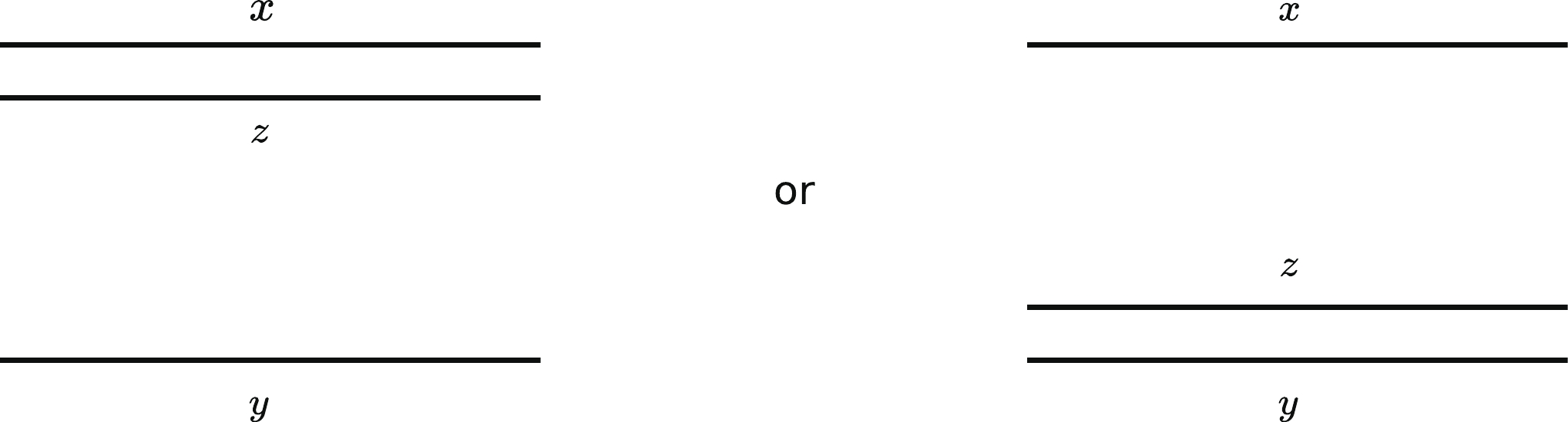
Figure 1. Transverse coordinates of the parent and daughter dipoles in the saturation region.
$ K^{{\rm{LO}}}(r, r_1, r_2) \simeq \frac{\bar{\alpha}_s}{2 \pi} \frac{1}{r_1^2}, $

(7) and Eq. (6) can be rewritten as
$ \frac{\partial}{\partial Y} S(r, Y) \simeq -2\frac{\bar{\alpha}_s}{2\pi}\pi\int_{1/Q_s^2}^{r^2}{\rm d}r_1^2 \frac{1}{r_1^2} S(r, Y), $

(8) where the factor
$ 2 $ on the r.h.s comes from the symmetry of the aforementioned two integral regions. By performing integrals over the variables$ r_1 $ and Y in Eq. (8), the analytic solution of the LO BK equation in the saturation region can be obtained as [35, 36],$\begin{aligned}[b] S(r, Y) =& \exp\left[-\frac{c \bar{\alpha}_s^2}{2}(Y-Y_0)^2\right]S(r, Y_0)\\ =& \exp\left[-\frac{\ln^2(r^2Q_s^2)}{2c}\right]S(r, Y_0), \end{aligned}$

(9) where c is a constant from the saturation momentum
$ Q_s^2(Y) = \exp\left[c\bar{\alpha}_s(Y-Y_0)\right]Q_s^2(Y_0) $ with$ Q_s^2(Y_0)r^2 = 1 $ . The solution in Eq. (9) was first derived in Ref. [35], which is called as the Levin-Tuchin formula. It can be seen that the exponent of the scattering matrix S has a quadratic rapidity dependence, which leads to the scattering matrix being extremely small when the rapidity is large. In terms of the relation between the scattering matrix S and scattering amplitude T,$ T = 1 - S $ , it is known that the evolution speed of the scattering amplitude is too high, which renders the LO BK equation to insufficiently describe the experimental data from HERA [8, 9]. Therefore, the NLO corrections to the LO BK equation should be taken into account, such as the running coupling effect, which can introduce modifications to the evolution kernel, thus reducing the evolution speed of the dipole amplitude. -
The strong coupling constant
$ \alpha_s $ in the LO BK Eq. (3) was assumed to be constant when the LO BK equation was derived, which makes the LO BK equation a leading logarithm (LL) accuracy evolution equation. A naive way to promote it to include the NLO correction is to replace$ \alpha_s\rightarrow\alpha_s(r^2) $ in the LO BK equation [37]$ K^{\rm{PDRCP}}(r,r_1,r_2) = \frac{\alpha_s(r^2)N_c}{2 \pi^2} \frac{r^2}{r_1^2r_2^2}, $

(10) where the argument of the coupling constant is the transverse size of the parent dipole. For
$ \alpha_s $ , we shall use the running coupling at one loop accuracy$ \alpha_s(r^2) = \frac{1}{b\ln\left(\dfrac{1}{r^2\Lambda^2}\right)}, $

(11) with
$ b = (11N_c-2N_f)/12\pi $ .Another running coupling prescription has been proposed recently in Refs. [33, 34, 38, 39], where it was found that using the size of the smallest dipole as the argument of the coupling constant is favored by the HERA data at a phenomenological level, which is referred to as the SDRCP. In the case of the SDRCP, the kernel can be written as
$ K^{\rm{SDRCP}}(r,r_1,r_2) = \frac{\alpha_s(r_{{\rm{min}}}^2)N_c}{2 \pi^2} \frac{r^2}{r_1^2r_2^2} $

(12) with
$ r_{\rm{min}} = {\rm{min}}\{r,r_1,r_2\}.$ We would like to point out that all the following studies employing running coupling in this paper use the SDRCP unless otherwise specified.
Eq. (10) presents a naive way to include the running coupling effect into the LO BK equation, which is insufficient. The real running coupling corrections to the LO BK equation were calculated by including the contributions from the quark bubbles in the gluon lines. The calculations have been performed with two prescriptions by Balitsky in Ref. [14] and Kovchegov and Weigert in Ref. [15]. We will not present the details of the derivations of the rcBK equation and will simply quote the results here as such details are beyond the scope of this paper.
The rcBK equation is given by
$ \frac{\partial}{\partial Y} S(r, Y) = \int{\rm d}^2 r_1 \,K^{{\rm{rc}}}(r, r_1, r_2) \left[S(r_1, Y)\,S(r_2, Y)-S(r, Y)\right], $

(13) where
$ K^{{\rm{rc}}}(r, r_1, r_2) $ is the running coupling evolution kernel. It can be observed that the rcBK equation Eq. (13) has the same structure as the LO BK equation Eq. (3) but for the evolution kernel modified by the running coupling effect. There are two different (Balitsky and Kovchegov-Weigert) prescriptions for the kernel of the rcBK equation as mentioned above. In the case of the Balitsky prescription [14], the running coupling kernel can be written as$\begin{aligned}[b] K^{{\rm{rcBal}}}(r, r_1, r_2) =& \frac{N_c\alpha_s(r^2)}{2\pi^2}\left[\frac{r^2}{r_1^2r_2^2} + \frac{1}{r_1^2}\left(\frac{\alpha_s(r_1^2)}{\alpha_s(r_2^2)}-1\right) \right.\\&\left.+ \frac{1}{r_2^2}\left(\frac{\alpha_s(r_2^2)}{\alpha_s(r_1^2)}-1\right)\right]. \end{aligned}$

(14) Under the Kovchegov-Weigert prescription [15], the running coupling kernel is given by
$\begin{aligned}[b] K^{{\rm{rcKW}}}(r, r_1, r_2) =& \frac{N_c}{2\pi^2}\left[ \alpha_s(r_1^2)\frac{1}{r_1^2}- 2\,\frac{\alpha_s(r_1^2)\,\alpha_s(r_2^2)}{\alpha_s(R^2)}\,\right.\\&\times\left.\frac{ { r}_1\cdot { r}_2}{r_1^2\,r_2^2}+ \alpha_s(r_2^2)\frac{1}{r_2^2} \right],\end{aligned} $

(15) with
$ R^2(r, r_1, r_2) = r_1\,r_2\left(\frac{r_2}{r_1}\right)^ {\textstyle\frac{r_1^2+r_2^2}{r_1^2-r_2^2}-2\,\frac{r_1^2\,r_2^2}{ { r}_1\cdot{ r}_2}\frac{1}{r_1^2-r_2^2}}. $

(16) It should be noted that we found an interesting result in our previous studies in Ref. [40], where the Balitsky and Kovchegov-Weigert kernels reduce to the same one under the saturation condition
$ K^{{\rm{rc}}}(r, r_1, r_2) = \frac{N_c}{2\pi^2}\frac{\alpha_s(r_1^2)}{r_1^2}, $

(17) which indicates that the running coupling kernel is independent of the choice of prescription in the saturation region.
To analytically solve the rcBK equation in the saturation region, we substitute the simplified kernel Eq. (17) into Eq. (13) to obtain
$\begin{aligned}[b] \frac{\partial}{\partial Y} S(r, Y) =& \frac{N_c}{2\pi^2} \int\,{\rm d}^2 r_1 \frac{\alpha_s(r_1^2)}{r_1^2} \\&\times\left[S(r_1, Y)\,S(r_2, Y)-S(r, Y)\right]. \end{aligned}$

(18) Under the saturation condition, as it is known that the scattering matrix is small, the quadratic term of the S-matrix in Eq. (18) can therefore be neglected. Eq. (18) reduces to
$ \frac{\partial S(r,Y)}{\partial Y}\simeq- 2\int_{1/Q_s}^{r}\,{\rm d}^2 r_1 \,\frac{\bar{\alpha}_s(r_1^2)}{2\pi r_1^2}S(r, Y), $

(19) where the upper and lower bounds are determined in the same way as the LO BK equation in section IIA, and the factor
$ 2 $ on the r.h.s of Eq. (19) results from the symmetry of the two integral regions, as shown in Fig. 1. By computing the integral over the variables$ r_1 $ and Y in Eq. (19), the analytic solution of the rcBK equation can be obtained [40]:$ \begin{aligned}[b]S(r,Y) =& \exp\left\{-\frac{N_c}{b\pi}(Y-Y_0)\left[\ln\left(\frac{\sqrt{c(Y-Y_0)}}{\ln\dfrac{1}{r^2\Lambda^2}}\right)-\frac{1}{2}\right]\right\}S(r, Y_0) \\ =& \exp\left\{-\frac{N_c}{bc_0\pi}\ln^2\frac{Q_s^2}{\Lambda^2}\left[\ln\left(\frac{\ln\dfrac{Q_s^2}{\Lambda^2}}{\ln\dfrac{1}{r^2\Lambda^2}}\right)-\frac{1}{2}\right]\right\}S(r, Y_0), \end{aligned} $

(20) where
$ Q_s $ is the saturation momentum in the running coupling case [41],$ \ln\frac{Q_s^2}{\Lambda^2} = \sqrt{c_0(Y-Y_0)} + {\cal{O}}(Y^{1/6}), $

(21) where
$ c_0 $ is a constant. In Eq. (20), it can be seen that the exponent of the S-matrix has a linear rapidity dependence in the running coupling case, while the exponent of the S-matrix quadratically depends on the rapidity in the fixed coupling case, as defined in Eq. (9). The change in the rapidity of the S-matrix from quadratic to linear dependence implies that the evolution of the dipole amplitude is slowed down by the running coupling effect, which is in agreement with the theoretical expectations [14, 29]. In addition, phenomenological studies of the HERA experimental data in Refs. [8, 9] showed that the rcBK equation produces a significant improvement in the description of the HERA data, which indicates the importance of the NLO corrections. -
It is known that the rcBK equation only includes the contributions from the quark bubbles, while a full NLO evolution equation should consider contributions from the quark and gluon bubbles, along with those from the tree gluon diagrams with quadratic and cubic nonlinearities. The authors in Ref. [16] presented a comprehensive derivation and obtained a full NLO BK equation that includes all the above-mentioned NLO corrections. However, it has been found that the full NLO BK equation is unstable, as the dipole amplitude resulting from the full NLO BK equation can decrease with increasing rapidity and can even become a negative value [22]. The reason for this instability can be traced to a large contribution from a double-logarithm in the kernel of the full NLO BK equation [22]. To solve the unstable problem, a novel method was devised in Ref. [21] to resum the double transverse logarithms to all orders, and the authors obtained a resummed BK equation that governs the evolution in the double logarithmic approximation (DLA). Soon after the development of the DLA BK equation, it was found that the single transverse logarithms (STL) also have large corrections to the BK equation. By combining the single and double logarithmic corrections, a collinearly improved (ci) BK equation was obtained, which is given by [38]
$\begin{aligned}[b] \frac{\partial S(r, Y)}{\partial Y} =& \int {\rm d}^2r_1K^{{\rm{ci}}}(r,r_1,r_2)[S(r_1, Y)S(r_2, Y)\\&- S(r, Y)], \end{aligned}$

(22) where the collinearly improved evolution kernel is [23]
$ K^{{\rm{ci}}}(r,r_1,r_2) = \frac{\bar{\alpha}_s}{2\pi}\frac{r^2}{r_1^2r_2^2}K^{{\rm{STL}}}K^{{\rm{DLA}}} ,$

(23) with
$ K^{{\rm{STL}}} = \exp\bigg\{- \bar{\alpha}_s A_1\bigg|\ln\frac{r^2}{{\rm{min}}\{r_1^2, r_2^2\}}\bigg|\bigg\} ,$

(24) and
$ K^{{\rm{DLA}}} = \frac{J_1\bigg(2\sqrt{ \bar{\alpha}_s \rho^2}\bigg)}{\sqrt{ \bar{\alpha}_s\rho^2}}. $

(25) The constant
$ A_1 = 11/12 $ in Eq. (24) is the DGLAP anomalous dimension, and$ J_1 $ in Eq. (25) is the Bessel function of the first kind with$ \rho = \sqrt{\ln \Bigg(\frac{r_1^2}{r^2}\Bigg)\ln \Bigg(\frac{r_2^2}{r^2}\Bigg)}. $

(26) We would like to point out that when
$ \ln (r_1^2/r^2) \ln (r_2^2/r^2) $ $< 0 $ , an absolute value is used, and the Bessel function of the first kind$ J_1 $ changes to the modified Bessel function of the first kind$ I_1 $ [38].To analytically solve Eq. (22) in the saturation region, the saturation condition should be applied, which implies that the scattering matrix is very small. Thus, one can neglect the quadratic term in Eq. (22) and only retain the linear term; then, Eq. (22) becomes
$ \frac{\partial S(r, Y)}{\partial Y} \simeq - 2\int_{1/Q_s}^{r} {\rm d}^2r_1\frac{\bar{\alpha}_s}{2\pi}K^{{\rm{CI}}}S(r, Y), $

(27) where the upper and lower bounds of the integral are determined in the same way as that in section IIA. As in the previous subsections, we work in the regime
$ 1/Q_s\ll |{{r}}_1|\ll |{{r}}|,\; |{{r}}_2|\sim|{{r}}| $ . Therefore, we have$ \ln(r^2_2/r^2)\simeq0 $ leading to$ \rho = 0 $ , which implies that the DLA kernel$ K^{{\rm{DLA}}}\simeq 1 $ . This outcome confirms the statement that the double logarithm only plays a significant role in the weak scattering phase-space [21]. Under the approximation mentioned above,$ \frac{\partial S(r, Y)}{\partial Y} \simeq -2\int^{r}_{1/Q_s} {\rm d}^2r_1\frac{\bar{\alpha}_s}{2\pi}\frac{r^2}{r_1^2r_2^2}\Bigg[\frac{r^2}{{\rm{min}}(r_1^2,r_2^2)}\Bigg]^{\pm\bar{\alpha}_sA_1}S(r, Y), $

(28) whose solution is
$ \begin{aligned}[b] S(r, Y) =& \exp\Bigg\{-\frac{N_c}{2b^2\pi}(Y-Y_0)\Bigg[\frac{3N_cA_1-b\pi}{\pi}+\frac{b\pi-N_cA_1}{\pi}\\&\left.\times\ln\left(\frac{c_0(Y-Y_0)}{\ln^2\dfrac{1}{r^2\Lambda^2}}\right)\right] -\frac{2N_c^2A_1}{b^2\pi^2c_0}\sqrt{c_0(Y-Y_0)}\ln r^2\Lambda^2\Bigg\}\\S(r, Y_0) =&\exp\Bigg\{-\frac{N_c}{2b^2\pi c_0}\ln^2\frac{Q_s^2}{\Lambda^2}\Bigg[\frac{3N_cA_1-b\pi}{\pi}\\&\left.+\frac{b\pi-N_cA_1}{\pi}\ln\left(\frac{\ln^2\dfrac{Q_s^2}{\Lambda^2}}{\ln^2\dfrac{1}{r^2\Lambda^2}}\right)\right] \\ &-\frac{2N_c^2A_1}{b^2\pi^2c_0}\ln\frac{Q_s^2}{\Lambda^2}\ln r^2\Lambda^2\Bigg\}S(r, Y_0). \end{aligned} $

(29) It should be noted that the dominant terms in the exponents of Eqs. (20) and (29) have linear rapidity dependence once the SDRCP is applied, which is a law defined in Ref. [34]. This outcome implies that the running coupling correction has a dominant effect over all the aforementioned NLO corrections, such as the resummations of double and single transverse logarithms, in the suppression of dipole evolution.
-
In the previous section, all the BK equations were derived by following the evolution in terms of the rapidity of the projectile (Y). However, recent studies in Ref. [26] have found that the NLO BK equation in Y must be re-established according to the rapidity of the dense target (
$ \eta $ ), as the evolution of the rapidity Y could cause instability to the NLO BK equation. In this section, we shall discuss the non-local ciBK equation in$ \eta $ and its extended version, which includes sub-leading double logarithms from the region beyond the strong time-ordering [27]. The evolution equations in the$ \eta $ -representation shall be solved analytically in the fixed and running coupling cases in the saturation region. The results are compared to the solutions obtained in the Y-representation. -
The non-local ciBK equation was reformulated via change of variables
$ \eta\equiv Y-\rho $ to transform the BK equation from the Y-representation to the$ \eta $ -representation,$ \bar{S}(r,\eta) \equiv S(r, Y = \eta+\rho), $

(30) where
$ \rho = \ln1/(r^2Q_0^2) $ . The non-local ciBK equation can be written as [26]$ \begin{aligned}[b] \frac{\partial \bar{S}(r,\eta)}{\partial\eta} =& \int {\rm d}^2r_1\frac{\bar{\alpha}_s}{2\pi}\frac{r^2}{r_1^2r_2^2}\Theta(\eta-\delta_{r,r_1,r_2})\big[\bar{S}(r_1,\eta-\delta_{r_1,r})\bar{S}(r_2,\eta-\delta_{r_2,r})-\bar{S}(r,\eta)\big] \\ & -\int {\rm d}^2r_1\frac{\bar{\alpha}_s^2}{4\pi}\frac{r^2}{r_1^2r_2^2}\ln\frac{r_2^2}{r^2}\ln\frac{r_1^2}{r^2}\big[\bar{S}(r_1,\eta)\bar{S}(r_2,\eta)-\bar{S}(r,\eta)\big] \\ &+\int {\rm d}^2r_1{\rm d}^2r'_1\frac{\bar{\alpha}_s^2}{2\pi^2}\frac{r^2}{r'^2{r'_1}^2r_2^2}\Big[\ln\frac{{r'_2}^2}{r^2}+\delta_{r'_2,r}\Big]\bar{S}(r'_1,\eta)\big[\bar{S}(r',\eta)\bar{S}(r_2,\eta)-\bar{S}(r'_2,\eta)\big] +\bar{\alpha}_s^2\times ''{\rm{regular}}'', \end{aligned} $

(31) where the rapidity shifts
$ \delta_{r,r_1,r_2} $ and$ \delta_{r_1,r} $ are defined as$ \delta_{r,r_1,r_2} = {\rm{max}}\Bigg\{0,\ln\frac{r^2}{{\rm{min}}\{r_1^2,r_2^2\}}\Bigg\}, $

(32) and
$ \delta_{r_1,r} = {\rm{max}}\Bigg\{0,\ln\frac{r^2}{r_1^2}\Bigg\}, $

(33) and similar expressions are defined for
$ \delta_{r_2,r} $ . It should be noted that on the r.h.s of Eq. (31), there are only two NLO terms displayed explicitly. All other NLO terms are collectively denoted as "regular." The roles of the rapidity shift$ \delta_{r,r_1,r_2} $ and the step function in Eq. (31) are to introduce constraints on the soft-to-hard evolution [26]. We would like to point out that if the sub-leading double logarithm corrections located beyond the strong-ordering region are taken into account, the kernel in Eq. (31) shall be modified by the Sudakov factor, leading to an improved evolution equation called the non-local SSBK equation [27].Next, we will solve the non-local ciBK equation analytically in the saturation region. As known from the previous integrals in Eqs. (6) and (19), the integral in Eq. (31) is governed either by the region
$ 1/\bar{Q}_s\ll $ $ |{{{r}}_{\bf{1}}}|\ll |{{r}}| $ and$ |{{{r}}_{\bf{2}}}|\sim |{{r}}| $ or$ 1/\bar{Q}_s\ll |{{{r}}_{\bf{2}}}|\ll |{{r}}| $ and$ |{{{r}}_{\bf{1}}}|\sim |{{r}}| $ , where$ \bar{Q}_s $ plays the role of the saturation scale$ \bar{Q}_s^2(\eta) = \exp\big[\bar{c}\bar{\alpha}_s(\eta-\eta_0)\big]\bar{Q}_s^2(\eta_0). $

(34) We choose to work in the former region, where the S-matrix is negligibly small, and can thus neglect the quadratic term in Eq. (31). In addition,
$ \ln(r_2^2/r^2)\sim0 $ leads to the second term on the r.h.s of Eq. (31) to be negligible. The non-local ciBK equation reduces to$ \frac{\partial \bar{S}(r,\eta)}{\partial\eta} \simeq -2\int_{1/\bar{Q}_s}^{r} {\rm d}^2r_1\frac{\bar{\alpha}_s}{2\pi}\frac{1}{r_1^2}\Theta(\eta-\delta_{r,r_1,r_2})\bar{S}(r,\eta). $

(35) -
In the fixed coupling case, it is known that the QCD coupling can be viewed as a constant. Thus,
$ \bar{\alpha}_s $ in Eq. (35) can be factorized out of the integral,$ \frac{\partial \bar{S}(r,\eta)}{\partial\eta} \simeq -\frac{\bar{\alpha}_s}{\pi}\int_{1/\bar{Q}_s}^{r} {\rm d}^2r_1\frac{1}{r_1^2}\bar{S}(r,\eta), $

(36) whose solution is [26]
$\begin{aligned}[b] \bar{S}(r,\eta) =& \exp\bigg[-\frac{\bar{c} \bar{\alpha}_s^2}{2}(\eta-\eta_0)^2\bigg]\bar{S}(r,\eta_0)\\= &\exp\bigg[-\frac{\ln^2(r^2\bar{Q}_s^2)}{2\bar{c}}\bigg]\bar{S}(r,\eta_0). \end{aligned}$

(37) Comparing Eq. (37) with Eq. (9), it can be easily observed that both have quadratic rapidity dependence except for different coefficients in the exponent, although they are in different rapidity representations. It is known that the value of
$ \bar{c} $ is smaller than c [26], so the S-matrix in the$ \eta $ -representation is larger than that in the Y-representation for the same value of rapidity. -
In the running coupling case, the QCD coupling is a function of the smallest dipole size. The coupling constant in Eq. (35) cannot be factorized out of the integral, and the evolution Eq. (35) becomes
$ \frac{\partial \bar{S}(r,\eta)}{\partial\eta} \simeq -\frac{N_c}{b\pi^2}\int_{1/\bar{Q}_s}^{r} {\rm d}^2r_1\frac{1}{r_1^2\ln\dfrac{1}{r_1^2\Lambda^2}}\bar{S}(r,\eta), $

(38) whose solution is
$ \begin{aligned}[b] \bar{S}(r,\eta) =& \exp\left\{-\frac{N_c}{b\pi}(\eta-\eta_0)\left[\ln\left(\frac{\sqrt{\bar{c}_0(\eta-\eta_0)}}{\ln\dfrac{1}{r^2\Lambda^2}}\right)-\frac{1}{2}\right]\right\}S(r, \eta_0) \\ =& \exp\left\{-\frac{N_c}{b\bar{c}_0\pi}\ln^2\frac{\bar{Q}_s^2}{\Lambda^2}\left[\ln\left(\frac{\ln\dfrac{\bar{Q}_s^2}{\Lambda^2}}{\ln\dfrac{1}{r^2\Lambda^2}}\right)-\frac{1}{2}\right]\right\}S(r, \eta_0), \end{aligned} $

(39) where the running coupling saturation momentum is
$ \ln\frac{\bar{Q}_s^2}{\Lambda^2} = \sqrt{\bar{c}_0(\eta-\eta_0)} + {\cal{O}}(\eta^{1/6}), $

(40) with
$ \bar{c}_0 $ as a constant. It should be noted that Eq. (39) has a rapidity dependence similar to those of Eqs. (20) and (29), except for different coefficients in the exponent, although they are in different rapidity representations. This result indicates that the solution of the non-local ciBK equation also complieswith the law in Ref. [34]. However, we shall see in the next subsection that the solution of the evolution equation including the corrections of the sub-leading double logarithms violates the law mentioned above. -
It has been shown in Ref. [27] that there are significant corrections coming from the regime beyond the strong ordering region, where the sub-leading double logarithms are induced due to the incomplete cancellation between the real corrections and virtual corrections. These double logarithms have typical Sudakov features and can be resummed into an exponential type, resulting in a Sudakov suppressed Balitsky-Kovchegov equation [27]:
$ \frac{\partial S(r, \eta)}{\partial \eta} = \int {\rm d}^2r_1 K^{{\rm{SS}}}(r,r_1,r_2)[S(r_1, \eta)S(r_2, \eta) - S(r, \eta)], $

(41) where the Sudakov suppressed evolution kernel is
$\begin{aligned}[b] K^{{\rm{SS}}}(r,r_1,r_2) =& \frac{\bar{\alpha}_s}{2\pi}\frac{r^2}{r_1^2r_2^2}\frac{1}{2}\Bigg\{\exp\bigg[-\frac{\bar{\alpha}_s}{2}\ln^2\frac{r^2}{r_1^2}\bigg]\\&+\exp\bigg[-\frac{\bar{\alpha}_s}{2}\ln^2\frac{r^2}{r_2^2}\bigg]\Bigg\}. \end{aligned}$

(42) -
In the fixed coupling case, the QCD coupling in Eq. (42) can be set as a constant. Thus, it can be factorized out of the integral when analytically solving Eq. (41) in the saturation region. As in the previous section, we need to use the saturation condition that indicates that the S-matrix is very small, and the non-linear term on the r.h.s of Eq. (41) can be neglected. The SSBK equation becomes a linear evolution equation in S,
$ \frac{\partial S(r, \eta)}{\partial \eta} \simeq -2\frac{\bar{\alpha}_s}{2\pi}\int^{r}_{1/\bar{Q}_s}\!\! {\rm d}^2r_1 \frac{1}{r_1^2}\frac{1}{2}\Bigg\{\exp\bigg[-\frac{\bar{\alpha}_s}{2}\ln^2\frac{r^2}{r_1^2}\bigg] \!+\! 1\Bigg\}S(r, \eta), $

(43) where the upper and lower bounds are determined in the same way as that in the previous section. The factor 2 on the r.h.s of Eq. (43) comes from the symmetry of the two integral regions, as shown in Fig. 1. Performing the integral over
$ r_1 $ and Y in Eq. (43), its solution is obtained as$ \begin{aligned}[b] S(r, \eta) =& \Bigg\{\exp\bigg[-\frac{\sqrt{\pi}}{8\bar{c}}\ln^2r^2\bar{Q}_s^2\bigg] + \exp\bigg[-\frac{1}{4\bar{c}}\ln^2r^2\bar{Q}_s^2\bigg]\Bigg\}\\ S(r, \eta_0) =& \Bigg\{\exp\bigg[-\frac{\sqrt{\pi}\bar{c}}{8}\bar{\alpha}_s^2(\eta-\eta_0)^2\bigg] \\&+ \exp\bigg[-\frac{\bar{c}}{4}\bar{\alpha}_s^2(\eta-\eta_0)^2\bigg]\Bigg\}S(r, \eta_0), \\[-15pt] \end{aligned} $

(44) where we have employed
$ \ln r^2\bar{Q}_s^2 = \bar{c}\bar{\alpha}_s(\eta-\eta_0) $ with$ \bar{c} $ as a constant. Comparing the solution of the SSBK equation in$ \eta $ (44) with that of the LO BK equation in Y (9), it can be clearly seen that the S-matrix in the Sudakov case is larger than the LO one, as the exponential factor in the second term of Eq. (9) on the r.h.s is almost twice as large as that in Eq. (44). In other words, the scattering amplitude T in the Sudakov case becomes smaller than the LO one, which indicates that the evolution of the dipole amplitude is slowed down by the Sudakov effect as compared with the LO one. -
In the running coupling case, the QCD coupling cannot be factorized out of the integral in Eq. (41), as the QCD coupling could be a function of the integral variable. As in the fixed coupling case, Eq. (41) is solved in the saturation region, and therefore, we can neglect the non-linear term and simply keep the linear term in S. Then, Eq. (41) simplifies to
$\begin{aligned}[b] \frac{\partial S(r, \eta)}{\partial \eta} \simeq & -2\int^{r}_{1/\bar{Q}_s} {\rm d}^2r_1 \frac{\bar{\alpha}_s(r^2_{{\rm{min}}})}{2\pi}\frac{1}{r_1^2}\frac{1}{2}\\&\times\Bigg\{\exp\bigg[-\frac{\bar{\alpha}_s}{2}\ln^2\frac{r^2}{r_1^2}\bigg] + 1\Bigg\}S(r, \eta). \end{aligned}$

(45) It should be noted that the kernel in Eq. (45) is simplified based on the fact that the integral is governed by the region either from the transverse coordinate of the emitted gluon approaching the quark leg of the parent dipole,
$ 1/\bar{Q}_s\ll |{{{r}}_{\bf{1}}}|\ll |{{r}}| $ and$ |{{{r}}_{\bf{2}}}|\sim |{{r}}| $ , or the transverse coordinate of the emitted gluon approaching the antiquark leg of the parent dipole,$ 1/\bar{Q}_s\ll |{{{r}}_{\bf{2}}}|\ll |{{r}}| $ and$ |{{{r}}_{\bf{1}}}|\sim |{{r}}| $ ; see Fig. 1. The factor 2 on the r.h.s of Eq. (45) accounts for the symmetry of the integral regions mentioned above. We choose to work in the region$ 1/\bar{Q}_s\ll |{{{r}}_{\bf{1}}}|\ll |{{r}}| $ and$ |{{{r}}_{\bf{2}}}|\sim |{{r}}| $ , and the evolution kernel becomes$ \begin{aligned}[b] K^{{\rm{SS}}}(r,r_1,r_2) = \frac{\bar{\alpha}_s(r^2_{\rm{min}})}{2\pi}\frac{r^2}{r_1^2r_2^2}\frac{1}{2}\Bigg\{\exp\bigg[-\frac{\bar{\alpha}_s}{2}\ln^2\frac{r^2}{r_1^2}\bigg]+\exp\bigg[-\frac{\bar{\alpha}_s}{2}\ln^2\frac{r^2}{r_2^2}\bigg]\Bigg\} \simeq \frac{\bar{\alpha}_s(r^2_{\rm{min}})}{2\pi}\frac{1}{r_1^2}\frac{1}{2}\Bigg\{\exp\bigg[-\frac{\bar{\alpha}_s}{2}\ln^2\frac{r^2}{r_1^2}\bigg] + 1\Bigg\}. \end{aligned} $

(46) Performing the integral over the variables
$ r_1 $ and$ \eta $ in Eq. (45), its solution can be obtained as$ \begin{aligned}[b] S(r, \eta) =& \left\{\exp\left[-\frac{N_c}{4b\bar{c}_0\sqrt{\pi}\ln\dfrac{1}{r^2\Lambda^2}}\left(\frac{2}{3}\ln^3\frac{\bar{Q}_s^2}{\Lambda^2}+\ln\frac{1}{r^2\Lambda^2}\ln^2\frac{\bar{Q}_s^2}{\Lambda^2}\right)\right]\right. \left.+ \exp\left[-\frac{N_c}{b\bar{c}_0\pi}\ln^2\frac{\bar{Q}_s^2}{\Lambda^2}\left(\ln\left(\dfrac{\ln\dfrac{\bar{Q}_s^2}{\Lambda^2}}{\ln\dfrac{1}{r^2\Lambda^2}}\right)-\frac{1}{2}\right)\right]\right\}S(r,\eta_0) \\ =& \left\{\exp\left[-\frac{N_c}{4b\bar{c}_0\sqrt{\pi}\ln\dfrac{1}{r^2\Lambda^2}}\left(\frac{2}{3}\big(\bar{c}_0(\eta-\eta_0)\big)^{\frac{3}{2}}+\ln\frac{1}{r^2\Lambda^2}\bar{c}_0(\eta-\eta_0)\right)\right]\right. + \left.\exp\left[-\frac{N_c}{2b\pi}\bar{c}_0(\eta-\eta_0)\left(\ln\left(\frac{\sqrt{\bar{c}_0(\eta-\eta_0)}}{\ln\dfrac{1}{r^2\Lambda^2}}\right)-\frac{1}{2}\right)\right]\right\}S(r,\eta_0), \end{aligned} $

(47) where the saturation momentum in the running coupling case is used; see Eq. (40). The solution in Eq. (47) deserves several important comments as detailed below:
● Comparing the running coupling solution of the SSBK Eq. (47) with the fixed coupling solution of the SSBK Eq. (44), it can be seen that the rapidity dependence of the dominant term in the exponent changes from the quadratic rapidity dependence Eq. (44) to the rapidity raised to the power of 3/2 dependence Eq. (47), as opposed to the linear dependence. This result does not coincide with the law in Ref. [34], where the solutions of all the NLO evolution equations have linear rapidity dependence once the SDRCP is applied. The reason for this violation comes from the kernel of the SSBK equation modified by the Sudakov factor, which results from the resummation of the sub-leading double logarithm corrections. It should be noted that the sub-leading double logarithms are generated by the incomplete cancellation between the real and virtual corrections in the t-channel calculations [27].
● It can be seen that the solutions of the fixed coupling Eq. (44) and running coupling Eq. (47) SSBK equations have two terms owing to the kernel having two terms; see Eq. (42). The second terms in Eqs. (44) and (47) are similar to the respective ones in the non-local ciBK cases, except for an additional factor
$ 1/2 $ difference in the exponents, which implies that the first terms in Eqs. (44) and (47) potentially come from the incomplete cancellation between the real and virtual corrections.● Interestingly, we find that the dominant term (the first term on the r.h.s of Eq. (47)) of the solution of the SSBK equation with SDRCP
$ \exp(-{\cal{O}}(\eta^{3/2})) $ has a rapidity dependence similar to that obtained by solving the full NLO BK equation in Y with the PDRCP$ \exp(-{\cal{O}}(Y^{3/2})) $ .To conclude, it can be seen that the sub-leading double logarithms resulting from the incomplete cancellation between the real and virtual corrections beyond the strong time-ordering region introduce significant changes to the rapidity dependence of the dipole amplitude not only in the fixed coupling case but also in the running coupling case.
-
In this section, we shall use the numerical method to solve the SSBK equation to test the corresponding analytic solutions obtained in the above section, with focus on the comparison of the numerical results located in the saturation region with the analytic solutions. As it is known that the dipole evolution equations are a set of complicated integro-differential equations, the Runge-Kutta method is needed to solve them on the lattice. The integrals in these equations are performed by adaptive integration routines. In addition, interpolation should be performed during the numerical calculations, as some data points that are not located on the lattice should be estimated. Therefore, the cubic spline interpolation method is employed in this study. To simplify the computation, we employ the translational invariant approximation and assume the S-matrix to be independent of the impact parameter of the collisions,
$ S = S(|r|, Y) $ . In terms of the above discussion, we choose to use the GNU Scientific Library (GSL) to perform the numerical computation, as the GSL includes almost all the functions required by the numerical solution to the evolution equations.To solve the SSBK evolution equations, the McLerran-Venugopalan (MV) model is used as the initial condition [42],
$ S^{{\rm{MV}}}(r, \eta = 0) = \exp\bigg[-\bigg(\frac{r^2\bar{Q}_{s0}^2}{4}\bigg)^{\gamma}\ln\Big(\frac{1}{r^2\Lambda^2}+e\Big)\bigg], $

(48) where we set
$ \bar{Q}^2_{s0} = 0.15\; {\rm{GeV}}^2 $ at$ \eta = 0 $ ,$ \gamma = 1 $ , and$ \Lambda = 0.2\; {\rm{GeV}} $ for simplicity, but$ \bar{Q}^2_{s0} $ and$ \gamma $ shall be free parameters when they are used to fit the HERA data in the next section. The one-loop running coupling with$ N_f = 3 $ and$ N_c = 3 $ , Eq. (11), is used as the QCD coupling in this numerical simulation. To regularize the infrared behavior, the coupling value is fixed at$ \alpha_s(r_{{\rm{fr}}}) = 0.75 $ when$ r>r_{{\rm{fr}}} $ .The left-hand panel of Fig. 2 provides the solutions of the non-local ciBK and SSBK equations as functions of the dipole size in the
$ \eta $ -representation for 4 different rapidities. It should be noted that we have plotted a zoomed in diagram to clearly show the numerical results in the saturation region. It can be seen that the values of the SSBK dipole amplitudes are larger than the non-local ciBK ones for each corresponding rapidity in the saturation region. This outcome is consistent with the analytic findings, Eqs. (39) and (47) in Sec. III, where the linear rapidity dependence in the exponent of the S-matrix in the non-local ciBK case is replaced by the rapidity raised to the power of$ 3/2 $ dependence due to the contribution of the sub-leading double logarithms. The right-hand panel of Fig. 2 shows the solutions of the SSBK equation with the fixed coupling ($ \bar{\alpha}_s = 0.3 $ ) and running coupling constant for 4 different rapidities. The zoomed in diagram is used to clearly illustrate the numerical results in the saturation region. We can see that the respective dipole amplitude with the running coupling constant is smaller than the corresponding one with the fixed coupling constant. This numerical result is in agreement with the analytic results, Eqs. (44) and (47), where the quadratic rapidity dependence in the exponent of the S-matrix is replaced by the linear rapidity dependence once the SDRCP is used. The result also indicates that the running coupling effect plays a significant role in suppressing the evolution of the dipole amplitude in both the Y-representation and$ \eta $ -representation.
Figure 2. (color online) The numerical solutions to the non-local ciBK and SSBK evolution equations in
$ \eta $ -representation for 4 different rapidities. The left-hand panel shows comparisons between the non-local ciBK and SSBK dipole amplitudes with the SDRCP. The right-hand panel shows comparisons between the fixed coupling SSBK and running coupling SSBK dipole amplitudes. The inner diagrams show the zoomed in amplitudes in the saturation region. -
In this section, we describe the HERA data [43] for the inclusive DIS cross-section with the SSBK equation. The actual quantity we shall fit is the reduced
$ \gamma^\ast p $ cross-section, which can be expressed in terms of the transverse,$ \sigma_{{\rm{T}}}^{\gamma^\ast p} $ , and longitudinal,$ \sigma_{{\rm{L}}}^{\gamma^\ast p} $ , cross-sections:$ \sigma_{\rm{red}} = \frac{Q^2}{4\pi^2\alpha_{{\rm{em}}}}\bigg[\sigma_{{\rm{T}}}^{\gamma^\ast p}+\frac{2(1-y)}{1+(1-y)^2}\sigma_{{\rm{L}}}^{\gamma^\ast p}\bigg], $

(49) where
$ y = Q^2/(sx) $ is the inelasticity variable, and s is the squared center of mass collision energy. The transverse and longitudinal cross-sections in Eq. (49) can be written as [7, 33, 38]$ \sigma_{{\rm{T,L}}}^{\gamma^\ast p} = \sum\limits_f\int_0^1{\rm d}z\int {\rm d}^2r|\psi^{(f)}_{\rm{T,L}}(r,z;Q^2)|^2\sigma_{\rm{dip}}^{q\bar{q}}(r,x), $

(50) where
$ |\psi^{(f)}_{\rm{T,L}}|^2 $ is the squared light-cone wave function representing the probability of a virtual photon splitting into a quark-antiquark pair with flavor f and can be written as$\begin{aligned}[b] |\psi^{(f)}_{\rm{T}}(r,z;Q^2)|^2 =& e_q^2\frac{\alpha_{\rm{em}}N_c}{2\pi^2}\big\{\bar{Q}_f^2[z^2+(1-z)^2]\\&\times K^2_1(r\bar{Q}_f)+m_f^2K_0^2(r\bar{Q}_f)\big\}, \end{aligned}$

(51) $ |\psi^{(f)}_{\rm{L}}(r,z;Q^2)|^2 = e_q^2\frac{\alpha_{\rm{em}}N_c}{2\pi^2}4Q^2z^2(1-z)^2K_0^2(r\bar{Q}_f), $

(52) where
$ K_0 $ and$ K_1 $ are the modified Bessel functions of the second kind. The$ \bar{Q}_f $ in Eqs. (51) and (52) is defined as$ \bar{Q}_f^2 = z(1-z)Q^2+m_f^2 $ , where$ m_f $ is the quark mass. It should be noted that we only use three light quarks with$ m_{u,d,s} = 140\; {\rm{MeV}} $ in our fit.The key term in Eq. (50) is the dipole cross-section
$ \sigma_{\rm{dip}} = \sigma_0 \big[1 - S(r, \eta)\big], $

(53) which includes critical information about the scattering between the dipole and target. Here, the S-matrix is calculated by numerically solving the SSBK equation, and
$ \sigma_0 $ is viewed as a free parameter whose value is determined by fitting to the HERA data. We would like to point out that we use the one loop QCD coupling$ \bar{\alpha}_s(r^2) = \frac{1}{b\ln\left(\dfrac{4C^2}{r^2\Lambda^2}\right)} $

(54) to fit the HERA data in terms of the rather successful running coupling scheme in Refs. [8, 9]. We set
$ \Lambda = 0.2 $ GeV and treat$ C^2 $ as a free parameter in our fit. In summary, we have four free parameters,$ \sigma_0 $ ,$ \bar{Q}_{s0}^2 $ ,$ \gamma $ , and$ C^2 $ . The first parameter comes from the dipole cross-section, Eq. (53), the second and third parameters are from the initial condition, Eq. (48), and the final parameter originates from the QCD running coupling, Eq. (54).In the fit, we consider the combined data from HERA for the reduced cross-section in the kinematical range
$ x\leqslant 0.01 $ and$ 0.045\; {\rm{GeV}}^2<Q^2<50\; {\rm{GeV}}^2 $ [43]. The lower limit on$ Q^2 $ is chosen low enough to justify the use of the BK dynamics rather than the DGLAP evolution, and the upper limit is sufficiently large to include a large amount of perturbative data points. Based on the above criteria, we have 252 data points in our fit.With the setup described above, we obtain rather good fits to the HERA data on the reduced cross-section. In Table 1, we present the values of the free parameters. The reasonable value of
$ \chi^2/{{d.o.f}} $ indicates that the SSBK equation with the SDRCP provides a rather successful description of the data. In Fig. 3, we illustrate the reduced cross-section as a function of the Bjorken variable x. It should be noted that, in Fig. 3, we only plot the reduced cross-section for some typical values of$ Q^2 $ , as the others also exhibit the same good quality description. Comparing the data points (solid points in Fig. 3) with the theoretical calculations (triangles in Fig. 3), it can be seen that the values of the reduced cross-section calculated by the SSBK equation are in agreement with the HERA data points. This outcome satisfies the theoretical expectation [26]. Moreover, we also fit the data with the ciBK equation; as shown in Table 1 and Fig. 3, the description from the SSBK equation is slightly better than that from the ciBK equation. To show the rapidity dependence of the saturation momentum, the value of$ Q_s $ is extracted from the fit to the data via the definition$ T(r = 2/ Q_s, \eta) = 1/2 $ . In Fig. 4, we demonstrate the saturation momentum as a function of x. The$ Q_s $ is shown on top of the data points that we use in the fit.dipole amplitude $ \sigma_0 $ /mb

$\bar{Q}_{s0}^2/{\rm{GeV} }^2$ 

$ \gamma $ 

$ \; \; C^2 $ 

$ \chi^{2}/{{d.o.f}} $ 

SSBK 32.513 0.139 1.057 19.445 1.128 ciBK 31.515 0.153 1.052 26.556 1.261 Table 1. Values of the fitting parameters and
$ \chi^{2}/{{d.o.f}} $ from the fit to the reduced cross-section data points from [43].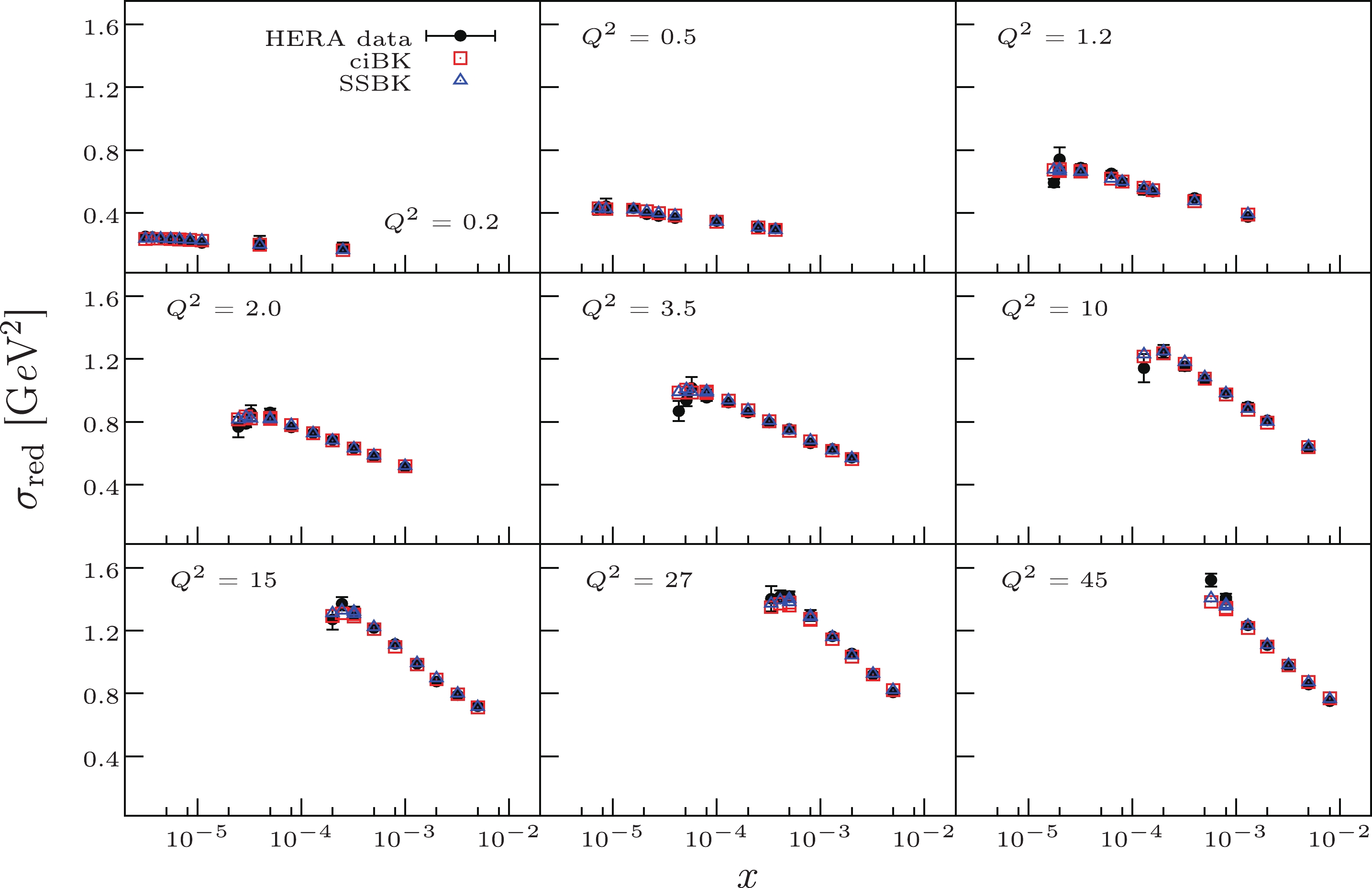
Figure 3. (color online) The reduced cross-section versus x at different values of
$ Q^2 $ . The experimental data points are the combined measurement from the H1 and ZEUS collaborations [43]. We have only plotted the reduced cross-section for some typical values of$ Q^2 $ . The others also show the same good quality. The blue triangles denote the results computed with the SSBK equation. The red squares are the results calculated using the ciBK equation.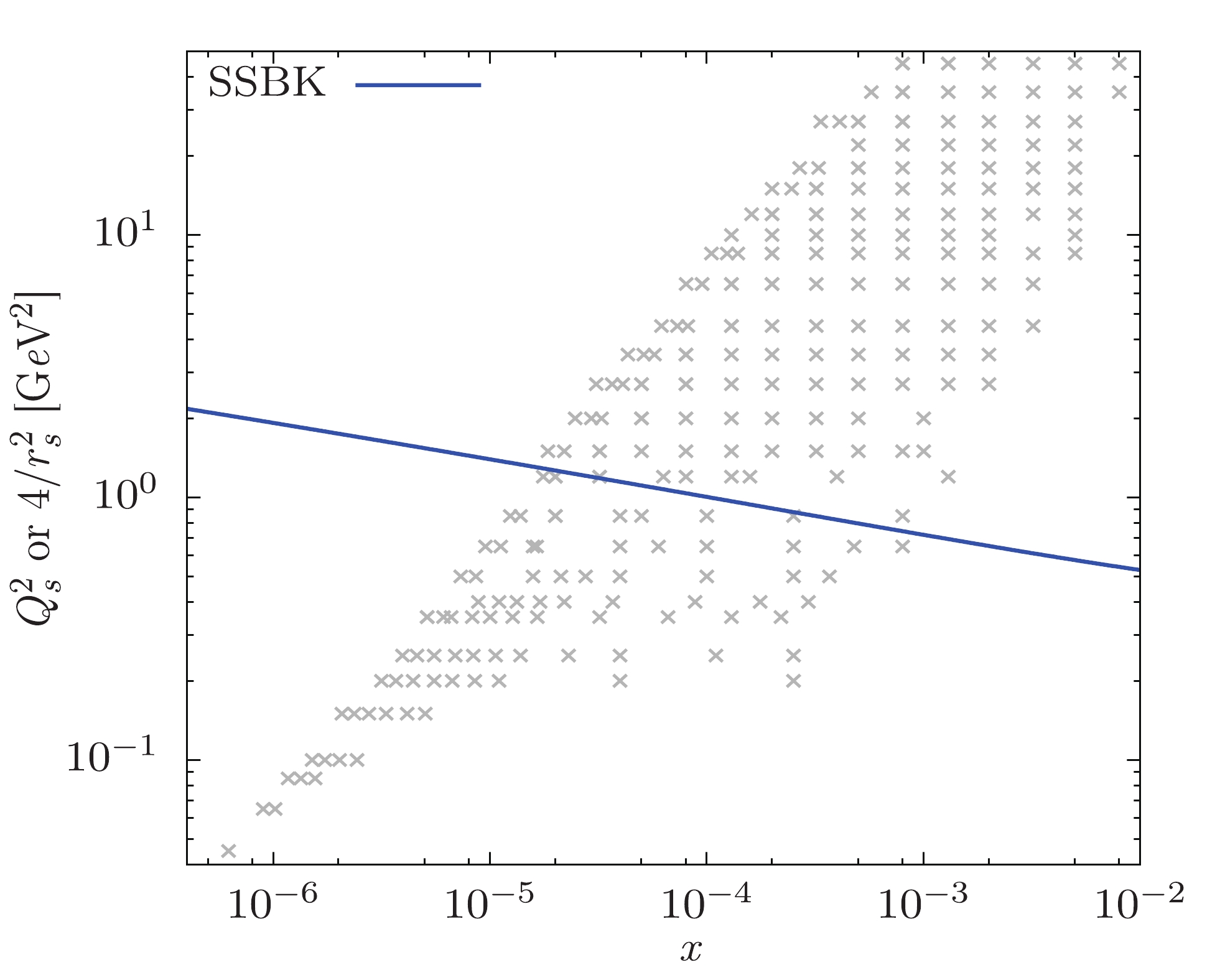
Figure 4. (color online) The squared saturation scale versus x, with
$ Q_s $ defined as$ T(r = 2/Q_s, \eta) = 1/2 $ . -
In this paper, we first presented a review of the analytic solutions of the LO BK, rcBK, and ciBK equations in the Y-representation to provide subsequent comparisons with the SSBK calculations in the
$ \eta $ -representation. This showed that the solution of the LO BK equation has a quadratic rapidity dependence ($ \exp[-{\cal{O}}(Y^2)] $ ) in the exponent of the S-matrix, and the solutions of the rcBK and ciBK equations have linear rapidity dependence ($ \exp[-{\cal{O}}(Y)] $ ) in the exponent of the S-matrix when the SDRCP is used. In the saturation region, we presented, for the first time, the analytic solutions to the SSBK equation whose evolution kernel is modified by the Sudakov factor. The analytic solution of the SSBK equation with the fixed coupling constant shows a rapidity dependence ($ \exp[-{\cal{O}}(\eta^2)] $ ) similar to that of the corresponding solution in the Y-representation. Surprisingly, we found that the analytic solution of the SSBK equation with the SDRCP has$ \exp(-{\cal{O}}(\eta^{3/2})) $ rapidity dependence, as opposed to the law determined in our previous publication, where all the solutions of the NLO evolution equations comply with a linear rapidity dependence in the exponent of the S-matrix when the SDRCP is used. This violation is caused by the Sudakov modified evolution kernel.We numerically solved the SSBK equation to test the analytic findings. From the zoomed in diagram in Fig. 2, it can be seen that the numerical results confirm our analytic outcomes. Finally, we used the numerical solutions of the SSBK equation as the dipole amplitude to fit the HERA data and compared them with the ciBK fitting results. This demonstrates that the SSBK equation may provide a slightly better description of the data than the ciBK equation.
Solution to the Sudakov suppressed Balitsky-Kovchegov equation and its application to HERA data
- Received Date: 2020-08-11
- Available Online: 2021-01-15
Abstract: We analytically solve the Sudakov suppressed Balitsky-Kovchegov evolution equation with fixed and running coupling constants in the saturation region. The analytic solution of the S-matrix shows that the


 DownLoad: