


 Abstract
 HTML
HTML Reference
 Related
 PDF
PDF


-
Quantum chromodynamics (QCD) is considered to be the field theory of hadronic strong interactions. Due to its asymptotic freedom property [1, 2], the QCD strong coupling constant becomes numerically small at short distances, allowing perturbative calculation of high-energy processes. The QCD theory, in the case of a covariant gauge with massless quarks, features three fundamental propagators (corresponding to the gluon, ghost, and quark fields) and four fundamental vertices (i.e., the triple-, four-, ghost-, and quark-gluon vertices). In the literature, various renormalization schemes have been adopted to regularize and remove the ultraviolet divergences that occur at higher perturbative orders. Among these, the momentum space subtraction (MOM) scheme [3-8] has been frequently used alongside the conventional minimum subtraction scheme [9]; it contains a considerable amount of information regarding the various quark and gluon interaction vertices at specific momentums and can enhance convergence in certain cases. Initially, the MOM scheme is defined by renormalizing the three-point vertices of the QCD Lagrangian at the completely symmetric point [3, 4]; i.e., the squared momenta of each external momentum of the vertex are equal. Recently, an asymmetric point at which one of the external momenta vanishes for the three-point vertex has been suggested [7, 10, 11]; this prevents infrared divergence in massless QCD. More explicitly, the minimal MOM (mMOM) scheme [7], which subtracts at the asymmetric point where one external momentum vanishes, has been suggested as an alternative to the original symmetric MOM scheme. It represents an extension of the MOM scheme on the ghost-gluon vertex and allows the strong coupling to be fixed solely by determining the gluon and ghost propagators. There are four further variants of the asymmetric MOM scheme: one with a vanishing momentum for the incoming ghost in the ghost-gluon vertex, one with a vanishing momentum for the incoming quark in the quark-gluon vertex, and two that tackle the case of a vanishing momentum for the incoming gluon in the triple-gluon vertex. Following Ref. [11], we label these MOM schemes as MOMh, MOMq, MOMg, and MOMgg [12, 13], respectively. MOM schemes have been successfully applied in various high-energy processes; however, in contrast to the minimum subtraction scheme, the MOM scheme has been found to violate gauge invariance. It is interesting to show whether the gauge dependence exists for all (typical) MOM schemes and to find a MOM scheme with minimum gauge dependence.
The strong coupling is the most important component of pQCD; its exact magnitude at any scale must be known when deriving an accurate pQCD prediction. The scale running behavior of the strong coupling is controlled by the renormalization group equation (RGE) or the
$ \beta $ -function. The RGE of the MOM scheme can be related to that of the modified minimal subtraction scheme (i.e., the$ \overline{\rm{MS}} $ scheme [14]) via the proper relations. At present, explicit expressions for the$ \{\beta_i\} $ -functions under the$ \overline{\rm MS} $ scheme have been found up to the five-loop level (see Refs. [15-25]). Thus, the five-loop$ \{\beta_i\} $ -functions for the MOM schemes (i.e., mMOM, MOMh, MOMq, MOMg, and MOMgg) can be determined using the known five-loop relations [7, 11, 26, 27] of the$ \overline{\rm{MS}} $ scheme. Another method of deriving the running behavior of the MOM scheme's strong coupling (up to the five-loop level) can be found in Ref. [28]. A key component for solving the$ \beta $ -function is the QCD asymptotic scale$ \Lambda $ . The asymptotic scale in the$ \overline{\rm MS} $ -scheme can be fixed by using the PDG world average of the strong coupling constant at the scale of the$ Z^0 $ boson mass$ \alpha^{\overline{\rm MS}}_s(M_Z) = $ $0.1181\pm 0.0011 $ ; this results in$ \Lambda^{n_f = 5}_{\overline{\rm MS}} = 0.210\pm0.014 $ GeV [29]. The asymptotic scale for the MOM scheme can be derived using the Celmaster–Gonsalves relation [3-7]:$ \frac{\Lambda_{\rm{MOM}}}{\Lambda_{\overline{\rm{MS}}}} = \exp \left[\frac{-b_{1}(\xi^{\rm MOM})}{2 \beta_0}\right]. $

(1) Here,
$ \xi^{\rm MOM} $ is the gauge parameter, and$ b_{1}(\xi^{\rm MOM}) $ is the next-to-leading order (NLO) coefficient of the perturbative series of$ \alpha_{s}^{\rm{MOM}} $ expanded over$ \alpha_{s}^{\overline{\rm{MS}}} $ ; i.e.,$\alpha_{s}^{\overline{\rm{MS}}}/4 \pi = \alpha_{s}^{\rm{MOM}}/4 \pi + b_1(\xi) (\alpha_{s}^{\rm{MOM}}/4\pi)^2+ b_2(\xi) (\alpha_{s}^{\rm{MOM}}/4\pi)^3 +\cdots$ . This relation is correct up to all orders [30]. As an example, for the mMOM scheme, we have$ \frac{\Lambda_{\rm{mMOM}}}{\Lambda_{\overline{\rm{MS}}}} = \exp \left[\frac{\left(9 \xi^{2, \rm mMOM}+18 \xi^{\rm mMOM} +169\right)C_A-80 T n_f}{264 C_A-96 T n_f}\right], $

(2) where
$ C_A = 3 $ and$ T = 1/2 $ for the SU(3) color group, and$ n_f $ is the active flavor number.The MOM scheme could be a useful alternative to the
$ \overline{\rm{MS}} $ scheme for studying the behavior and truncation uncertainty of the perturbation series. Many MOM applications have been considered in the literature; e.g., two typical MOM applications for the Higgs boson's decay to gluons and the R-ratio for electron-positron annihilation can be found in Refs. [6, 30-33]. Moreover, the processes involving three- and four-gluon vertices provide an important platform for studying the renormalization scale-setting problem. For the three-gluon vertex, it has already been found that the typical momentum flow appearing in the three-gluon vertex should be a function of the virtuality of three external gluons [34]. For example, because of the improved convergence, a more accurate and reliable pQCD prediction for the Pomeron intercept can be achieved under the MOM scheme than under the$ \overline{\rm{MS}} $ scheme [35-38]. The MOM scheme can also help to avoid the small-scale problem that occurs under the$ \overline{\rm{MS}} $ scheme [39, 40]①.The Higgs boson is a crucially important component of the Standard Model (SM), and its various decay channels are important components of Higgs phenomenology. Of these decay channels, the decay width of
$ H\to g g $ has been calculated up to the five-loop level under the$ \overline{\rm{MS}} $ scheme [41-50]. Using the relations among the strong coupling constants under various renormalization schemes, one can obtain the five-loop MOM expression for the Higgs boson decay width$ \Gamma(H\to gg) $ from the known$ \overline{\rm{MS}} $ expression. A method of transforming the pQCD predictions from one renormalization scheme to another has been presented in detail in Ref. [51]. In this paper, we adopt the decay width$ \Gamma(H\to gg) $ up to the five-loop QCD contribution as an explicit example, to demonstrate how the gauge dependence of the MOM prediction behaves with increasing perturbative orders.Following standard renormalization group invariance (RGI), a physical observable (corresponding to an infinite-order pQCD prediction) should be independent of the choice of renormalization scale and scheme. Conventionally, for a fixed-order pQCD prediction, researchers use an estimated renormalization scale together with an arbitrary range to estimate the uncertainty; this leads to the mismatch of the strong coupling constant with its coefficient at each order and subsequently results in conventional renormalization scheme and scale ambiguities. Many scale-setting approaches have been suggested to resolve the renormalization scale ambiguity. Of these, the principle of maximum conformality (PMC) [52-56] has been suggested to eliminate the conventional renormalization scheme and scale ambiguities simultaneously. In contrast to other scale-setting approaches (e.g., the RG-improved effective coupling method [57, 58]; the principle of minimum sensitivity [59-63]; and the sequential BLM procedure [64, 65] and its variant, modified seBLM [66]), the PMC's purpose is not to find an optimal renormalization scale but to fix the running behavior of the strong coupling constant; for this, it uses the RGE, whose argument is referred to as the PMC scale. The PMC scale is physical in the sense that its value reflects the ''correct" typical momentum flow of the process, which is independent of the choice of renormalization scale. After applying the PMC, the convergence of the pQCD series can be greatly improved due owing to the elimination of divergent renormalon terms. The PMC has a solid theoretical foundation; it satisfies standard RGI and all self-consistency conditions of the RGE [67]. Detailed discussions and numerous applications of the PMC can be found in Refs. [68-71]. In this paper, we first adopt the PMC to eliminate the renormalization scale ambiguity; then, we discuss the gauge dependence of the MOM predictions for the decay width
$ \Gamma(H\to gg) $ .The remainder of this paper is organized as follows. In Sec. 2, we explain the basic components and formulas used to transform the strong coupling constants of various MOM schemes into that of the
$ \overline{\rm{MS}} $ scheme; this is important for transforming the known$ \overline{\rm MS} $ pQCD series into a MOM one. In Sec. 3, we briefly review the PMC's single-scale approach, which is adopted to perform our present PMC analysis. In Sec. 4, we discuss the gauge dependence of the decay width$ \Gamma(H\to gg) $ under the five asymmetric MOM schemes mentioned above. Sec. 5 summarizes the paper. Detailed formulas are presented in the Appendices. -
The scale dependence of the strong coupling is controlled by the
$ \beta $ -function expressed as$ \beta(a(\mu)) = \mu^2\frac{\partial a(\mu)}{\partial \mu^2} = -\sum\limits _{i = 0}^{\infty } \beta _i a(\mu)^{i+2}, $

(3) where
$ \mu $ is the renormalization scale,$ a(\mu) \equiv \alpha _s(\mu)/(4 \pi) $ . The$ \{\beta_i\} $ -functions are scheme-dependent, and their expressions up to the five-loop level under the$ \overline{\rm MS} $ -scheme can be found in Refs. [15-25]. For brevity, when there is no possibility of confusion, we set$ a = a(\mu) $ in the following discussions.For an arbitrary renormalization scheme R, the respective renormalizations of the gluon, quark, and ghost fields are of the form
$ (A^B)^b_\nu = \sqrt{Z_3^R} (A^R)^b_\nu , $

(4) $ \psi^B = \sqrt{Z_2^R} \psi^R, $

(5) $ (c^B)^b = \sqrt{\tilde{Z}_3^R} (c^R)^b, $

(6) respectively, where
$ Z_3^R $ ,$ Z_2^R $ , and$ {\tilde{Z}_3^R} $ are the renormalization constants of the gluon field A, quark field$ \psi $ , and ghost field c, respectively. The superscripts "B" and "R" denote the bare and renormalized fields, respectively. The superscript "b" is the color index for the adjoint representation of the gauge group.By using the typical dimensional regularization [72] (we work in
$ D = 4-2\epsilon $ dimensions), the renormalized strong coupling a and gauge parameter$ \xi $ can be written as$ a^B = \mu^{2\epsilon} Z_a^R a^R, $

(7) $ \xi^B = Z_3^R \xi^R, $

(8) where we have used the fact that the gauge parameter is also renormalized by the gluon field renormalization constant. The bare strong coupling is scale invariant, and the D-dimensional
$ \beta $ -function for the renormalized strong coupling can be derived by taking the derivative over both sides of Eq. (7), as follows:$ 0 = \frac{{\rm d}a^{B}}{{\rm d} \ln \mu^{2}} $

(9) $ = \epsilon Z_{a}^{R} a^R \mu^{2 \epsilon}+\frac{{\rm d} Z_{a}^R}{{\rm d} a^R} \frac{{\rm d} a^R}{{\rm d} \ln \mu^{2}} a^R\mu^{2 \epsilon}+Z_{a}^R \frac{{\rm d} a^R}{{\rm d} \ln \mu^{2}} \mu^{2 \epsilon}. $

(10) Then, we obtain
$ \frac{{\rm d} a^R}{{\rm d} \ln \mu^{2}} = -\frac{\epsilon Z_{a}^R a^R}{\dfrac{{\rm d} Z_{a}^R}{{\rm d} a^R} a^R+Z_{a}^R} = -\epsilon a^R+\beta\left(a^R\right). $

(11) The gluon, ghost, and quark self-energies can be renormalized as
$ 1+\Pi_A^R = Z_3^R (1+\Pi_A^B) , $

(12) $ 1+\tilde{\Pi}_c^R = \tilde{Z}_3^R (1 + \tilde{\Pi}_c^B) , $

(13) $ 1+\Sigma_V^R = Z_2^R (1 + \Sigma_V^B), $

(14) and the triple-, ghost-, and quark-gluon vertices can be renormalized as
$ \begin{array}{l} T_i^R = Z_1^R T_i^B, i = 1, 2, \end{array} $

(15) $ \begin{array}{l} {\tilde{\Gamma}}_i^R = {\tilde{Z}}_1^R {\tilde{\Gamma}}_i^B, i = h, g, \end{array} $

(16) $ \begin{array}{l} \Lambda_i^R = \bar{Z}_{1}^R \Lambda_i^B, \Lambda_i^{T,R} = \bar{Z}_1^R \Lambda_i^{T,B}, i = q, g, \end{array} $

(17) where the vertex renormalization constants relate to the field and coupling renormalization constants via the Ward–Slavnov–Taylor identities (i.e., the generalized Ward–Takahashi identities [73-76]) via
$ \sqrt{Z_3^R Z_a^R} = \frac{Z_1^R}{Z_3^R} = \frac{\tilde{Z}_1^R}{\tilde{Z}_3^R} = \frac{\bar{Z}_1^R}{Z_2^R}. $

(18) Under the minimal subtraction scheme (
$ \rm{MS} $ ) [9], in which the ultraviolet divergence ($ {1}/{\epsilon} $ -terms of the pQCD series) is directly subtracted, the renormalized parameters$ Z^{\rm MS}_{k} $ can be written as$ Z^{\rm MS}_{k} = 1+\sum\limits_{n = 1}^{\infty} \left(\sum\limits_{m = 1}^{n} \frac{b^{\rm MS}_{m,n}}{\epsilon^{m}}\right)a^{{\rm MS}, n}, $

(19) where the coefficients
$ b^{\rm MS}_{m,n} $ are free of$ \mu $ -dependence [77]. The renormalized constant$ Z^{\rm MS}_{a} $ is gauge independent and takes the following form:$ \begin{split} Z^{\rm MS}_{a} = & 1-\frac{\beta_{0}}{\epsilon} a^{\rm MS}+\left(\frac{\beta_{0}^{2}}{\epsilon^{2}}-\frac{\beta_{1}}{2 \epsilon}\right) a^{2, {\rm MS}}-\left(\frac{\beta_{0}^{3}}{\epsilon^{3}}-\frac{7 \beta_{0} \beta_{1}}{6\epsilon^{2}}\right. \\& \left.+\frac{\beta_{2}}{3 \epsilon}\right) a^{3, {\rm MS}} +\left(\frac{\beta_{0}^{4}}{\epsilon^{4}}-\frac{23 \beta_{1} \beta_{0}^{2}}{12 \epsilon^{3}}+\frac{20\beta_{2} \beta_{0}+9 \beta_{1}^{2}}{24\epsilon^{2}} \right. \\ & \left.-\frac{\beta_{3}}{4 \epsilon}\right) a^{4, {\rm MS}}-\left(\frac{\beta_{0}^{5}}{\epsilon^{5}} +\frac{172 \beta_{2} \beta_{0}^{2}+157 \beta_{1}^{2} \beta_{0}}{120 \epsilon^{3}} \right.\\ & \left.-\frac{163 \beta_{1} \beta_{0}^{3}}{60 \epsilon^{4}}-\frac{34 \beta_{1} \beta_{2}+39 \beta_{0} \beta_{3}}{60 \epsilon^{2}}-\frac{\beta_{4}}{5 \epsilon}\right)a^{5, {\rm MS}}+\cdots. \end{split} $

(20) Here, the
$ \{\beta_{i}\} $ -functions are for the$ {\rm MS} $ scheme; they are the same for all the other dimensional-like renormalization schemes. This is because the strong couplings among the dimensional-like schemes can be simply related via a scale shift [55]; e.g., the$ \overline{\rm MS} $ scheme differs from the$ {\rm MS} $ scheme by an additional absorbtion of$ \ln 4\pi -\gamma_E $ , which corresponds to redefining the$ {\rm MS} $ scale$ \mu_{\rm MS} $ as$ \mu^2_{\rm MS} = \mu^2_{\overline{\rm MS}}\exp\left(\ln 4\pi -\gamma_E\right) $ . Gross and Wilczek found that the leading-order (LO)$ \{\beta_{i}\} $ -functions under dimensional-like renormalization schemes are gauge independent [78]; more recently, Caswell and Wilczek proved such gauge independence up to all orders [79]②.Using Eq. (8), we obtain the following relations for the strong coupling and gauge parameters between the MOM and
$ \overline{\rm {MS}} $ schemes:$ a^{\rm{MOM}} = \frac{Z_a^{\overline{\rm {MS}}}}{Z_a^{\rm{MOM}}} a^{\overline{\rm {MS}}}, $

(21) $ \xi^{\rm{MOM}} = \frac{Z_3^{\overline{\rm {MS}}}}{Z_3^{\rm{MOM}}}\xi^{\overline{\rm {MS}}}. $

(22) It has been found that the MOM scheme is gauge dependent. Under the MOM scheme [7, 11, 26], the gluon, ghost, and quark self-energies are absorbed into the field renormalization constants at the subtraction point
$ q^2 = -\mu^2 $ , as follows:$ \begin{array}{l} 1+\Pi_A^{\rm{MOM}}(-\mu^2) = Z_3^{\rm{MOM}} \Bigg[1+\Pi_A^B(-\mu^2)\Bigg] = 1 , \end{array} $

(23) $ \begin{array}{l} 1+\tilde{\Pi}_c^{\rm{MOM}}(-\mu^2) = \tilde{Z}_3^{\rm{MOM}}\Bigg[1+\tilde{\Pi}_c^B(-\mu^2)\Bigg] = 1 , \end{array} $

(24) $ \begin{array}{l} 1+\Sigma_V^{\rm{MOM}}(-\mu^2) = Z_2^{\rm{MOM}} \Bigg[1+\Sigma_V^B(-\mu^2) \Bigg] = 1 . \end{array} $

(25) Using Eq. (8), we obtain the following relationship of the gauge parameters between the
$ \overline{\rm{MS}} $ and MOM schemes:$ \begin{array}{l} \xi^{{\rm{MOM}}} = \left(1+\Pi^{{\overline{\rm{MS}}}}_A\right)\xi^{{\overline{\rm{MS}}}}. \end{array} $

(26) In the following subsections, we introduce five asymmetric MOM schemes, explaining the relationships between the strong couplings of those schemes with those in the conventional
$ \overline{\rm MS} $ scheme, as well as their gauge-dependent basic components, which are found by renormalizing the three-point vertices (e.g., the ghost-gluon, gluon-quark, and triple-gluon vertices) at the asymmetric point where one of the external momenta of the vertex vanishes. -
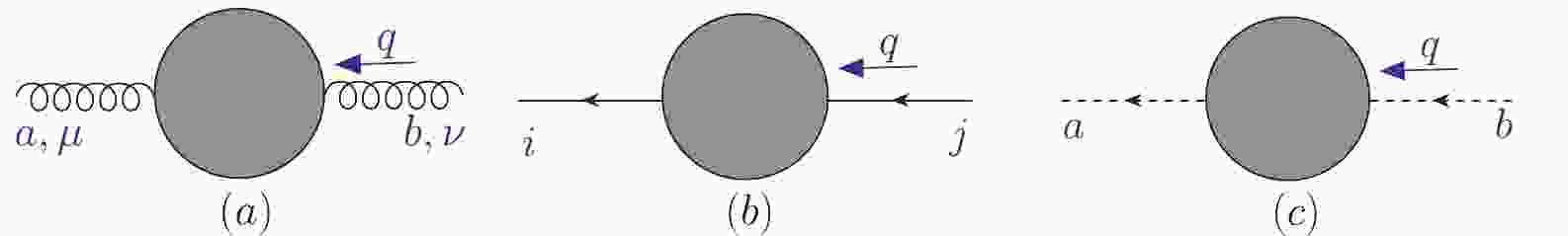
The gluon, quark, and ghost propagators (shown in Fig. 1) are expressed as
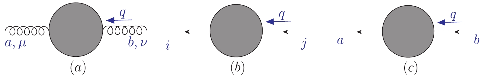
Figure 1. (color online) The gluon, quark, and ghost propagators:
$ \Pi_{\mu \nu}^{a b}(q) $ ,$ \Sigma^{i j}(q) $ , and$ {\tilde{\Pi}}^{a b}(q) $ , respectively.$ D^{ab}_{\mu\nu}(q) = -\frac{\delta^{ab}}{q^2} \biggl[\Bigl( - g_{\mu\nu} + \frac{q_\mu q_\nu}{q^2}\Bigr) \frac{1}{1+\Pi_{A}(q^2)}- \xi \,\frac{q_\mu q_\nu}{q^2}], $

(27) $ S^{ij}(q) = -\frac{\delta^{ij} \not\!\! {q}}{q^2\Bigl(1+\Sigma_V(q^2)\Bigr)}, $

(28) $ \Delta^{ab}(q) = -\frac{\delta^{ab}}{q^2\Bigl(1+\tilde{\Pi}_{c}(q^2)\Bigr)}, $

(29) where a and b are color indices, and i and j denote quark flavors. The gauge parameter
$ \xi = 0 $ corresponds to the Landau gauge,$ \xi = 1 $ corresponds to the Feynman gauge, and so on. The self-energies$ \Pi(q^2) $ ,$ \Sigma_V(q^2) $ , and$ \tilde{\Pi}(q^2) $ can be extracted from the corresponding one-particle irreducible diagrams by applying the proper projection operators [11] (the same holds for the vertex functions discussed below). -
The tree-level ghost-gluon vertex is
$ -{\rm i} g_s f^{abc} q_{\mu} $ , where$ q_{\mu} $ denotes the outgoing ghost momentum. There are two ways of setting one of the external momenta to zero for the ghost-gluon vertex. The first is to set the gluon momentum to zero (as shown in Fig. 2(a)); hence, the renormalized vertex can be written as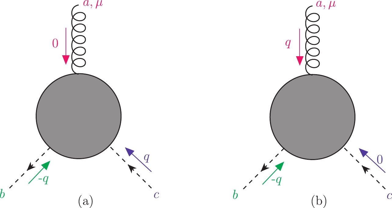
Figure 2. (color online) The ghost-gluon vertex: (a)
$ \tilde{\Gamma}_{\mu}^{a b c}(0; $ -$ q, q) $ for an incoming gluon with zero momentum and (b)$ \tilde{\Gamma}_{\mu}^{a b c}(q; $ -$ q, 0) $ for an incoming ghost with zero momentum.$ \begin{array}{l} \tilde{\Gamma}_{\mu}^{a b c}(0; -q, q) = - {\rm i} g_s f^{abc} q_{\mu} \tilde{\Gamma}_g(q^2), \end{array} $

(30) The second method is to set one of the incoming ghost momenta to zero (as shown in Fig. 2(b)); thus, the renormalized vertex can be written as
$ \begin{array}{l} \tilde{\Gamma}_{\mu}^{a b c}(q; -q, 0) = - {\rm i} g_s f^{abc} q_{\mu} \tilde{\Gamma}_h(q^2). \end{array} $

(31) Here,
$ \tilde{\Gamma}_g(q^2) $ and$ \tilde{\Gamma}_h(q^2) $ denote the Lorentz-invariant function with vanishing gluon or ghost momentum, respectively. At the tree-level, we have$ \begin{array}{l} \tilde{\Gamma}_h(q^2) \bigl|_{\rm{tree}} = \tilde{\Gamma}_g(q^2) \bigl|_{\rm{tree}} = 1. \end{array} $

(32) The MOMh scheme is defined by renormalizing the ghost-gluon vertex (Fig. 2(b)) using the following condition:
$ \begin{array}{l} {\tilde{\Gamma}}_{h}^{\rm{MOMh}}(q^2 = -\mu^2) = {\tilde{Z}}_1^{\rm{MOMh}}{\tilde{\Gamma}}_{h}^B(q^2 = -\mu^2) = 1, \end{array} $

(33) Using Eqs. (15)–(18) and (22)–(25), we can connect the strong coupling in the MOMh scheme to that in the
$ \overline{\rm{MS}} $ scheme through the following equation:$ a^{{\rm{MOMh}}}(\mu) = \frac{\left({\tilde{\Gamma}}_{h}^{{\overline{\rm{MS}}}}(-\mu^2)\right)^{2}a^{{\overline{\rm{MS}}}}(\mu)} {\left(1+\Pi^{{\overline{\rm{MS}}}}_A(-\mu^2) \right)\left(1+\tilde{\Pi}^{{\overline{\rm{MS}}}}_c(-\mu^2)\right)^2}\; . $

(34) In addition, motivated by the non-renormalization of the ghost-gluon vertex in the Landau gauge [76], the vertex renormalization constant for this vertex is chosen to be identical to its value in
$ \overline{\rm{MS}} $ ; that is,$ \begin{array}{l} {\tilde{Z}}_1^{\rm{mMOM}} = {\tilde{Z}}_1^{\overline{\rm{MS}}}, \end{array} $

(35) which is equal to 1 in the Landau gauge. We can then derive the following relation for the coupling constants in those two schemes,
$ a^{{\rm{mMOM}}}(\mu) = \frac{a^{{\overline{\rm{MS}}}}(\mu)}{\left(1+\Pi^{{\overline{\rm{MS}}}}_A(-\mu^2) \right)\left(1+\tilde{\Pi}^{{\overline{\rm{MS}}}}_c(-\mu^2)\right)^2}. $

(36) We present the derivation in Appendix A. It shows that the MOMh scheme is equivalent to the mMOM scheme for the Landau gauge (
$ \xi^{\rm mMOM} = \xi^{\rm MOMh} = 0 $ ). -
There are two non-trivial cases with vanishing incoming external momenta for the quark-gluon vertex: the case of a vanishing incoming gluon momentum (as shown in Fig. 3(a)) and the case of a vanishing quark momentum (as shown in Fig. 3(b)). It is clear that nullifying the incoming quark momentum is equivalent to nullifying the outgoing quark momentum; therefore, the vertex in Fig. 3(a) can be written as
Figure 3. (color online) The quark-gluon vertex: (a)
$ \Lambda_{\mu, i j}^{a}(0; -q, $ $ q) $ with zero incoming gluon momentum and (b)$ \Lambda_{\mu, i j}^{a}(q; -q, $ 0) with vanishing quark momentum.$ \Lambda^a_{\mu,ij}(0; -q, q) = g T^a_{ij} \Bigl[\gamma_\mu \Lambda_g(q^2) + \gamma^\nu \biggl( g_{\mu\nu} - \frac{q_\mu q_\nu}{q^2} )\Lambda_g^T(q^2)\Bigr], $

(37) and the vertex in Fig. 3(b) can be written as
$ \Lambda^a_{\mu,ij}(q; -q, 0) = g T^a_{ij} \Bigl[\gamma_\mu \Lambda_q(q^2) + \gamma^\nu \biggl( g_{\mu\nu} - \frac{q_\mu q_\nu}{q^2} )\Lambda_q^T(q^2)\Bigr]. $

(38) The subscripts "g" in Eq. (37) and "q" in Eq. (38) indicate the functions with vanishing gluon and incoming quark momenta, respectively.
$ T_{ij}^{a} $ is the${ SU(3)}$ color group generator for the quark. At the tree-level, we have$ \begin{array}{l} \Lambda_g(q^2) \bigl|_{\rm{tree}} = \Lambda_q(q^2) \bigl|_{\rm{tree}} \, = \, 1 , \end{array} $

(39) $ \begin{array}{l} \Lambda_g^T(q^2) \bigl|_{\rm{tree}} = \Lambda_q^T(q^2) \bigl|_{\rm{tree}} \, = \, 0 . \end{array} $

(40) The MOMq scheme is defined by renormalizing the quark-gluon vertex with a vanishing incoming quark momentum; for example,
$ \begin{array}{l} \Lambda_{q}^{\rm{MOMq}}(q^2 = -\mu^2) = {\overline{Z}}_{1}^{\rm{MOMq}}(\mu^2)\Lambda_{q}^B(q^2 = -\mu^2) = 1. \end{array} $

(41) Therefore, the relations between the coupling constants in the MOMq and
$ \overline{\rm{MS}} $ schemes is$ a^{{\rm{MOMq}}}(\mu) = \frac{\left(\Lambda_{q}^{{\overline{\rm{MS}}}}(-\mu^2)\right)^{2} a^{{\overline{\rm{MS}}}}(\mu)}{\left(1+\Sigma_V^{{\overline{\rm{MS}}}} (-\mu^2)\right)^{2}\left(1+\Pi^{{\overline{\rm{MS}}}}_{A}(-\mu^2)\right)}. $

(42) -
The triple-gluon vertex is symmetric under the exchange of any two of its gluons. As shown in Fig. 4, we can set the momentum of the right-hand gluon to zero without loss of generality. Under this condition, the triple-gluon vertex generally takes the form
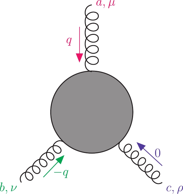
Figure 4. (color online) The triple-gluon vertex with one zero momentum
$ \Gamma_{\mu \nu \rho}^{a b c}(q, -q, 0) $ .$ \begin{split} \Gamma_{\mu \nu \rho}^{a b c}(q, -q, 0) =& - {\rm i} g_s f^{abc} \biggl[(2 g_{\mu\nu} q_\rho - g_{\rho\nu} q_\mu- g_{\mu\rho} q_\nu ) T_1(q^2)\\& -\Bigl( g_{\mu\nu} - \frac{q_\mu q_\nu}{q^2} \Bigr)\, q_\rho T_2(q^2)+q_\mu q_\nu q_\rho T_3(q^2)], \end{split} $

(43) where
$ f^{abc} $ is the structure constant of the${SU(3)}$ color group.$ T_{1}(q^2) $ corresponds to tree-level vertex; i.e.,$ T_1(q^2) \bigl|_{\rm{tree}} = 1 $ .$ T_{2}(q^2) $ is always absent at tree-level but arises from radiative corrections.$ T_{3}(q^2) $ vanishes due to the Ward–Slavnov–Taylor identity for the triple-gluon vertex [11, 26]. The MOMg scheme is defined by renormalizing the aforementioned triple-gluon vertex with a vanishing incoming gluon momentum; for example,$ \begin{array}{l} T_{1}^{\rm{MOMg}}(q^2 = -\mu^2) = Z_{1}^{\rm{MOMg}}(\mu^2) T_{1}^B(q^2 = -\mu^2) = 1. \end{array} $

(44) Therefore, the relation between the coupling constants in the MOMg and
$ \overline{\rm{MS}} $ schemes is$ a^{{\rm{MOMg}}}(\mu) = \frac{\left(T_{1}^{{\overline{\rm{MS}}}}(-\mu^2)\right)^{2}a^{{\overline{\rm{MS}}}}(\mu)} {\left(1+\Pi^{{\overline{\rm{MS}}}}_{A}(-\mu^2)\right)^3}\; . $

(45) The MOMgg scheme is another MOM scheme based on the triple-gluon vertex; it is defined using the following renormalization condition [12, 13]:
$ T_{1}^{\rm{MOMgg}}(q^2 = -\mu^2)-\frac{1}{2}T_{2}^{\rm{MOMgg}}(q^2 = -\mu^2) = 1. $

(46) This gives the following coupling relation between the MOMgg and
$ \overline{\rm{MS}} $ schemes:$ a^{{\rm{MOMgg}}}(\mu) = \frac{\left(T_{1}^{{\overline{\rm{MS}}}}(-\mu^2)-\frac{1}{2}T_{2}^{{\overline{\rm{MS}}}}(-\mu^2)\right)^{2} a^{{\overline{\rm{MS}}}}(\mu)}{\left(1+\Pi^{{\overline{\rm{MS}}}}_{A}(-\mu^2)\right)^3}\; . $

(47) -
The gluon self-energies
$ \Pi^{{\overline{\rm{MS}}}}_A(-\mu^2) $ , the ghost self-energies$ \tilde{\Pi}^{{\overline{\rm{MS}}}}_c(-\mu^2) $ , the quark self-energies$ \Sigma_V^{{\overline{\rm{MS}}}}(-\mu^2) $ , the quark-gluon vertex with vanishing incoming quark momentum$ \Lambda_{q}^{{\overline{\rm{MS}}}}(-\mu^2) $ , the ghost-gluon vertex with vanishing incoming ghost momentum, the two functions$ {\tilde{\Gamma}}_{h}^{{\overline{\rm{MS}}}}(-\mu^2) $ and$ T_1^{{\overline{\rm{MS}}}}(-\mu^2) $ defined in Eq. (45), and the function$ T_2^{{\overline{\rm{MS}}}}(-\mu^2) $ defined in Eq. (47) have all been calculated up to their four-loop QCD corrections under the$ \overline{\rm MS} $ scheme (c.f. Refs. [11, 26]). Using the formulas given in those two references, the relations expressed in Eqs. (34, 36, 42, 45, 47), and Eq. (26), we obtain the expressions for the strong coupling and gauge parameters under various MOM schemes. For convenience, we present these relations in Appendix B.The relations are useful for converting the conventional
$ \overline{\rm MS} $ series into another series under a specific MOM scheme. They are also important for obtaining the MOM scheme$ \beta $ -function, and they thereby determine the correct$ \alpha_s $ -running behavior in the MOM scheme. The MOM$ \beta $ -function is explicitly gauge dependent; it can be written as$ \beta^{\rm{MOM}} = \beta^{\overline{\rm{MS}}}\frac{\partial a^{\rm{MOM}}}{\partial a^{\overline{\rm{MS}}}}+ \frac{\partial \xi^{\overline{\rm{MS}}}}{\partial \ln {\mu^2} }\frac{\partial a^{\rm{MOM}}}{\partial \xi^{\overline{\rm{MS}}}}. $

(48) The anomalous dimension of the gauge parameter
$ \gamma_{\xi}^{\overline{\rm{MS}}} = \frac{1}{\xi^{\overline{\rm{MS}}}} \frac{\partial \xi^{\overline{\rm{MS}}}}{\partial \ln {\mu^2} } $ is equal to$ \left(-\gamma_{A}^{\overline{\rm{MS}}}\right) $ , where$ \gamma_{A}^{\overline{\rm{MS}}} $ is the gluon field's anomalous dimension. Therefore, the MOM-scheme$ \beta $ -function takes the form$ \beta^{\rm{MOM}} = \Bigg(\beta^{\overline{\rm{MS}}}\frac{\partial a^{\rm{MOM}}}{\partial a^{\overline{\rm{MS}}}}-\xi^{\overline{\rm{MS}}}\gamma_{A}^{\overline{\rm{MS}}} \frac{\partial a^{\rm{MOM}}}{\partial \xi^{\overline{\rm{MS}}}}\Bigg)\Bigg |_{\xi^{\overline{\rm{MS}}} \rightarrow \xi^{\rm{MOM}}}^{a^{\overline{\rm{MS}}} \rightarrow a^{\rm{MOM}}}, $

(49) It has been stated that the gauge invariance property of the renormalization scheme is a sufficient but non-necessary property for the factorization of the QCD
$ \beta $ -function [80]. Thus, a reliable$ \alpha_s $ -behavior can be determined and reliable pQCD predictions for various MOM schemes can be made by applying a proper scale-setting approach to deal with the$ \{\beta_i\} $ -terms of the process. -
Conventionally, a pQCD approximant
$ \delta(Q) $ of a physical observable takes the form$ \delta(Q) = a^{p}(\mu)\sum\limits _{i = 1}^{\infty}C_{i}(\mu) a^{i-1}(\mu), $

(50) where Q represents the scale at which the observable is measured, and the index p indicates the
$ \alpha_s $ -order of the leading order (LO) prediction. Here, the perturbative coefficients$ C_i $ are usually in an$ n_f $ power series, where$ n_f $ is the number of light flavors involved in the process. Using the degeneracy relations of different orders [55, 56, 81], the pQCD series can be written as the following$ \beta_i $ series:$ \begin{split} \delta(Q) = & r_{1,0}a(\mu)^p+\Bigg[ r_{2,0} + p \beta_0 r_{2,1} \Bigg]a(\mu)^{p+1} + \Bigg[r_{3,0} + p \beta_1 r_{2,1} + (p+1){\beta _0}r_{3,1} + \frac{p(p+1)}{2} \beta_0^2 r_{3,2} \Bigg]a(\mu)^{p+2} \\ & + \Bigg[ r_{4,0} + p{\beta_2}{r_{2,1}} + (p+1){\beta_1}{r_{3,1}} + \frac{p(3+2p)}{2}{\beta_1}{\beta_0}{r_{3,2}} + (p+2){\beta_0}{r_{4,1}} + \frac{(p+1)(p+2)}{2}\beta_0^2{r_{4,2}} \\ & + \frac{p(p+1)(p+2)}{3!}\beta_0^3{r_{4,3}} \Bigg]a(\mu)^{p+3}+\bigg[r_{5,0}+(p+3) r_{5,1} \beta _0+\frac{(p+2)(p+3)}{2} r_{5,2} \beta _0^2+(p+2) r_{4,1} \beta _1 \\& +\frac{p(p+1)(p+2)(p+3)}{24} r_{5,4} \beta _0^4+\frac{(p+1)(p+2)(p+3)}{6} r_{5,3} \beta _0^3+\frac{(p+1)(2p+5)}{2} r_{4,2} \beta _1 \beta _0 \\ & +\frac{p(3p^2+12p+11)}{6} r_{4,3} \beta _1 \beta _0^2+(p+1) r_{3,1} \beta _2+\frac{p(p+2)}{2} r_{3,2}(2\beta _2 \beta _0+\beta _1^2)+p r_{2,1} \beta _3\bigg]a(\mu)^{p+4}+ \cdots, \end{split} $

(51) where
$ r_{i,0}\; (i = 1,2,3\ldots) $ are conformal coefficients that are generally free from renormalization scale dependence;$ r_{i,j} $ ($ 1\leqslant j<i $ ) are non-conformal coefficients to$ r_{i,j} = \displaystyle\sum_{k = 0}^{j} \left(\begin{array}{l}j\\k\end{array}\right) \ln^{k}(\mu^2/Q^2) \overline{r}_{i-k,j-k} $ , where$ \overline{r}_{m,n} = r_{m,n}|_{\mu = Q} $ . As a subtle point, any$ n_f $ -terms that are irrelevant todetermining the$ \alpha_s $ -running behavior should be kept as a conformal coefficient and cannot be transformed into$ \{\beta_i\} $ -terms [68].For the standard PMC multi-scale approach described in Refs. [53, 55], we must absorb the same type of
$ \{\beta_i\} $ -terms at various orders into the strong coupling constant, in an order-by-order manner. Different types of$ \{\beta_i\} $ -terms (determined from the RGE) result in different running behaviors of the strong coupling constant; hence, they determine the distinct PMC scales at each order. The precision of the PMC scale for high-order terms decreases due to the fewer known$ \{\beta_i\} $ -terms in its higher-order terms. Due to the unknown perturbative terms, the PMC prediction has a residual scale dependence [37]; however, this differs from the arbitrary conventional renormalization scale dependence. The PMC scale, which reflects the correct momentum flow of the process, is independent of the choice of renormalization scale, and its resultant residual scale dependence is generally small, due to the exponential and$ \alpha_s $ suppression [71]. Alternatively, the PMC single-scale approach has been suggested, to suppress the residual scale dependence [82]. In effect, it replaces the individual PMC scales derived under the multi-scale approach with a single scale, using a mean value theorem. The PMC single scale can be regarded as the overall effective momentum flow of the process; it exhibits stability and convergence with increasing order in pQCD, through its use of pQCD approximates. The prediction of the PMC single-scale approach is scheme-independent up to any fixed order [83]; thus, its value satisfies standard RGI. The examples collected in Ref. [83] show that the residual scale dependence arising in the PMC multi-scale approach can indeed be greatly suppressed. In this paper, we adopt the PMC single-scale approach to conduct our discussions.Using the standard procedure for the PMC single-scale approach, we can eliminate all the non-conformal
$ \{\beta_i\} $ -terms and rewrite Eq. (50) as the following conformal series:$ \delta(Q) = \sum\limits_{n \geqslant 1} {r_{n,0}}{a(\overline Q)^{n+p-1}}, $

(52) where the PMC scale
$ \overline Q $ is fixed by requiring that all the non-conformal$ \{\beta_i\} $ -terms vanish. The perturbative series of$ \ln{\overline Q^2}/{Q^2} $ over$ a(Q) $ up to a next-to-next-to-next-to-leading log ($ \rm{N^3LL} $ ) accuracy takes the following form:$ \ln\frac{\overline Q^2}{Q^2} = \lambda_{0} + \lambda_{1}a(Q) + \lambda_{2} a^2(Q)+\lambda_{3} a^3(Q). $

(53) For convenience, we present the perturbative coefficients
$ \lambda_{i} (i = 0,1,2,3) $ in Appendix C. We can observe that neither the resultant PMC conformal series (Eq. (52)) or scale$ \overline{Q} $ contain the renormalization scale ($ \mu $ ); thus, the conventional renormalization scale dependence has been eliminated. A residual dependence for$ \delta(Q) $ remains owing to the unknown terms (e.g., the unknown N$ ^4 $ LL-terms and higher) in the perturbative series (Eq. (53)). -
In this section, we consider the total decay width
$ \Gamma(H\to gg) $ under various MOM schemes as an explicit example, to show how the gauge dependence behaves with increasing numbers of known perturbative orders before and after applying the PMC.Up to the
$ \alpha_s^6 $ -order, the decay width of$ H\to gg $ takes the form$ \Gamma (H\to gg) = \frac{M_H^3 G_F}{36 \sqrt{2} \pi }\sum\limits _{i = 0}^{4} C_{i}(\mu) a^{i+2}(\mu), $

(54) where
$ a(\mu) = \alpha_s(\mu)/(4\pi) $ ,$ \mu $ is the renormalization scale,$ M_H $ is the Higgs boson mass, and$ G_F = 1.16638\times $ $10^{-5}{\rm GeV}^{-2} $ is the Fermi coupling constant. The coefficients$ C_{i\in[0,4]}(M_H) $ of the$ \overline{\rm {MS}} $ scheme can be found in Refs. [41-50]; these coefficients are typically given in an$ n_f $ -power series. Before applying the PMC, the perturbative series (Eq. (54)) should be transformed into the$ \{\beta_i\} $ -series of Eq. (51) with$ p = 2 $ . For convenience, we place the required coefficients$ r_{i,j}(M_H) $ in Appendix D. Then, using the formulas given in Appendix B (which give the perturbative transformations of the strong couplings and gauge parameters for the MOM and$ \overline{\rm MS} $ schemes), we can conveniently transform the perturbative series of$ \Gamma (H\to gg) $ from the$ \overline{\rm {MS}} $ scheme into the MOM scheme. The coefficients at any renormalization scale can be obtained from$ C_{i\in[0,4]}(M_H) $ by using the RGE. Finally, by applying the PMC single-scale setting approach, the pQCD series (Eq. (54)) can be rewritten as the following conformal series$ \Gamma (H\to \ gg) = \frac{M_H^3 G_F}{36 \sqrt{2} \pi } \sum\limits _{i = 1}^{5} r_{i,0} a^{i+1}(\overline Q), $

(55) and the solution of
$ \ln{{\overline Q}^2}/{ M_H^2} $ can be written as a power series in$ a(M_H) $ with an$ \rm{N^3LL} $ -accuracy.To perform the numerical calculation, we adopt the top-quark pole mass
$ m_t = 173.3\; \rm{GeV} $ [84, 85] and the Higgs mass$ M_H = 125.09 \pm 0.21 \pm 0.11 $ $ \rm{GeV} $ [86, 87]; the MOM QCD asymptotic scale is fixed as$ \alpha^{\rm \overline{MS}}_s(M_Z) = 0.1181 $ , along with the Celmaster–Gonsalves relation (Eq. (1)). -
The effective scales
$ \bar{Q} $ (left column) and their corresponding coupling constants$ \alpha_s(\bar{Q}) $ (right column) with respect to the gauge parameter are shown in Fig. 5. At the two-loop level, the determined scale$ \bar{Q} $ is gauge independent; however, at the three-loop level or above, Fig. 5(a1–a5) shows that$ \overline{Q} $ is gauge-dependent under the five aforementioned MOM schemes. This is due to the fact that all the$ r_{i,j} $ terms of MOM schemes are gauge dependent, except for those of the$ i-j = 1 $ terms. For a specific gauge, we observe that the difference between the two nearby values of$ \overline{Q} $ becomes smaller when more loop terms are included; this indicates that the precision of$ \bar{Q} $ is improved by knowing more loop terms, which agrees with the perturbative nature of$ \bar{Q} $ . At present,$ \bar{Q} $ can be fixed up to an N$ ^3 $ LL-accuracy, which is highly accurate; for example, the N$ ^3 $ LL-term only shifts the N$ ^2 $ LL-accurate$ \bar{Q} $ by$ \sim +1 $ GeV for mMOM, MOMh, MOMq, and MOMg, and$ \sim +3 $ GeV for MOMgg, respectively. Moreover, when setting$ \xi^{\rm MOM}\in[-3, 3] $ , the effective scale$ \bar{Q} $ is$ \sim [31, 45] $ GeV for the mMOM scheme,$ \sim[25, 47] $ GeV for the MOMh, MOMq, and MOMg schemes, and$ \sim [109,122] $ GeV for the MOMgg scheme. When setting$ \xi^{\rm MOM}\in[-1, 1] $ , the effective scale$ \bar{Q} $ is$ \sim [43, 45] $ GeV for the mMOM scheme,$ \sim[40, 47] $ GeV for the MOMh, MOMq, and MOMg schemes, and$ \sim [119,122] $ GeV for the MOMgg scheme. This indicates that the perturbative behavior is superior for a smaller magnitude of the gauge parameter$ |\xi^{\rm MOM}| $ under all MOM schemes. Fig. 5(b1–b5) shows that the effective coupling ($ \alpha_s({\overline{Q}}) $ ) is also gauge dependent for all five MOM schemes except for the MOMgg scheme, whose gauge dependence is small and even zero at the two-loop level. Numerically, the scale$ \bar{Q} $ and effective coupling$ \alpha_s(\bar{Q}) $ are almost identical for the three MOM schemes (e.g., the MOMh, MOMq, and MOMg schemes); if the magnitude of the gauge parameter$ |\xi^{\rm MOM}| $ for these three schemes is less than 1, the differences between the two nearby values of$ \alpha_s({\overline{Q}}) $ at different orders are almost unchanged for a fixed gauge parameter; this indicates that the effective couplings for these three schemes quickly achieve their accurate values at lower orders.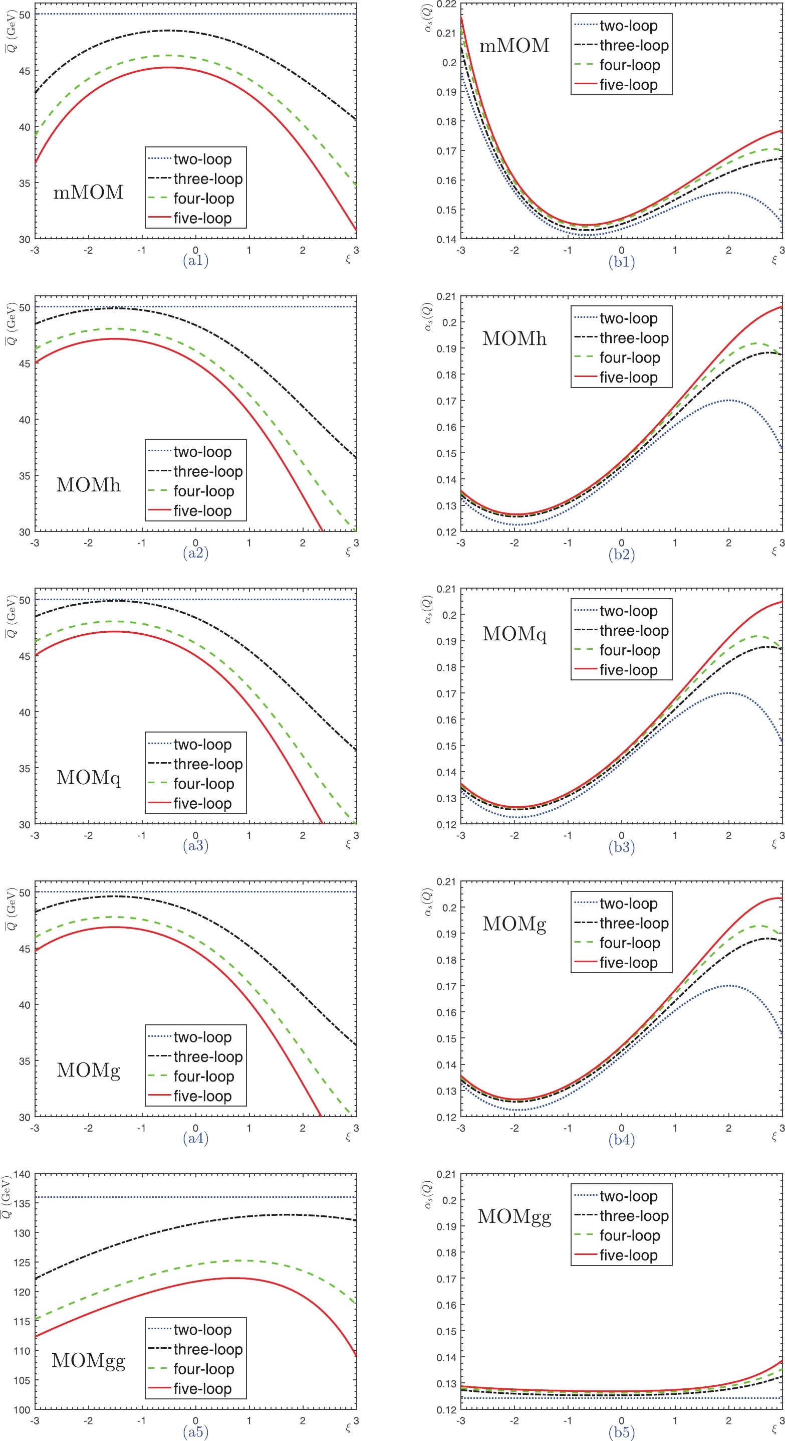
Figure 5. (color online) The PMC effective scales
$ \bar{Q} $ (left) and their corresponding coupling constants$ \alpha_s(\bar{Q}) $ (right) with respect to the gauge parameter ($ \xi $ ). Five asymmetric MOM schemes are adopted: mMOM, MOMh, MOMq, MOMg, and MOMgg. The dotted, dash-dot, dashed, and solid lines represent results for two-, three-, four-, and five-loop QCD corrections, respectively.Interestingly, under the MOMgg scheme, the effective coupling
$ \alpha_s(\bar{Q}) $ is also accurate at lower orders, and its value is almost gauge independent for$ |\xi^{\rm MOMgg}|\leqslant 1 $ ; this indicates that the gauge dependence of$ \bar{Q} $ is well compensated for by the gauge dependence of$ \Lambda^{\rm MOMgg}_{\rm QCD} $ . More explicitly, the asymptotic scales for various MOM schemes can be derived from$ \Lambda_{\overline{\rm MS}} $ by using the Celmaster–Gonsalves relation [3-7]. We present the ratios of$ {\Lambda_{\rm{MOM}}}/{\Lambda_{\overline{\rm{MS}}}} $ for$ n_f = 5 $ in Fig. 6, where the ratios for the three aforementioned symmetric MOM schemes are also presented. It is found that the asymptotic scales of the MOMg, MOMq, and MOMh schemes are identical; combining this with the similar values of$ \bar{Q} $ , we can explain the similar behaviors of$ \alpha_s(\bar{Q}) $ and$ \Gamma(H\to gg) $ under these schemes. Almost all of the ratios show an explicit gauge dependence; the only exception is the ratio of the MOMgg scheme, whose value is free of$ \xi^{\rm MOMgg} $ and fixed as$ e^{50/69}\approx 2.06 $ for$ n_f = 5 $ .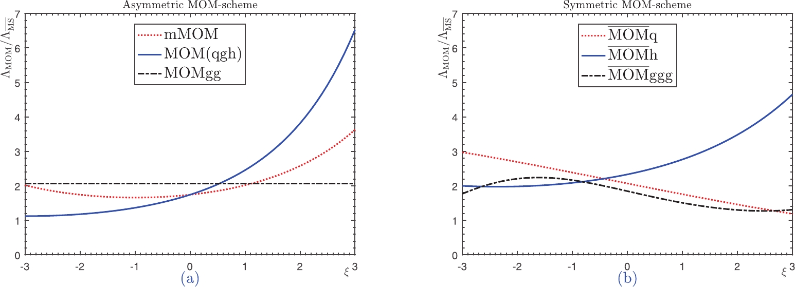
Figure 6. (color online) Gauge dependence of the ratio
$ \Lambda_{\rm{MOM}}/\Lambda_{\overline{\rm MS}} $ , obtained by varying the gauge parameter$ \xi = \xi^{\rm MOM} \in [-3,3] $ ,$ n_f = 5 $ . (a) The ratios for five asymmetric MOM schemes, where the asymptotic scales of the MOMg, MOMq, and MOMh schemes are identical and shown by the solid line; (b) the ratios for the three symmetric MOM-schemes. -
In Figs. 7-11, we present the total decay width
$ \Gamma (H \to gg) $ up to its two-, three-, four-, and five-loop levels before and after applying the PMC. The conventional renormalization scale dependence is estimated by varying$ \mu \in [M_H/4,4M_H] $ and becomes smaller when more loop terms are included; for example, the shaded bands become narrower under greater numbers of loop terms. This accords well with the results in the literature. Meanwhile, we can observe that the PMC predictions under various MOM schemes are scale-independent for any fixed order but become more accurate when more loop terms are included. Thus, the conventional renormalization scale uncertainty is eliminated by applying the PMC, which is consistent with the previous PMC examples considered in the literature. As mentioned in the Introduction, the scale independence of the PMC prediction is reasonable, since the determined scale$ \bar{Q} $ reflects the overall typical momentum flow of the process, which should be independent of the induced parameters.
Figure 7. (color online) Total decay width
$ \Gamma (H\to gg) $ with respect to the gauge parameter$ \xi=\xi^{\rm mMOM} $ under the mMOM scheme for two-, three-, four-, and five-loop levels, respectively. The dotted line denotes the conventional scale-setting approach using$ \mu = M_H $ , and the shaded band denotes its renormalization scale uncertainty, obtained by varying$ \mu \in [M_H/4,4M_H] $ . The solid line is the prediction for the PMC scale-setting, which is independent of the choice of renormalization scale.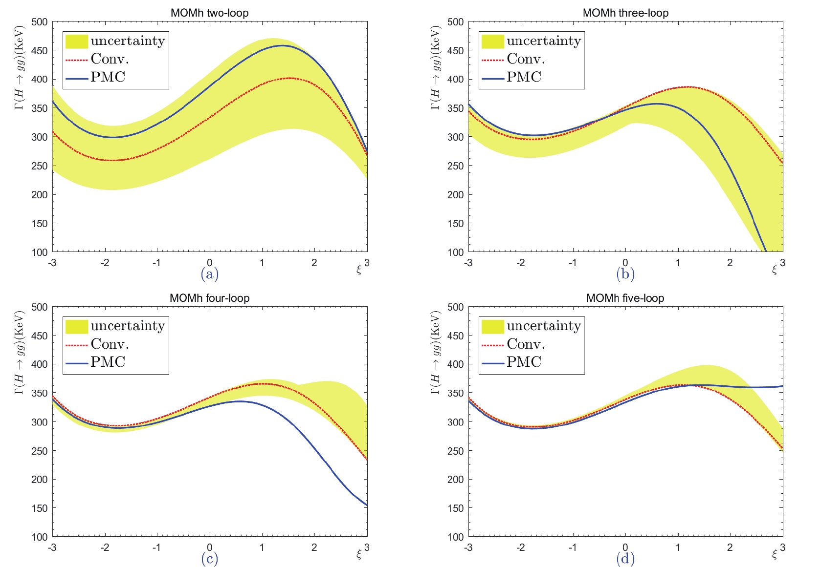
Figure 8. (color online) Total decay width
$ \Gamma (H\to gg) $ with respect to the gauge parameter$ \xi=\xi^{\rm MOMh} $ under the MOMh scheme for two-, three-, four-, and five-loop levels, respectively. The dotted line denotes the conventional scale-setting approach with$ \mu = M_H $ , and the shaded band shows its renormalization scale uncertainty, obtained by varying$ \mu \in [M_H/4,4M_H] $ . The solid line is the prediction for the PMC scale-setting, which is independent of the choice of renormalization scale.
Figure 9. (color online) Total decay width
$ \Gamma (H\to gg) $ with respect to the gauge parameter$ \xi=\xi^{\rm MOMq} $ under the MOMq scheme for two-, three-, four-, and five-loop levels, respectively. The dotted line denotes the conventional scale-setting approach with$ \mu = M_H $ , and the shaded band shows its renormalization scale uncertainty, obtained by varying$ \mu \in [M_H/4,4M_H] $ . The solid line is the prediction for the PMC scale-setting, which is independent of the choice of renormalization scale.
Figure 10. (color online) Total decay width
$ \Gamma (H\to gg) $ with respect to the gauge parameter$ \xi=\xi^{\rm MOMg} $ under the MOMg scheme for two-, three-, four-, and five-loop levels, respectively. The dotted line denotes the conventional scale-setting approach with$ \mu = M_H $ , and the shaded band shows its renormalization scale uncertainty, obtained by varying$ \mu \in [M_H/4,4M_H] $ . The solid line is the prediction for the PMC scale-setting, which is independent of the choice of renormalization scale.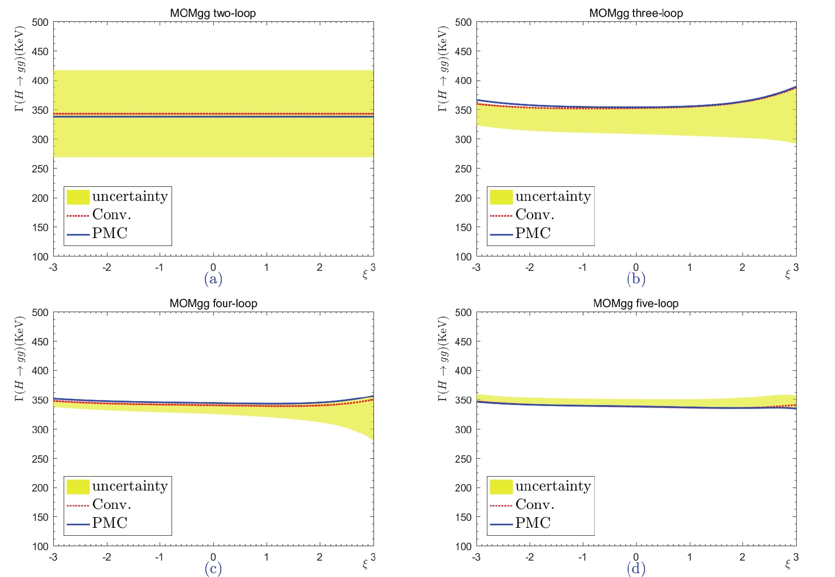
Figure 11. (color online) Total decay width
$ \Gamma (H\to gg) $ versus gauge parameter$ \xi = \xi^{\rm MOMgg} $ up to two-, three-, four-, and five-loop levels, respectively, under the MOMg scheme. The dotted line denotes the conventional scale-setting approach with$ \mu = M_H $ , and the shaded band shows its renormalization scale uncertainty by varying$ \mu \in [M_H/4,4M_H] $ . The solid line is the prediction for the PMC, which is independent of the choice of renormalization scale.Figures 7-11 show that the gauge dependence cannot be eliminated by including more higher-order terms, for both the conventional and PMC scale-setting approaches. More explicitly, the total decay widths of
$ H \to gg $ up to the five-loop level under the mMOM, MOMh, MOMq, MOMg, and MOMgg schemes are presented in Tables 1 and 2. The present prediction of$ \Gamma(H \to gg) $ by the ''LHC Higgs Cross-Section Working Group'' is approximately$ 335.4\; \rm{KeV} $ for$ M_H = 125.09 $ GeV③. In contrast to the dimensional-like schemes (which are gauge independent), gauge dependence is an intrinsic component of MOM schemes, and we cannot expect to eliminate it by including higher-order terms. As discussed in the Introduction, the MOM schemes have some advantages in dealing with the perturbative series; as will be shown below, the scheme independence of variance of MOM predictions can be greatly suppressed at higher orders. Thus, it is interesting to find which regions of$ \xi^{\rm MOM} $ present the most reliable MOM predictions. In accordance with the suggestions of Ref. [10], Figs. 7–11 show that the gauge dependence is relatively weak within the region of$ \xi^{\rm MOM} \in [-1,1] $ . As an exception, Fig. 11 indicates that at sufficently higher orders, the MOMgg prediction can be constant for a wide range of$ |\xi^{\rm MOMgg}| $ . Thus, of all the schemes considered, we prefer MOMgg. More explicitly, the coefficient functions$ C_{i\geq2} $ in Eq. (50) and$ r_{i\geq2,0} $ in Eq. (51) are power series of$ \xi^{\rm MOM} $ ; thus, a small magnitude (such as$ |\xi^{\rm MOM}|\leqslant 1 $ ) could result in a better convergence and steadier prediction over the change of$ \xi^{\rm MOM} $ ; this is why the Landau gauge (with$ \xi^{\rm MOM} = 0 $ ) is typically adopted in the literature [4]. Furthermore, we agree that a smaller value of$ |\xi^{\rm MOM}| $ is preferable for various MOM schemes. In the following discussion, we adopt$ \xi^{\rm MOM} \in [-1,1] $ .$ \xi^{\rm MOM} $ 

$ -3 $ 

$ -2 $ 

$ -1 $ 

0 1 2 3 $ \Gamma|^{\rm{mMOM}} $ 

627.3 398.7 338.5 337.7 350.1 336.9 273.6 $ \Gamma|^{\rm{MOMh}} $ 

341.3 291.5 301.8 337.7 363.2 338.1 252.5 $ \Gamma|^{\rm{MOMq}} $ 

341.3 291.4 301.8 337.7 363.3 338.1 252.1 $ \Gamma|^{\rm{MOMg}} $ 

341.1 291.4 301.8 337.7 363.2 337.9 251.2 $ \Gamma|^{\rm{MOMgg}} $ 

346.4 340.9 338.8 337.4 335.7 335.3 340.3 Table 1. Total decay width (unit: keV) of
$ H \to gg $ under the conventional scale-setting approach up to the five-loop level under the mMOM, MOMh, MOMq, MOMg, and MOMgg schemes. Typical gauge of conventional scale-setting approach. All other input parameters are set to their central values.$ \xi^{\rm MOM} $ 

$ -3 $ 

$ -2 $ 

$ -1 $ 

0 1 2 3 $ \Gamma|^{\rm{mMOM}}_{\rm PMC} $ 

590.9 389.8 333.4 332.8 344.3 327.7 249.8 $ \Gamma|^{\rm{MOMh}} $ 

335.8 288.2 298.2 332.8 360.3 360.7 361.4 $ \Gamma|^{\rm{MOMq}} $ 

335.8 288.2 298.2 332.9 360.2 359.2 352.6 $ \Gamma|^{\rm{MOMg}} $ 

335.5 288.0 298.1 332.7 360.1 360.2 347.5 $ \Gamma|^{\rm{MOMgg}} $ 

345.7 340.8 339.1 337.9 336.2 335.2 334.2 Table 2. Total decay width (unit: keV) of
$ H \to gg $ under PMC scale-setting approach up to the five-loop level under the mMOM, MOMh, MOMq, MOMg, and MOMgg schemes. Typical gauge of conventional scale-setting approach. All other input parameters are set to their central values.To more explicitly show how the scheme and scale dependence varies with the increasing orders under the conventional scale-setting approach, we obtain the following values:
$ \begin{split} \Gamma(H \to gg)|^{\rm{mMOM}, 2l}_{\rm{Conv.}} = 332.9{^{+25.9}_{-7.2}}\pm7.7\pm1.7{^{+77.7}_{-72.0}}\; \rm{keV}, \\ \Gamma(H \to gg)|^{\rm{mMOM}, 3l}_{\rm{Conv.}} = 350.6{^{+16.9}_{-5.0}}\pm8.4\pm1.8{^{+2.6}_{-33.4}}\; \rm{keV}, \\ \Gamma(H \to gg)|^{\rm{mMOM}, 4l}_{\rm{Conv.}} = 341.4{^{+12.7}_{-3.9}}\pm7.9\pm1.8{^{+1.1}_{-16.3}}\; \rm{keV}, \\ \Gamma(H \to gg)|^{\rm{mMOM}, 5l}_{\rm{Conv.}} = 337.7{^{+12.5}_{-3.8}}\pm7.7\pm1.7{^{+7.2}_{-1.4}}\; \rm{keV}. \end{split} $

$ \begin{split} \Gamma(H \to gg)|^{\rm{MOMh}, 2l}_{\rm{Conv.}} = 332.9{^{+57.0}_{-55.3}}\pm7.7\pm1.7{^{+77.7}_{-72.0}}\; \rm{keV}, \\ \Gamma(H \to gg)|^{\rm{MOMh}, 3l}_{\rm{Conv.}} = 350.6{^{+33.8}_{-42.0}}\pm8.4\pm1.8{^{+2.6}_{-33.4}}\; \rm{keV}, \\ \Gamma(H \to gg)|^{\rm{MOMh}, 4l}_{\rm{Conv.}} = 341.4{^{+24.1}_{-36.8}}\pm7.9\pm1.8{^{+1.1}_{-16.3}}\; \rm{keV}, \\ \Gamma(H \to gg)|^{\rm{MOMh}, 5l}_{\rm{Conv.}} = 337.7{^{+25.6}_{-35.9}}\pm7.7\pm1.7{^{+7.2}_{-1.4}}\; \rm{keV}. \end{split} $

$ \begin{split} \Gamma(H \to gg)|^{\rm{MOMq}, 2l}_{\rm{Conv.}} = 332.9{^{+57.0}_{-55.3}}\pm7.7\pm1.7{^{+77.7}_{-72.0}}\; \rm{keV}, \\ \Gamma(H \to gg)|^{\rm{MOMq}, 3l}_{\rm{Conv.}} = 350.2{^{+33.8}_{-42.0}}\pm8.4\pm1.8{^{+2.6}_{-33.3}}\; \rm{keV}, \\ \Gamma(H \to gg)|^{\rm{MOMq}, 4l}_{\rm{Conv.}} = 341.4{^{+24.2}_{-36.8}}\pm7.9\pm1.8{^{+1.0}_{-16.0}}\; \rm{keV}, \\ \Gamma(H \to gg)|^{\rm{MOMq}, 5l}_{\rm{Conv.}} = 337.7{^{+25.7}_{-35.9}}\pm7.7\pm1.7{^{+7.1}_{-1.4}}\; \rm{keV}. \end{split} $

$ \begin{split} \Gamma(H \to gg)|^{\rm{MOMg}, 2l}_{\rm{Conv.}} = 332.9{^{+57.0}_{-55.3}}\pm7.7\pm1.7{^{+77.7}_{-72.0}}\; \rm{keV}, \\ \Gamma(H \to gg)|^{\rm{MOMg}, 3l}_{\rm{Conv.}} = 350.4{^{+33.8}_{-42.0}}\pm8.4\pm1.8{^{+2.6}_{-33.4}}\; \rm{keV}, \\ \Gamma(H \to gg)|^{\rm{MOMg}, 4l}_{\rm{Conv.}} = 341.4{^{+24.2}_{-36.8}}\pm7.9\pm1.8{^{+1.0}_{-16.2}}\; \rm{keV}, \\ \Gamma(H \to gg)|^{\rm{MOMg}, 5l}_{\rm{Conv.}} = 337.7{^{+25.6}_{-35.9}}\pm7.7\pm1.7{^{+7.1}_{-1.4}}\; \rm{keV}. \end{split} $

$ \begin{split} \Gamma(H \to gg)|^{\rm{MOMgg}, 2l}_{\rm{Conv.}} = 342.7^{+0.0}_{-0.0}\pm8.1\pm1.8{^{+74.3}_{-74.0}}\; \rm{keV}, \\ \Gamma(H \to gg)|^{\rm{MOMgg}, 3l}_{\rm{Conv.}} = 352.2{^{+2.2}_{-0.5}}\pm8.5\pm1.8{^{+0.9}_{-44.4}}\; \rm{keV}, \\ \Gamma(H \to gg)|^{\rm{MOMgg}, 4l}_{\rm{Conv.}} = 339.8{^{+1.3}_{-1.3}}\pm7.8\pm1.8{^{+2.3}_{-14.8}}\; \rm{keV}, \\ \Gamma(H \to gg)|^{\rm{MOMgg}, 5l}_{\rm{Conv.}} = 337.4{^{+1.5}_{-1.7}}\pm7.7\pm1.7{^{+12.9}_{-0.7}}\; \rm{keV}. \end{split} $

The central values are for all input parameters to be set to their central values. Here,
$ nl $ ($ n = (2,···,5) $ ) represents the result up to the n-loop QCD correction, and "Conv." denotes the "conventional scale-setting approach." The first errors (superscript and subscript) indicate the gauge dependence, obtained by varying$ \xi^{\rm MOM} $ within the region$ [-1,1] $ (the central value is expressed in the Landau gauge,$ \xi^{\rm MOM} = 0 $ ); the second error is found by setting$ \Delta\alpha_s(M_Z) = \pm0.0011 $ ; the third error incorporates the Higgs mass uncertainty$ \Delta M_H = \pm 0.24\; \rm{GeV} $ ; and the final errors (superscript and subscript) are found by varying the renormalization scale$ \mu \in [M_H/4,4M_H] $ .Under the conventional scale-setting approach, the uncertainty attributable to
$ \Delta\alpha_s(M_Z) $ is approximately 4% for all orders. The uncertainty attributable to the Higgs mass$ \Delta M_H = 0.24\; \rm{GeV} $ is approximately 1% for all orders. The uncertainties attributable to the choice of gauge parameter and renormalization scale are somewhat larger. By taking$ \xi^{\rm MOM}\in[-1,1] $ , the total decay width$ \Gamma(H \to gg)|^{\rm mMOM}_{\rm Conv.} $ is varied by approximately 10%, 6%, 5%, and 5% for$ n = 2,3,4,5 $ , respectively. The total decay widths$ \Gamma(H \to gg)|^{\rm MOMh, MOMq, MOMg}_{\rm Conv.} $ behave similarly; they vary by about 34%, 22%, 18%, and 18% for$ n = 2,3,4,5 $ , respectively. The total decay width$ \Gamma(H \to gg)|^{\rm MOMgg}_{\rm Conv.} $ is free of gauge dependence at the two-loop level, and it varies by about 1% for$ n = 3,4,5 $ . Thus, the gauge dependence of the MOMgg scheme is smallest. By taking$ \mu\in [M_H/4,4M_H] $ , the total decay width for the mMOM, MOMh, MOMq, and MOMg schemes can be seen to behave similarly; it varies by approximately 45%, 10%, 5%, and 3% for$ n = 2,3,4,5 $ , respectively. The total decay width$ \Gamma(H \to gg)|^{\rm MOMgg}_{\rm Conv.} $ is changed by about 43%, 13%, 5%, and 4% for$ n = 2,3,4,5 $ , respectively. Thus, by including more loop terms, the renormalization scale error can be decreased.After applying the PMC, the renormalization scale dependence is removed exactly, and we have
$ \begin{split} \Gamma(H \to gg)|^{\rm{mMOM}, 2l}_{\rm{PMC}} & = 386.7{^{+29.4}_{-8.3}}\pm10.0\pm1.9\; \rm{keV}, \\ \Gamma(H \to gg)|^{\rm{mMOM}, 3l}_{\rm{PMC}} & = 345.9{^{+7.2}_{-3.0}}\pm8.1\pm1.8\; \rm{keV}, \\ \Gamma(H \to gg)|^{\rm{mMOM}, 4l}_{\rm{PMC}} & = 326.2{^{+4.6}_{-2.4}}\pm6.9\pm1.7\; \rm{keV}, \\ \Gamma(H \to gg)|^{\rm{mMOM}, 5l}_{\rm{PMC}} & = 332.8{^{+11.6}_{-3.7}}\pm7.3\pm1.7\; \rm{keV}. \end{split} $

$ \begin{split} \Gamma(H \to gg)|^{\rm{MOMh}, 2l}_{\rm{PMC}} &= 386.7{^{+62.8}_{-66.0}}\pm10.0\pm1.9\; \rm{keV}, \\ \Gamma(H \to gg)|^{\rm{MOMh}, 3l}_{\rm{PMC}} &= 345.9{^{+10.7}_{-33.1}}\pm8.1\pm1.8\; \rm{keV}, \\ \Gamma(H \to gg)|^{\rm{MOMh}, 4l}_{\rm{PMC}} &= 326.2{^{+8.2}_{-28.2}}\pm6.9\pm1.7\; \rm{keV}, \\ \Gamma(H \to gg)|^{\rm{MOMh}, 5l}_{\rm{PMC}} &= 332.8{^{+27.5}_{-34.6}}\pm7.3\pm1.7\; \rm{keV}. \end{split} $

$ \begin{split} \Gamma(H \to gg)|^{\rm{MOMq}, 2l}_{\rm{PMC}} &= 386.7{^{+62.8}_{-66.0}}\pm10.0\pm1.9\; \rm{keV}, \\ \Gamma(H \to gg)|^{\rm{MOMq}, 3l}_{\rm{PMC}} &= 345.6{^{+10.8}_{-33.2}}\pm8.1\pm1.8\; \rm{keV}, \\ \Gamma(H \to gg)|^{\rm{MOMq}, 4l}_{\rm{PMC}} &= 326.5{^{+8.4}_{-28.3}}\pm6.9\pm1.7\; \rm{keV}, \\ \Gamma(H \to gg)|^{\rm{MOMq}, 5l}_{\rm{PMC}} &= 332.9{^{+27.4}_{-34.7}}\pm7.3\pm1.7\; \rm{keV}. \end{split} $

$ \begin{split} \Gamma(H \to gg)|^{\rm{MOMg}, 2l}_{\rm{PMC}} &= 386.7{^{+62.8}_{-66.0}}\pm10.0\pm1.9\; \rm{keV}, \\ \Gamma(H \to gg)|^{\rm{MOMg}, 3l}_{\rm{PMC}} &= 345.8{^{+10.5}_{-33.0}}\pm8.1\pm1.8\; \rm{keV}, \\ \Gamma(H \to gg)|^{\rm{MOMg}, 4l}_{\rm{PMC}} &= 326.0{^{+8.0}_{-28.1}}\pm6.8\pm1.7\; \rm{keV}, \\ \Gamma(H \to gg)|^{\rm{MOMg}, 5l}_{\rm{PMC}} &= 332.7{^{+27.5}_{-34.6}}\pm7.3\pm1.7\; \rm{keV}. \end{split} $

$ \begin{split} \Gamma(H \to gg)|^{\rm{MOMgg}, 2l}_{\rm{PMC}} &= 337.8^{+0.0}_{-0.0}\pm7.9\pm1.7\; \rm{keV}, \\ \Gamma(H \to gg)|^{\rm{MOMgg}, 3l}_{\rm{PMC}} &= 353.6{^{+1.7}_{-0.1}}\pm8.6\pm1.8\; \rm{keV}, \\ \Gamma(H \to gg)|^{\rm{MOMgg}, 4l}_{\rm{PMC}} &= 343.6{^{+1.3}_{-1.1}}\pm8.1\pm1.8\; \rm{keV}, \\ \Gamma(H \to gg)|^{\rm{MOMgg}, 5l}_{\rm{PMC}} &= 337.9{^{+1.2}_{-1.7}}\pm7.7\pm1.8\; \rm{keV}. \end{split} $

As seen for the results obtained under the conventional scale-setting approach, the uncertainties caused by
$ \Delta\alpha_s(M_Z) $ and$ \Delta M_H $ are small, approximately 4% and 1%, respectively. However, the uncertainties caused by different choices of the gauge parameter are still sizable for various MOM schemes. For example, by taking$ \xi^{\rm MOM}\in[-1,1] $ , the total decay width$ \Gamma(H \to gg)|^{\rm mMOM}_{\rm PMC} $ is changed by approximately 10%, 3%, 2%, and 5% for$ n = 2,3,4,5 $ , respectively. The total decay widths$ \Gamma(H \to gg)|^{\rm MOMh, MOMq, MOMg}_{\rm PMC} $ behave similarly; they vary by approximately 33%, 12%, 11%, and 19% for$ n = 2,3,4,5 $ , respectively; the total decay width$ \Gamma(H \to gg)|^{\rm MOMgg}_{\rm PMC} $ is almost independent of the choice of gauge parameter; it changes by less than 1% for$ n = 3,4,5 $ .Generally, when using the estimated scale, the convergence of the conventional pQCD series varies considerably under different choices of the renormalization scale, due to the mismatching between the perturbative coefficient and the
$ \alpha_s $ -value at the same order. For example, a relatively sizeable scale uncertainty is found for each term of the pQCD series of$ \Gamma(H\to gg) $ [30, 31]; thus, even if a superior convergence can be acheived by choosing a proper scale④, we cannot determine whether such a choice leads to the correct pQCD prediction. On the other hand, by applying the PMC, the scale-independent coupling$ \alpha_s(\bar{Q}) $ can be determined; combining this with the scale-invariant conformal coefficients, we can obtain the intrinsic perturbative nature of the pQCD series. By defining a K factor as$ K = \Gamma(H \to gg)/$ $\Gamma(H \to gg)|_{\rm{Born}} $ , we can obtain the relative significance of higher-order terms with respect to the leading-order terms. More explicitly, under the Landau gauge (with$ \xi^{\rm MOM} = 0 $ ), we obtain$ K^{\rm{mMOM}} \simeq 1.07 = 1+0.31-0.17-0.08+0.01, $

(56) $ K^{\rm{MOMh}} \simeq 1.07 = 1+0.31-0.17-0.08+0.01, $

(57) $ K^{\rm{MOMq}} \simeq 1.07 = 1+0.31-0.17-0.08+0.01, $

(58) $ K^{\rm{MOMg}} \simeq 1.06 = 1+0.31-0.17-0.09+0.01, $

(59) $ K^{\rm{MOMgg}} \simeq 1.45 = 1+0.53+0.04-0.08-0.04. $

(60) These results exhibit a satisfactorily convergent behavior for
$ \Gamma(H\to gg) $ , especially for the mMOM, MOMh, MOMq, and MOMg schemes. As seen for the total decay width, the K factor is gauge dependent. By varying$ \xi^{\rm MOM}\in[-1,1] $ , we obtain$ K^{\rm{mMOM}} = 1.07{^{+0.03}_{-0.10}} $ ,$ K^{\rm{MOMh}} =$ $ 1.07{^{+0.12}_{-0.19}} $ ,$ K^{\rm{MOMq}} = 1.07{^{+0.12}_{-0.19}} $ ,$ K^{\rm{MOMg}} = 1.06{^{+0.12}_{-0.19}} $ , and$ K^{\rm{MOMgg}} = 1.45{^{+0.00}_{-0.02}} $ .One final remark: We typially wish to know the magnitude of the ''unknown" high-order pQCD corrections. The conventional error estimates obtained by varying the scale over a certain range are usually treated as such an estimation; however, this is an unreliable method because it partly estimates the non-conformal contribution and does not estimate the conformal one. In contrast, after applying the PMC, the correct momentum flow of the process (and hence the correct
$ \alpha_s $ -value) is fixed by the RGE and cannot be varied; otherwise, the RGI will be explicitly broken, leading to an unreliable prediction. As a conservative estimate of the magnitude of the unknown perturbative contributions to the PMC series, it is helpful to use the magnitude of the last known term as the contribution of the unknown perturbative term [69]. In the present case, we adopt$ \pm |r_{5,0}a^6_s(\bar{Q})| $ as the estimation of the unknown$ {\cal O}(\alpha_s^6) $ contribution; it is$ \pm 3.1 $ keV for the mMOM, MOMh, MOMq, and MOMg schemes, and$ \pm 9.3 $ keV for the MOMgg scheme. -
In addition to the asymmetric MOM schemes, several symmetric MOM schemes have been suggested in the literature. In the original symmetric MOM scheme [4], the triple-gluon vertex function
$ \Gamma_{\mu \nu \rho}^{a b c}(k, p, l) $ was defined as the value at the symmetric point$ k^2 = p^2 = l^2 = -\mu^2 $ ; that is, the Feynman diagram of the vertex is identical to that presented in Fig. 4, though the three external momenta ($ q, -q, 0 $ ) shown there should be replaced by the current ($ k, p, l $ ). Similarly, the ghost-gluon vertex function$ \tilde{\Gamma}_{\mu}^{a b c}(k, p, l) $ and quark-gluon vertex function$ \Lambda^a_{\mu,ij}(k, p, l) $ can also be defined at the symmetric point$ k^2 = p^2 = l^2 = -\mu^2 $ [32, 88, 89]. For simplicity, we label these symmetric MOM schemes (defined at the triple-, ghost-, and quark-gluon vertices) as the$ {\overline {\rm{MOM}}}{\rm{ggg}} $ ,$ {\overline{\rm{MOM}}}{\rm{h}} $ , and$ {\overline{\rm{MOM}}}{\rm{q}} $ schemes, respectively. Using the relations expressed in Eqs. (21) and (22), along with the three-loop vertex functions found under the$ \overline{\rm MS} $ scheme (collected in Ref. [32]), we obtain expressions for the strong couplings and gauge parameters of those symmetric MOM schemes up to the three-loop level [89]⑤. Then, using those expressions, we can obtain the pQCD series for$ \Gamma(H \to gg) $ under the$ {\overline{\rm{MOM}}} {\rm{ggg}}$ ,$ {\overline{\rm{MOM}}} {\rm{h}}$ , and$ {\overline{\rm{MOM}}} {\rm{q}}$ schemes up to the three-loop level.After applying the conventional and PMC scale-setting approaches, we obtain
$ \begin{split} \Gamma(H \to gg)|^{\overline{\rm{MOM}ggg}, 2l}_{\rm{Conv.}} &= 336.2{^{+36.2}_{-26.9}}\pm7.8\pm1.7{^{+76.7}_{-72.7}}\; \rm{keV}, \\ \Gamma(H \to gg)|^{\overline{\rm{MOM}ggg}, 3l}_{\rm{Conv.}} &= 349.5{^{+24.6}_{-14.5}}\pm8.3\pm1.8{^{+1.9}_{-32.1}}\; \rm{keV}, \\ \Gamma(H \to gg)|^{\overline{\rm{MOM}h}, 2l}_{\rm{Conv.}} &= 350.0{^{+29.3}_{-26.1}}\pm8.4\pm1.8{^{+70.5}_{-75.4}}\; \rm{keV}, \\ \Gamma(H \to gg)|^{\overline{\rm{MOM}h}, 3l}_{\rm{Conv.}} &= 351.6{^{+20.2}_{-20.1}}\pm8.4\pm1.8{^{+0.2}_{-55.9}}\; \rm{keV}, \\ \Gamma(H \to gg)|^{\overline{\rm{MOM}q}, 2l}_{\rm{Conv.}} &= 342.9{^{+42.8}_{-24.0}}\pm8.1\pm1.8{^{+74.2}_{-74.1}}\; \rm{keV}, \\ \Gamma(H \to gg)|^{\overline{\rm{MOM}q}, 3l}_{\rm{Conv.}} &= 342.5{^{+32.2}_{-14.4}}\pm8.0\pm1.8{^{+0.9}_{-35.0}}\; \rm{keV}, \end{split} $

and
$ \begin{split} \Gamma(H \to gg)|^{\overline{\rm{MOM}ggg}, 2l}_{\rm{PMC}} &= 291.5{^{+30.1}_{-22.6}}\pm6.1\pm1.5\; \rm{keV}, \\ \Gamma(H \to gg)|^{\overline{\rm{MOM}ggg}, 3l}_{\rm{PMC}} &= 323.6{^{+26.0}_{-14.2}}\pm7.1\pm1.7\; \rm{keV}, \\ \Gamma(H \to gg)|^{\overline{\rm{MOM}h}, 2l}_{\rm{PMC}} &= 402.2{^{+30.9}_{-29.8}}\pm10.8\pm2.0\; \rm{keV}, \\ \Gamma(H \to gg)|^{\overline{\rm{MOM}h}, 3l}_{\rm{PMC}} &= 332.5{^{+6.9}_{-11.1}}\pm7.3\pm1.7\; \rm{keV}, \\ \Gamma(H \to gg)|^{\overline{\rm{MOM}q}, 2l}_{\rm{PMC}} &= 396.1{^{+49.1}_{-26.9}}\pm10.5\pm2.0\; \rm{keV},\\ \Gamma(H \to gg)|^{\overline{\rm{MOM}q}, 3l}_{\rm{PMC}} &= 332.5{^{+25.4}_{-8.7}}\pm7.4\pm1.7\; \rm{keV}. \end{split} $

The central values are for all input parameters to be their central values, and the errors arise through employing the same input-parameter selection method as that for asymmetric schemes.
In Fig. 12, we present the PMC effective scales
$ \bar{Q} $ and corresponding coupling constants$ \alpha_s(\bar{Q}) $ for$ \Gamma (H\to gg) $ under three symmetric MOM schemes Fig. 12. The total decay widths$ \Gamma (H\to gg) $ with respect to the gauge parameter for three symmetric MOM schemes are presented in Fig. 13. Similar to the case of the asymmetric MOM scheme, the gauge dependence cannot be suppressed by eliminating the scale dependence. More explicitly, we present the total decay width$ \Gamma(H \to gg) $ for several typical gauge parameters in Table 3.$ \xi^{\rm MOM} $ 

−3 −2 −1 0 1 2 3 $ \Gamma|^{\rm{\overline{MOM}ggg}}_{\rm Conv.} $ 

101.1 293.9 374.1 349.5 335.3 357.2 395.9 $ \Gamma|^{\rm{\overline{MOM}h}}_{\rm Conv.} $ 

404.3 340.1 333.3 351.6 370.0 363.9 322.6 $ \Gamma|^{\rm{\overline{MOM}q}}_{\rm Conv.} $ 

472.3 420.7 374.7 342.5 328.2 335.2 370.6 $ \Gamma|^{\rm{\overline{MOM}ggg}}_{\rm PMC} $ 

107.0 287.3 349.6 323.6 309.4 323.8 336.5 $ \Gamma|^{\rm{\overline{MOM}h}}_{\rm PMC} $ 

395.2 331.5 321.5 332.5 339.2 319.6 267.5 $ \Gamma|^{\rm{\overline{MOM}q}}_{\rm PMC} $ 

434.5 394.7 357.8 332.5 323.9 336.5 378.7 Table 3. Gauge dependence of the total decay width (unit: keV) for
$ H \to gg $ up to the three-loop level under the$ \rm{\overline{MOM}ggg} $ ,$ \rm{\overline{MOM}h} $ , and$ \rm{\overline{MOM}q} $ schemes, before and after applying the PMC. The other input parameters are set as their central values.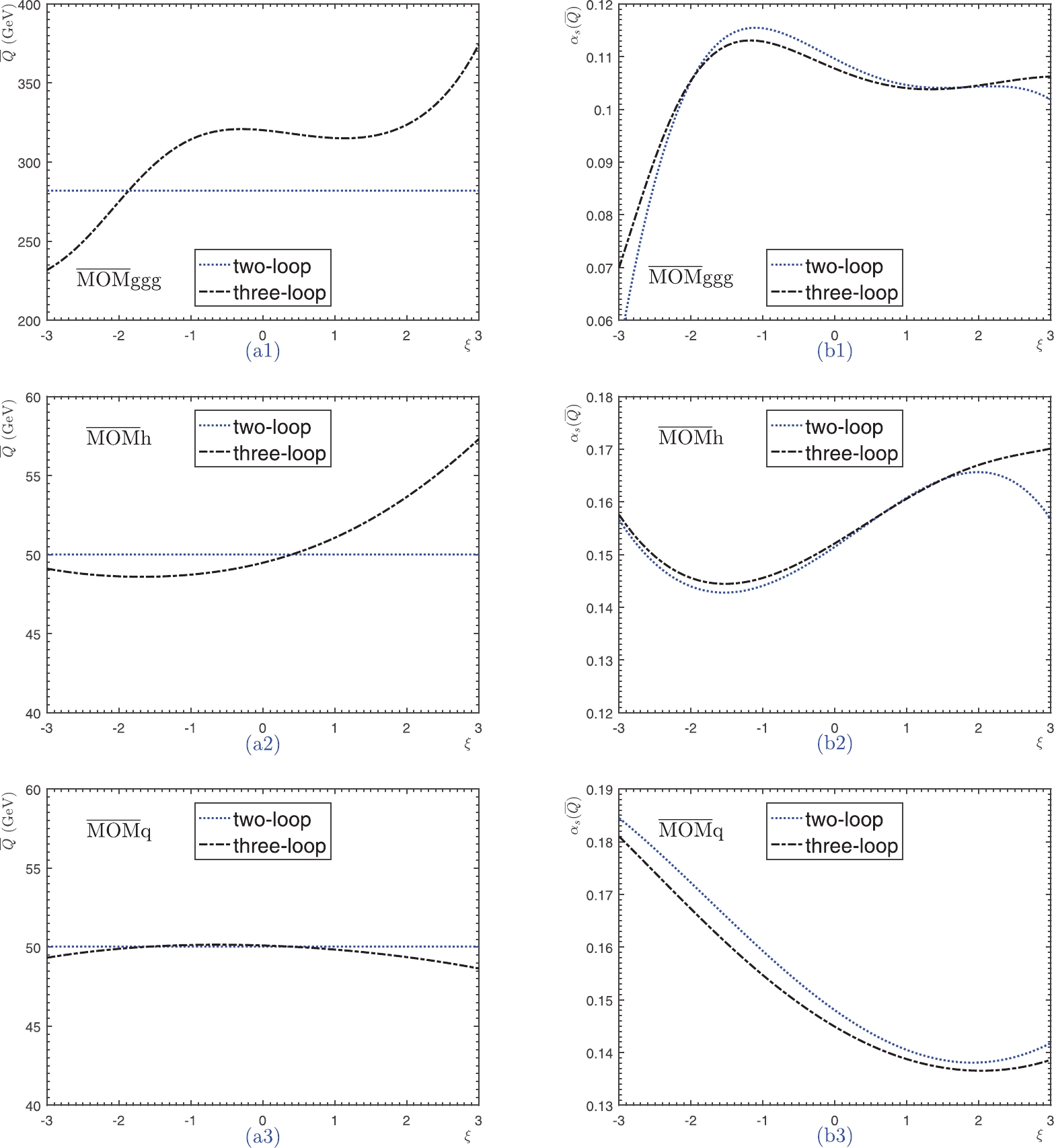
Figure 12. (color online) The PMC effective scales
$ \bar{Q} $ (left) and their corresponding coupling constants$ \alpha_s(\bar{Q}) $ (right) with respect to the gauge parameter ($ \xi $ ) of$ \Gamma (H\to gg) $ . Three symmetric MOM schemes ($ \rm{\overline{MOM}ggg} $ ,$ \rm{\overline{MOM}h} $ , and$ \rm{\overline{MOM}q} $ ) are adopted. The dotted and dash-dot lines denote the results up to the two- and three-loop QCD corrections, respectively.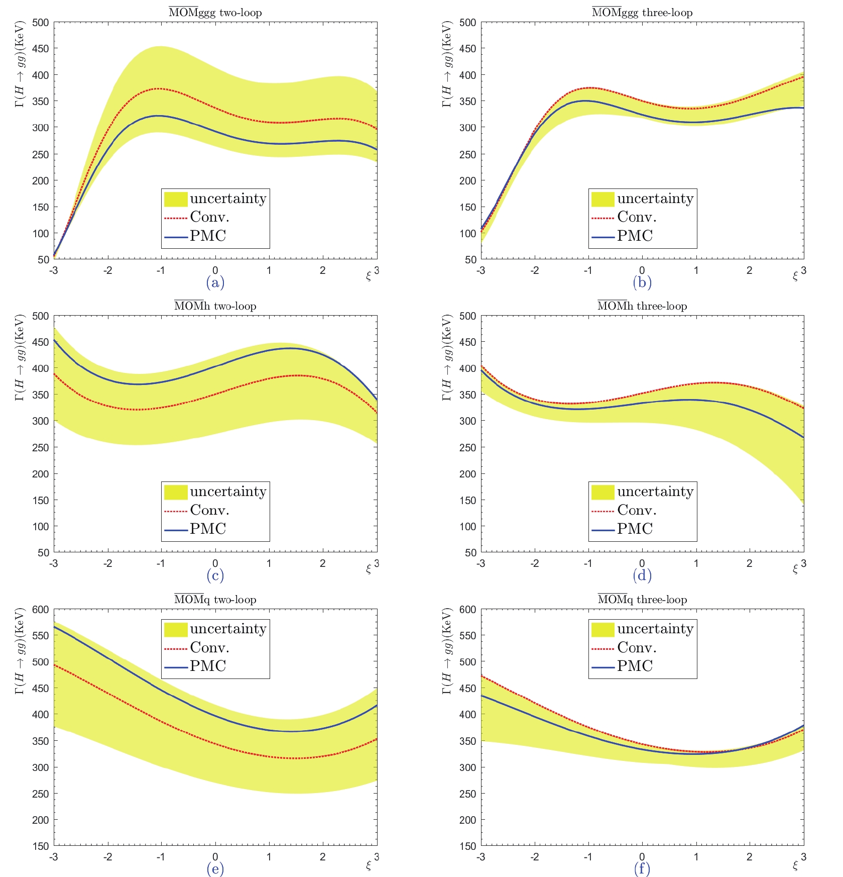
Figure 13. (color online) Total decay width
$ \Gamma (H\to gg) $ with respect to the gauge parameter ($ \xi $ ) up to the two- and three-loop levels under three symmetric MOM schemes. The dotted line represents the conventional scale-setting approach with$ \mu = M_H $ , and the shaded band shows its renormalization scale uncertainty, obtained by varying$ \mu \in [M_H/4,4M_H] $ . The solid line is the PMC prediction, which is independent of the choice of renormalization scale. -
In this paper, we presented a detailed discussion on the gauge dependence of the total decay width
$ \Gamma(H \to gg) $ up to the five-loop level under various MOM schemes. Our main results are as follows:● The gauge and renormalization scale dependence under the MOM schemes are two different entities. Figs. 7-11 show that under the conventional scale-setting approach, the total scale dependence of
$ \Gamma(H \to gg) $ can be greatly suppressed when more loop terms are known, due to the correlations of scale dependence among different orders; however, the gauge dependence of the pQCD approximant behaves differently for different choices of scale and MOM scheme. After applying the PMC, the conventional renormalization scale dependence can be eliminated; however, the gauge dependence of the MOM scheme remains and cannot be suppressed by including more loop terms. The gauge dependence may become even larger at higher orders. Thus, gauge dependence is an intrinsic property of MOM schemes. Despite this limitation, MOM schemes offer several advantages in dealing with pQCD predictions, as explained in the Introduction. Of all the MOM schemes, the gauge dependence of$ \Gamma(H\to gg) $ under the$ \rm{MOMgg} $ scheme is the smallest (below ±1%). In this sense, the MOMgg scheme can be considered the ideal type of MOM scheme.● By applying the PMC, the scale-independent effective momentum flow (
$ \bar{Q} $ ) of the process can be fixed using the RGE; as shown in Figs. 5 and 12, it differs between MOM schemes, which ensures the scheme independence of the pQCD predictions [40]. For example, if we set$ \xi^{\rm MOM}\in[-3, 3] $ , then the effective scale$ \bar{Q} $ is$ \sim [31, 45] $ GeV for the mMOM scheme,$ \sim[25, 47] $ GeV for the MOMh, MOMq, and MOMg schemes, and$ \sim [109,122] $ GeV for the MOMgg scheme. If we set$ \xi^{\rm MOM} $ to within a smaller allowable region$ [-1, 1] $ , the effective scale$ \bar{Q} $ becomes$ \sim [43, 45] $ GeV for the mMOM scheme,$ \sim[40, 47] $ GeV for the MOMh, MOMq, and MOMg schemes, and$ \sim [119,122] $ GeV for the MOMgg scheme. The small differences of$ \bar{Q} $ observed for$ \xi^{\rm MOM}\in[-1, 1] $ can be further compensated for by the differences of asymptotic scale, which results in a weaker gauge dependence of$ \Gamma(H\to gg) $ for$ \xi^{\rm MOM} \in [-1,1] $ .● Applying the PMC eliminates the renormalization scale ambiguity; hence, a more accurate pQCD prediction for
$ \Gamma(H\to gg) $ can be achieved. The uncertainties caused by$ \Delta\alpha_s(M_Z) $ and$ \Delta M_H $ are found to be small, approximately 4% and 1%, respectively. By taking$ \xi^{\rm MOM}\in[-1,1] $ , the total decay width$ \Gamma(H \to gg)|^{\rm mMOM}_{\rm PMC} $ is changed by about 10%, 3%, 2%, and 5% for$ n = 2,3,4,5 $ , respectively; the total decay widths$ \Gamma(H \to gg)|^{\rm MOMh, MOMq, MOMg}_{\rm PMC} $ behave similarly, changing by approximately 33%, 12%, 11%, and 19% for$ n = 2,3,4,5 $ , respectively; the total decay width$ \Gamma(H \to gg)|^{\rm MOMgg}_{\rm PMC} $ is almost independent of the choice of gauge parameter, and it changes by only ~1% for$ n = 3,4,5 $ . By summing all the aforementioned errors in quadrature, we obtain the five-loop predictions of$ \Gamma(H\to gg) $ under five asymmetric MOM schemes,$\Gamma(H \to gg)|^{\rm{mMOM}}_{\rm{PMC}} = 332.8^{+13.8}_{-8.4}\; \rm{keV}, $

(61) $ \begin{array}{l} \Gamma(H \to gg)|^{\rm{MOMh}}_{\rm{PMC}} = 332.8^{+28.5}_{-35.6}\; \rm{keV}, \end{array} $

(62) $ \begin{array}{l} \Gamma(H \to gg)|^{\rm{MOMq}}_{\rm{PMC}} = 332.9^{+28.4}_{-35.5}\; \rm{keV}, \end{array} $

(63) $ \begin{array}{l} \Gamma(H \to gg)|^{\rm{MOMg}}_{\rm{PMC}} = 332.7^{+28.4}_{-35.4}\; \rm{keV}, \end{array} $

(64) $ \begin{array}{l} \Gamma(H \to gg)|^{\rm{MOMgg}}_{\rm{PMC}} = 337.9^{+7.6}_{-7.7}\; \rm{keV}. \end{array} $

(65) The MOMgg decay width has the smallest net error, due to the small gauge dependence. The Higgs decay width
$ \Gamma (H\to gg) $ is found to vary weakly according to the choice of MOM scheme, which is consistent with RGI. Such small differences (less than ~1%) between the different schemes could be attributed to the unknown higher-order terms; e.g., the unknown N$ ^4 $ LL and higher-order terms in the PMC scale$ \bar{Q} $ 's perturbative series [71]. For example, from Eq. (53), we can see that if we treat$ \pm |\lambda_{3} a^3(Q)| $ as the estimated contribution of the unknown N$ ^4 $ LL-term of$ \bar{Q} $ , the change of the total decay width$ \Delta\Gamma(H \to gg) $ well explains the disparities between the total decay widths for different schemes; e.g.,$ \Delta\Gamma(H \to gg)|_{\rm{PMC}}\simeq \pm2.8 $ keV for all the MOM schemes.● The pQCD convergence of the conventional series varies greatly under different choices of the renormalization scale, due to the mismatch between the perturbative coefficient and
$ \alpha_s $ -value at the same order. Thus, it is improper to use the conventional series to predict the unknown terms. On the other hand, after applying the PMC, the scale-independent coupling$ \alpha_s(\bar{Q}) $ can be determined; combining this with the scale-invariant conformal coefficients, we can deduce the intrinsic perturbative nature of the pQCD series and more reliably predict unknown terms. Using the known five-loop prediction of$ \Gamma(H \to gg) $ as an explicit example, if we choose$ \pm |r_{5,0}a^6_s(\bar{Q})| $ as a conservative estimate of the unknown six-loop prediction, we obtain the$ {\cal O}(\alpha_s^6) $ contribution as$ \pm 3.1 $ keV for the mMOM, MOMh, MOMq, and MOMg schemes, and$ \pm 9.3 $ keV for the MOMgg scheme. -
Eq. (18) shows that for any scheme R, we have
$ \begin{array}{l} Z_a^R = \dfrac{1}{Z_3^R}\Bigg(\frac{\tilde{Z}_1^R}{\tilde{Z}_3^R}\Bigg)^2, \end{array}\tag{A1} $

(A1) then, we obtain
$ \begin{split} \frac{Z_a^{\overline{\rm{MS}}}}{Z_a^{\rm{mMOM}}} =& \frac{Z_3^{\rm{mMOM}}}{Z_3^{\overline{\rm{MS}}}}\Bigg(\frac{\tilde{Z}_1^{\overline{\rm{MS}}}}{\tilde{Z}_1^{\rm{mMOM}}}\Bigg)^2 \Bigg(\frac{\tilde{Z}_3^{\rm{mMOM}}}{\tilde{Z}_3^{\overline{\rm{MS}}}}\Bigg)^2 \\ =& \frac{Z_3^{\rm{mMOM}}}{Z_3^{\overline{\rm{MS}}}}\Bigg(\frac{\tilde{Z}_3^{\rm{mMOM}}}{\tilde{Z}_3^{\overline{\rm{MS}}}}\Bigg)^2. \end{split}\tag{A2} $

(A2) Meanwhile, Eq. (12) leads to
$ \frac{Z_3^{\rm{mMOM}}}{Z_3^{\overline{\rm{MS}}}} = \frac{1+\Pi_A^{\rm{mMOM}}}{1+\Pi_A^{\overline{\rm{MS}}}}, \tag{A3} $

(A3) and Eq. (13) leads to
$ \frac{\tilde{Z}_3^{\rm{mMOM}}}{\tilde{Z}_3^{\overline{\rm{MS}}}} = \frac{1+\tilde{\Pi}_c^{\rm{mMOM}}}{1+\tilde{\Pi}_c^{\overline{\rm{MS}}}}.\tag{A4} $

(A4) At the subtraction point
$ q^2 = -\mu^2 $ , Eqs. (23) and (24) lead to$ \begin{split} \frac{Z_3^{\rm{mMOM}}}{Z_3^{\overline{\rm{MS}}}} =& \frac{1}{1+\Pi_A^{\overline{\rm{MS}}}}, \\ \Bigg(\frac{\tilde{Z}_3^{\rm{mMOM}}}{\tilde{Z}_3^{\overline{\rm{MS}}}}\Bigg)^2 =& \frac{1}{(1+\tilde{\Pi}_c^{\overline{\rm{MS}}})^2}. \end{split}\tag{A5} $

(A5) Substituting Eqs. (A2) and (A5) into Eq. (22), we obtain Eqs. (36) and (26), as required.
-
In this appendix, we provide the perturbative transformations from the strong couplings and gauge parameters of a specific MOM scheme to those of the
$ \overline{\rm MS} $ scheme. For convenience, we use the notations$ (\overline{a}, \overline{\xi}) $ and$ (a, \xi) $ to represent$ (a^{\overline{\rm{MS}}}, \xi^{\overline{\rm{MS}}}) $ and$ (a^{\rm{MOM}}, \xi^{\rm{MOM}}) $ , respectively. The transformations were first considered in Ref. [4] and then improved in Ref. [80]. Here, for self-consistency and in light of our present purposes, we present a more detailed and one-order higher derivation than that of Ref. [80].Generally, the strong couplings and gauge parameters of a MOM scheme can be expanded over those of the
$ \overline{\rm MS} $ scheme. Up to the presently known order, and to suit the needs of our present discussion, we have$ a = \overline{a}+\sum\limits _{i = 1}^4 \phi_{i}(\overline{\xi})\overline{a}^{i+1}+\mathcal{O}(\overline{a}^6), \tag{B1}$

(B1) $ \xi = \overline{\xi}\bigg(1+\sum\limits _{n = 1}^3\psi_{n}(\overline{\xi})\overline{a}^{n}+\mathcal{O}(\overline{a}^4)\bigg)\; . \tag{B2} $

(B2) Conversely, we have
$ \overline{a} = &a+\sum\limits _{n = 1}^4 b_{n}(\xi)a^{n+1}+\mathcal{O}(a^6), \tag{B3} $

(B3) $ \overline{\xi} = \xi \bigg(1+\sum\limits _{n = 1}^3\chi_{n}(\xi )a^{n}+\mathcal{O}(a^4)\bigg). \tag{B4} $

(B4) These two expansions (B3) and (B4) are important for transforming the known
$ \overline{\rm MS} $ perturbative series of a physical observable into the one expressed under a certain MOM scheme.Our task is to derive the coefficients
$ b_i(\xi) $ and$ \chi_i(\xi) $ from the known ones$ \phi_i(\overline{\xi}) $ and$ \psi_i(\overline{\xi}) $ . To this end, we first perform the following Taylor expansions:$ \phi_{i}(\overline{\xi}) = \sum\limits_{n = 0}^\infty \frac{{\rm d}^{n}\phi_{i}(\xi)}{n! {\rm d}\xi^{n}}(\overline{\xi}-\xi)^{n},i = 1,2,3,4\ldots, \tag{B5} $

(B5) $ \psi_{j}(\overline{\xi}) = \sum\limits_{n = 0}^\infty \frac{{\rm d}^{n}\psi_{j}(\xi)}{n! {\rm d}\xi^{n}}(\overline{\xi}-\xi)^{n},j = 1,2,3\ldots, \tag{B6} $

(B6) where
$ \begin{array}{l} \overline{\xi}-\xi = \xi\bigg(\chi_1(\xi)a+\chi_2(\xi)a^2+\chi_3(\xi)a^3+\mathcal{O}(a^4)\bigg). \end{array} \tag{B7}$

(B7) Here,
$ \phi_{i}(\xi) $ and$ \psi_{j}(\xi) $ can be derived from Eqs. (26), (34), (36), (42), (45), and (47), using the known results given in Refs. [11, 26].Substituting Eq. (B3) into (B1) and using Eq. (B5) in combination with Eq. (B7), an expression of
$ b_i(\xi) $ over$ \phi_i(\xi) $ and$ b_i(\xi) $ can be obtained. Similarly, substituting Eq. (B4) into (B2) and using Eq. (B6) in combination with Eq. (B7), we obtain the expression of$ \chi_i(\xi) $ over$ \psi_i(\xi) $ and$ \chi_i(\xi) $ . The following array of transformation equations can be readily obtained:$ b_1(\xi) = -\phi_1(\xi)\; , \; \; \; \chi_1(\xi) = -\psi_1(\xi)\; , \tag{B8}$

(B8) $ b_2(\xi) = -\phi_2(\xi)+2\phi^2_1(\xi)+\xi\psi_1(\xi)\frac{{\rm d}\phi_1(\xi)}{{\rm d}\xi}\; , \tag{B9} $

(B9) $ \chi_2(\xi) = -\psi_2(\xi)+\psi^2_1(\xi)+\psi_1(\xi)\phi_1(\xi)+\xi\psi_1(\xi)\frac{{\rm d}\psi_1(\xi)}{{\rm d}\xi}\; , \tag{B10} $

(B10) $\quad\quad\quad \begin{split} b_3(\xi) =& -\phi_3(\xi)+5\phi_2(\xi)\phi_1(\xi)-5\phi^3_1(\xi)+\xi\psi_1(\xi)\frac{{\rm d}\phi_2(\xi)}{{\rm d}\xi}\\&-\frac{1}{2}\xi^2\psi^2_1(\xi)\frac{{\rm d}^2\phi_1(\xi)}{{\rm d}\xi^2} +\xi\frac{{\rm d}\phi_1(\xi)}{{\rm d}\xi}\bigg(\psi_2(\xi)-\psi^2_1(\xi)\\&-5\psi_1(\xi)\phi_1(\xi)-\xi\psi_1(\xi)\frac{{\rm d}\psi_1(\xi)}{{\rm d}\xi}\bigg), \end{split}\tag{B11} $

(B11) $\quad\quad\quad \begin{split} \chi_3(\xi) =& -2\phi_1(\xi)\psi_1(\xi)^2-2 \phi_1(\xi)^2 \psi_1(\xi)+\phi_2(\xi)\psi_1(\xi)+2\phi_1(\xi)\psi_2(\xi)\\&-\psi_1(\xi)^3 +2\psi_2(\xi)\psi_1(\xi)-\psi_3(\xi) +\xi \Bigg[-\frac{{\rm d}\phi_1(\xi)}{{\rm d}\xi} w_1(\xi)^2+\frac{{\rm d}\psi_1(\xi)}{{\rm d}\xi} \\&\times\left(-2 \phi_1(\xi) \psi_1(\xi)-3 \psi_1(\xi)^2+\psi_2(\xi)\right)+\frac{{\rm d}\psi_2(\xi)}{{\rm d}\xi} \psi_1(\xi)\Bigg] \\& +\xi^2 \left[-\left(\frac{{\rm d}\psi_1(\xi)}{{\rm d}\xi}\right)^2 \psi_1(\xi)-\frac{1}{2}\frac{{\rm d}^2\psi_1(\xi)}{{\rm d}\xi^2} \psi_1(\xi)^2\right], \end{split}\tag{B12} $

(B12) $ \begin{aligned}[b]b_4(\xi) =& 14\phi_1(\xi)^4-21 \phi_2(\xi) \phi_1(\xi)^2+6\phi_3(\xi) \phi_1(\xi)+3 \phi_2(\xi)^2-\phi_4(\xi) + \xi \Bigg[\frac{{\rm d}\phi_1(\xi)}{{\rm d}\xi} \Bigg(3\psi_1(\xi)\left(2 \phi_1(\xi) \psi_1(\xi)+7 \phi_1(\xi)^2-2 \phi_2(\xi)\right)-6\phi_1(\xi)\psi_2(\xi)+\psi_1(\xi)^3 \\& - 2 \psi_1(\xi)\psi_2(\xi)+\psi_3(\xi)\Bigg)+\frac{{\rm d}\phi_2(\xi)}{{\rm d}\xi}\left(-6 \phi_1(\xi) \psi_1(\xi)-\psi_1(\xi)^2+\psi_2(\xi)\right)+\frac{{\rm d}\phi_3(\xi)}{{\rm d}\xi} \psi_1(\xi)\Bigg] \end{aligned}$

$ \tag{{B13}} \begin{aligned}[b]\quad\quad\;\; &+ \xi ^2 \Bigg[\frac{{\rm d}\phi_1(\xi)}{{\rm d}\xi} \Bigg(\frac{{\rm d}\psi_1(\xi)}{{\rm d}\xi} \left(6 \phi_1(\xi) \psi_1(\xi)+3 \psi_1(\xi)^2-\psi_2(\xi)\right)-\frac{{\rm d}\psi_2(\xi)}{{\rm d}\xi} \psi_1(\xi)\Bigg)\\ & + \frac{{\rm d}^2 \phi_1(\xi)}{{\rm d}\xi^2} \psi_1(\xi)\Bigg(3 \phi_1(\xi) \psi_1(\xi)+\psi_1(\xi)^2-\psi_2(\xi)\Bigg)+3 \bigg(\frac{{\rm d} \phi_1(\xi)}{{\rm d}\xi}\bigg)^2 \psi_1(\xi)^2 - \frac{{\rm d} \phi_2(\xi)}{{\rm d}\xi} \frac{{\rm d} \psi_1(\xi)}{{\rm d}\xi} \psi_1(\xi)-\frac{1}{2} \frac{{\rm d}^2 \phi_2(\xi)}{{\rm d}\xi^2} \psi_1(\xi)^2\Bigg] \\ & + \xi ^3 \Bigg[\frac{{\rm d}^2 \phi_1(\xi)}{{\rm d}\xi^2} \frac{{\rm d} \psi_1(\xi)}{{\rm d}\xi} \psi_1(\xi)^2+\frac{{\rm d} \phi_1(\xi)}{{\rm d}\xi} \Bigg(\frac{1}{2} \frac{{\rm d}^2 \psi_1(\xi)}{{\rm d}\xi^2} \psi_1(\xi)^2+\bigg(\frac{{\rm d} \psi_1(\xi)}{{\rm d}\xi}\bigg)^2 \psi_1(\xi)\Bigg) + \frac{1}{6} \frac{{\rm d}^3 \phi_1(\xi)}{{\rm d}\xi^3} \psi_1(\xi)^3\Bigg].\end{aligned}$

(B13) These formulas are adaptable to any MOM scheme, though the exact expressions for the coefficient functions differ. Interestingly, at the two-loop level, the perturbative predictions under the MOMh, MOMq, and MOMg schemes are exactly identical; this can be demonstrated using the formulas in Eqs. (34), (42), and (45). The differences (which are numerically very small) between these three renormalization schemes appear at the three-loop level and above.
-
The perturbative coefficients
$ \lambda_{i} $ $ (i = 0,1,2,3) $ used for the expansion of$ \ln\bar{Q}^2/Q^2 $ over the coupling constant$ a(Q) $ , up to a NNNLL accuracy, are as follows:$\tag{{C1}} \quad\quad\quad\begin{aligned}[b] \lambda_{0} = -\frac{\overline{r}_{2,1}}{\overline{r}_{1,0}}, \end{aligned}$

(C1) $\quad\quad\quad\tag{{C2}} \begin{aligned}[b] \lambda_{1} = \frac{(p+1)(\overline{r}_{2,0} \overline{r}_{2,1}- \overline{r}_{1,0} \overline{r}_{3,1})}{p \overline{r}_{1,0}^2}+\frac{(p+1)(\overline{r}_{2,1}^2-\overline{r}_{1,0} \overline{r}_{3,2})}{2 \overline{r}_{1,0}^2}\beta_0, \end{aligned} $

(C2) $ \tag{{C3}} \quad\quad\quad\begin{aligned}[b] \lambda_{2} =& \frac{(p+1)^2 \left(\overline{r}_{1,0} \overline{r}_{2,0} \overline{r}_{3,1} - \overline{r}_{2,0}^2 \overline{r}_{2,1} \right) + p(p+2) \left(\overline{r}_{1,0} \overline{r}_{2,1} \overline{r}_{3,0}-\overline{r}_{1,0}^2 \overline{r}_{4,1}\right)}{p^2 \overline{r}_{1,0}^3}+\frac{(p+2)\left(\overline{r}_{2,1}^2-\overline{r}_{1,0}\overline{r}_{3,2}\right)}{2\overline{r}_{1,0}^2}\beta_1 \\& -\frac{(p+1)(2p+1)\overline{r}_{2,0} \overline{r}_{2,1}^2-(p+1)^2 \left(2\overline{r}_{1,0}\overline{r}_{2,1}\overline{r}_{3,1}+\overline{r}_{1,0} \overline{r}_{2,0} \overline{r}_{3,2}\right)+(p+1)(p+2)\overline{r}^2_{1,0} \overline{r}_{4,2}}{2p\overline{r}_{1,0}^3}\beta_0 \\ & +\frac{(p+1)(p+2)\left(\overline{r}_{1,0}\overline{r}_{2,1}\overline{r}_{3,2}-\overline{r}_{1,0}^2 \overline{r}_{4,3}\right)+(p+1)(1+2p)\left(\overline{r}_{1,0} \overline{r}_{2,1} \overline{r}_{3,2}-\overline{r}_{2,1}^3\right)} {6\overline{r}_{1,0}^3}\beta_0^2, \end{aligned} $

(C3) $ \quad\quad\quad\tag{{C4}} \begin{aligned}[b] \lambda_{3} =& \frac{1}{p^3 \overline{r}_{1,0}^4}\Bigg[p \overline{r}_{1,0}^2 \Bigg(\left(p^2+3 p+2\right) \overline{r}_{3,0} \overline{r}_{3,1}+p (p+3) \left(\overline{r}_{2,1} \overline{r}_{4,0}-\overline{r}_{1,0} \overline{r}_{5,1}\right)\Bigg)+(p+1)^3\left( \overline{r}_{2,0}^3 \overline{r}_{2,1}-\overline{r}_{1,0} \overline{r}_{2,0}^2 \overline{r}_{3,1}\right) \\ & +p \left(p^2+3 p+2\right) \overline{r}_{1,0} \overline{r}_{2,0} \left(\overline{r}_{1,0} \overline{r}_{4,1}-2 \overline{r}_{2,1} \overline{r}_{3,0}\right)\Bigg]+\frac{(p+3) \left(\overline{r}_{2,1}^2-\overline{r}_{1,0} \overline{r}_{3,2}\right)}{2 \overline{r}_{1,0}^2}\beta_2\\ & -\frac{(p+1) \Bigg[\overline{r}_{1,0} \Bigg((p+3) \overline{r}_{1,0} \overline{r}_{4,2}-2 (p+2) \overline{r}_{2,1} \overline{r}_{3,1}\Bigg)+\overline{r}_{2,0} \Bigg((2 p+3) \overline{r}_{2,1}^2-(p+2) \overline{r}_{1,0} \overline{r}_{3,2}\Bigg)\Bigg]}{2 p \overline{r}_{1,0}^3}\beta_1 \\ & -\frac{\left(4 p^2+9 p+3\right) \overline{r}_{2,1}^3-6 \left(p^2+3 p+2\right) \overline{r}_{1,0} \overline{r}_{3,2} \overline{r}_{2,1}+\left(2 p^2+9 p+9\right) \overline{r}_{1,0}^2 \overline{r}_{4,3}}{6 \overline{r}_{1,0}^3}\beta_0 \beta_1\\& +\frac{1}{2 p^2 \overline{r}_{1,0}^4}\Bigg[(p+1)^2 \overline{r}_{2,0}^2 \Bigg(3 p \overline{r}_{2,1}^2-(p+1) \overline{r}_{1,0} \overline{r}_{3,2}\Bigg)-(p+1)^2 \overline{r}_{1,0} \overline{r}_{2,0} \Bigg(2 (2 p+1) \overline{r}_{2,1} \overline{r}_{3,1}-(p+2) \overline{r}_{1,0} \overline{r}_{4,2}\Bigg)\\ & +\overline{r}_{1,0} \Bigg(-2 p^2 (p+2) \overline{r}_{3,0} \overline{r}_{2,1}^2+2 p \left(p^2+3 p+2\right) \overline{r}_{1,0} \overline{r}_{4,1} \overline{r}_{2,1}+\overline{r}_{1,0} (p+1)^3 \overline{r}_{3,1}^2 +p (p+2) \overline{r}_{1,0} \Bigg((p+1) \overline{r}_{3,0} \overline{r}_{3,2}-(p+3) \overline{r}_{1,0} \overline{r}_{5,2}\Bigg)\Bigg)\Bigg]\beta_0\\ & +\frac{p+1}{6\; p\; \overline{r}_{1,0}^4}\Bigg[\overline{r}_{2,0} \Bigg(\left(6 p^2+5 p+1\right) \overline{r}_{2,1}^3-3 \left(2 p^2+3 p+1\right) \overline{r}_{1,0} \overline{r}_{3,2} \overline{r}_{2,1}+\left(p^2+3 p+2\right) \overline{r}_{1,0}^2 \overline{r}_{4,3}\Bigg)\\ & +\overline{r}_{1,0} \Bigg(-3 \left(2 p^2+3 p+1\right) \overline{r}_{3,1} \overline{r}_{2,1}^2+3 \left(p^2+3 p+2\right) \overline{r}_{1,0} \overline{r}_{4,2} \overline{r}_{2,1}+3 (p+1)^2 \overline{r}_{1,0} \overline{r}_{3,1} \overline{r}_{3,2}\\ & -\left(p^2+5 p+6\right) \overline{r}_{1,0}^2 \overline{r}_{5,3}\Bigg)\Bigg]\beta_0^2+\frac{p+1}{24 \overline{r}_{1,0}^4}\Bigg[\left(6 p^2+5 p+1\right) \overline{r}_{2,1}^4-6 \left(2 p^2+3 p+1\right) \overline{r}_{1,0} \overline{r}_{3,2} \overline{r}_{2,1}^2\\ & +4 \left(p^2+3 p+2\right) \overline{r}_{1,0}^2 \overline{r}_{4,3} \overline{r}_{2,1}+\overline{r}_{1,0}^2 \Bigg(3 (p+1)^2 \overline{r}_{3,2}^2-\left(p^2+5 p+6\right) \overline{r}_{1,0} \overline{r}_{5,4}\Bigg)\Bigg]\beta_0^3 . \end{aligned}$

(C4) -
Using the perturbative coefficients
$ C_{k}(\mu) $ at the renormalization scale$ \mu = M_H $ (taken from Ref. [50]), we obtain the required$ \overline{\rm MS} $ -scheme coefficients$ r_{i,j}(M_H) $ ; these can be adapted for our present PMC analysis. More explicitly, up to the$ \alpha_s^6 $ -order, the coefficients$ r_{i,j}(M_H) $ are as follows:$ \begin{array}{l} r_{1,0}(M_H) = 16, \end{array} \tag{D1}$

(D1) $ \begin{array}{l} r_{2,0}(M_H) = 288, \end{array}\tag{D2} $

(D2) $ \begin{array}{l} r_{2,1}(M_H) = 56, \end{array} \tag{D3}$

(D3) $ r_{3,0}(M_H) = 3424\ln \frac{M_H^2}{m_t^2}-10560\zeta_{3}-\frac{153160}{9}, \tag{D4} $

(D4) $ r_{3,1}(M_H) = -\frac{256}{3}\ln \frac{M_H^2}{m_t^2}-160\zeta_{3}+\frac{15424}{9}, \tag{D5}$

(D5) $ r_{3,2}(M_H) = \frac{2032}{9}-\frac{16{\pi^2}}{3}, \tag{D6}$

(D6) $ r_{4,0}(M_H) = \frac{286664}{3}\ln \frac{M_H^2}{m_t^2}+\frac{1196800\zeta_{5}}{3}-\frac{2136260\zeta_{3}}{9} -\frac{47446802}{81}, \tag{D7} $

(D7) $\quad\;\;\;\quad\quad\quad \begin{split} r_{4,1}(M_H) = & 856\ln^2 \frac{M_H^2}{m_t^2}+ \frac{39028}{9}\ln \frac{M_H^2}{m_t^2}+\frac{3040\zeta_{5}}{3}\\ & -\frac{712325\zeta_{3}}{18}+856{\pi^2}-\frac{401489}{9}, \end{split}\tag{D8} $

(D8) $\tag{{D9}} \begin{aligned}[b] r_{4,2}(M_H) = -\frac{128}{3}\ln^2 \frac{M_H^2}{m_t^2}-\frac{2380}{9}\ln \frac{M_H^2}{m_t^2}-1104\zeta_{3} -\frac{416{\pi ^2}}{3}+\frac{695671}{81}, \end{aligned}$

(D9) $\tag{{D10}}\begin{aligned}[b] r_{4,3}(M_H) = -32\zeta_{3}+\frac{28508}{27}-56{\pi^2}, \end{aligned}$

(D10) $ \tag{{D11}}\begin{aligned}[b] r_{5,0}(M_H) =& 366368\ln^2 \frac{M_H^2}{m_t^2}-\left(4308480\zeta_{3}+\frac{37289332}{9}\right)\ln \frac{M_H^2}{m_t^2}+\frac{698066944 a_{5}}{945}+\frac{806396224 a_{4}}{567}-\frac{125910400\zeta_{7}}{9} \\ & +\frac{9927911216\zeta_{5}}{945}+8518400\zeta_{3}^2+\frac{121633044056\zeta_{3}}{4725}-\frac{2786175509{\pi^4}}{127575}-\frac{558112{\pi^2}}{3}+\frac{2542274821357}{255150}\\ & -\frac{87258368 \ln^{5} 2}{14175}+\frac{100799528\ln^{4} 2}{1701}+\frac{87258368{\pi^2}\ln^{3} 2}{8505}-\frac{100799528{\pi^2}\ln^{2} 2}{1701}\\ & +\left(\frac{298190944{\pi^4}}{42525}+\frac{109568}{9}{\pi^2}\right)\ln 2, \end{aligned} $

(D11) $\tag{{D12}} \begin{aligned}[b] r_{5,1}(M_H) = & 12916\ln^2 \frac{M_H^2}{m_t^2}+\left(\frac{592412\zeta_{3}}{15}+\frac{46766278}{135}\right)\ln \frac{M_H^2}{m_t^2}-\frac{349033472 a_{5}}{1575}-\frac{404118752 a_{4}}{945}-\frac{69440\zeta_{7}}{9}\\ & +\frac{2655253192\zeta_{5}}{1575}+154880\zeta_{3}^2-\frac{81219195943\zeta _{3}}{47250}+\frac{3225459599{\pi^4}}{425250}+\frac{1364764{\pi ^2}}{45}-\frac{551995547183}{212625}\\ & +\frac{43629184 \ln^{5} 2}{23625}-\frac{50514844 \ln^{4} 2}{2835} - \frac{43629184{\pi ^2} \ln^{3} 2}{14175}+ \frac{50514844{\pi ^2}\ln^{2} 2}{2835}\\ & -\left(\frac{149095472{\pi^4}}{70875}+\frac{8192}{45}{\pi^2}\right)\ln 2, \end{aligned} $

(D12) $\tag{{D13}} \begin{aligned}[b] r_{5,2}(M_H) =& \frac{1712}{5}\ln^3 \frac{M_H^2}{m_t^2}+\frac{25756}{15}\ln^2 \frac{M_H^2}{m_t^2}+\left(\frac{32137\zeta_{3}}{5}-\frac{1712{\pi^2}}{5}+\frac{95279}{45}\right) \ln \frac{M_H^2}{m_t^2}+\frac{2192 a_{4}}{3}\\ & +5144\zeta_{5}+1760\zeta_{3}^2+\left(3520{\pi ^2}-\frac{92524417}{540}\right)\zeta_{3}-\frac{183623{\pi^4}}{900}+\frac{118844{\pi^2}}{15}-\frac{52667603}{405} +\frac{274\ln^{4} 2}{9}-\frac{274}{9}{\pi^2}\ln^{2} 2, \end{aligned} $

(D13) $\tag{{D14}} \begin{aligned}[b] r_{5,3}(M_H) =& -\frac{128}{5}\ln^3 \frac{M_H^2}{m_t^2}-\frac{742}{5}\ln^2 \frac{M_H^2}{m_t^2}+\left(\frac{128{\pi^2}}{5}-\frac{17948}{15}\right)\ln \frac{M_H^2}{m_t^2}-480\zeta_{5}+\left(160{\pi^2}-\frac{21104}{3}\right)\zeta_{3}\\& - \frac{86794{\pi^2}}{45}+\frac{4999417}{108}, \end{aligned} $

(D14) $\tag{{D15}} \begin{aligned}[b] r_{5,4}(M_H) = -448\zeta_{3}+\frac{773024}{135}-\frac{4064{\pi^2}}{9}+\frac{16{\pi^4}}{5}. \end{aligned} $

(D15) Here,
$ \zeta_{n} $ is Riemann Zeta function,$a_n = {\rm Li}_{n}(\frac{1}{2}) = {\sum\nolimits_{k = 1}^\infty {\left( {{2^k}{k^n}} \right)} ^{- 1}}$ .
Gauge dependence of the perturbative QCD predictions under the momentum-space subtraction scheme
- Received Date: 2020-06-02
- Available Online: 2020-11-01
Abstract: The momentum-space subtraction (MOM) scheme is one of the most frequently used renormalization schemes in perturbative QCD (pQCD) theory. In this paper, we discuss in detail the gauge dependence of the pQCD predictions obtained under the MOM scheme. Conventionally, a renormalization scale ambiguity exists for the fixed-order pQCD predictions; this assigns an arbitrary range and error for the fixed-order pQCD prediction and makes the discussions on the issue of the gauge dependence much more involved. The principle of maximum conformality (PMC) adopts the renormalization group equation to determine the magnitude of the coupling constant; hence, it determines the effective momentum flow of the process, which is independent of the choice of renormalization scale. Thus, no renormalization scale ambiguity exists in PMC predictions. To focus our attention on the MOM scheme's gauge dependence, we first apply the PMC to deal with the pQCD series. As an explicit example, we adopt the Higgs boson decay width


 DownLoad: