


 Abstract
 HTML
HTML Reference
 Related
 PDF
PDF


-
Neutrino oscillation has been indisputably established by atmospheric, solar, reactor, and accelerator experimental results [1]. After recent reactor experiments [2-4] discovered the last unknown mixing angle
$ \theta_{13} $ in the 3-neutrino mixing framework, neutrino oscillation measurements entered a precision era. The nonzero neutrino mass provides convincing evidence of new physics beyond the standard model. Introducing right-handed neutrinos is a natural way to introduce the neutrino mass. In the standard electro-weak V-A theory, right-handed neutrinos cannot couple with W$ ^\pm $ and$Z^0$ bosons. While the electron collider experimental data [5] constrain the number of active light neutrino flavors to three, other new types of light neutrinos must be sterile. Currently, there is no theoretical constraint on the sterile neutrino mass. They could be very massive (1015 GeV), as suggested by the see-saw mechanism; they could also be dark matter in the keV mass range; in addition, they might also be as light as sub-eV, which would explain the CMB measurement.If light sterile neutrinos mix with the active neutrinos, their signature might be observed with neutrino oscillation experiments. The LSND observed
$ 87.9 \pm 22.4 \pm 6.0 $ $ \overline{\nu}_e $ signal events from the$ \overline{\nu}_{\mu} $ source from$ \mu^{+} $ decay at rest, which suggests a sterile neutrino with mass greater than 0.4 eV [6, 7]. Recently, the MiniBooNE experiments reported a$ 4.7 \sigma $ excess of electron-like events when combining both the$ \nu_\mu $ and$ \overline{\nu}_\mu $ beam configurations. The significance of the combined LSND and MiniBooNE excesses can even reach 6$ \sigma $ [8], although the source of the low energy excess from MiniBooNE remains unclear. Experimental hints of the existence of eV mass scaled sterile neutrinos have also been derived from short baseline reactor neutrino experiments [9-11]. However, the uncertainties associated with theoretical reactor antineutrino flux calculations might be underestimated, leading to an observed excess of antineutrino events at 4–6 MeV relative to the predictions [12-16]. Therefore, whether the reactor anomaly can be completely attributed to the theoretical modeling or sterile neutrinos remains uncertain.It is worth mentioning that although eV-scale sterile neutrinos can help explain several experimental anomalies, they are not quite theoretically motivated. In addition, they are also in tension with the muon neutrino disappearance results, especially with respect to recent results from IceCube [17] and MINOS/MINOS+ [18]. The most recent combined analysis with the MINOS+, Bugey, and Daya Bay experiments set a very strong limit on sterile neutrino mixing [19], which can almost completely exclude the LSND and MiniBooNE sterile neutrino hypothesis in the eV-scale region. However, a more convincing and direct testing would come from muon decay at rest experiments, such as the proposal of JSNS2 [20]. Certainly, the existence of eV mass scale sterile neutrinos therefore requires further evidence. Many reactor and accelerator neutrino experiments have been actively searching for sterile neutrinos at various mass scales [21-25].
For long baseline accelerator neutrino experiments [26, 27], the neutrino matter effect plays an important role in neutrino mass hierarchy [28, 29] and CP violation [30] measurements. As first indicated by Wolfenstein, neutrinos propagating in matter will oscillate differently from those in a vacuum [31]. The presence of electrons in matter changes the energy levels of the propagation eigenstates of neutrinos due to charged current coherent forward scattering of the electron neutrinos. Later, Mikheyev and Smirnov [32] further observed that the matter effect can produce resonant maximal flavor transitions when neutrinos propagate through matter at certain electron densities. Super-Kamiokande observes an indication of different solar neutrino fluxes during the night and day for solar neutrinos passing through additional terrestrial matter in the earth at different periods [33]. For sterile neutrino and other new physics explorations, the matter effect has to be calculated carefully and precisely, especially for long baseline neutrino oscillation experiments.
Neutrino oscillation in matter can be solved accurately using numerical or analytical calculations [34] with a complex matrix diagonalization algorithm. In practice, analytic approximations are more commonly used in neutrino experiments and are useful for understanding the oscillation features. High-precision analytical expressions for 3-neutrino oscillation in matter have been thoroughly studied [35-48]. Some of them employ the perturbation theory and rely on expansions in parameter
$ \theta_{13} $ . Given the large$ \theta_{13} $ observed, higher order corrections associated with$ \theta_{13} $ are needed to achieve numerical accuracy. Thus, the oscillation expressions usually become quite complicated. In Ref. [49], the Jacobi method was introduced to diagonalize the real Hermitian matrix. It maintains the same analytical expressions for the neutrinos propagating in matter as for those in vacuum in terms of the effective neutrino mixing angles and mass-squared differences in matter.For sterile neutrinos, the oscillation expressions will be very complicated if additional light sterile neutrinos exist [22]. Compared with standard 3-neutrino mixing, the simplest 3 (active) + 1 (sterile)-neutrino mixing has 3 additional mixing angles (i.e.,
$ \theta_{14} $ ,$ \theta_{24} $ , and$ \theta_{34} $ ) and 2 additional CP phases (i.e.,$ \delta_{24} $ and$ \delta_{34} $ ). Furthermore, as sterile neutrinos do not interact with matter, the neutral current potential for active neutrinos also needs to be considered. N. Klop et al. [50] developed a method to convert 3+1-neutrino mixing with matter effects into a Non-Standard Interaction (NSI) problem in the 3-neutrino mixing case. Here, we follow the rotation strategy introduced in Ref. [49] and adopt the Jacobi-like method [51, 52], which can diagonalize the Hermitian complex matrix, to derive analytical approximations for the 3+1-neutrino oscillation in matter. While retaining the simplicity of the formula, these expressions can also achieve very good numerical accuracy and fast calculation speed. This could be very useful for the current and forthcoming neutrino oscillation experiments.This paper is structured as follows. Section 2 introduces the fundamental theory of neutrino mixing and oscillation, including sterile neutrinos and the matter effect. The basic idea behind the Jacobi-like method and the derivation of analytical approximations for sterile neutrino oscillation probabilities are presented in section 3. Lastly, the accuracy of the proposed work is demonstrated in section 4 with two long baseline accelerator neutrino experiments. Further details on the Jacobi-like method and formula derivation are presented in the appendix.
-
In the standard neutrino mixing paradigm, three neutrino flavor eigenstates (
$ \nu_e $ ,$ \nu_\mu $ ,$ \nu_\tau $ ) are superpositions of three neutrino mass eigenstates ($ \nu_1 $ ,$ \nu_2 $ ,$ \nu_3 $ ).$ \begin{pmatrix} \nu_e\\ \nu_\mu \\ \nu_\tau \end{pmatrix} = U \begin{pmatrix} \nu_1 \\ \nu_2 \\ \nu_3 \end{pmatrix}\,. $

(1) Here, U is the Pontecorvo-Maki-Nakawaga-Sakata (PMNS) mixing matrix [53-55], which can be parameterized as
$ \begin{split} U = R_{23}(\theta_{23},0)R_{13}(\theta_{13},\delta_{13})R_{12}(\theta_{12},0) = \begin{bmatrix} 1&0&0\\ 0&c_{23}&s_{23}\\ 0&-s_{23}&c_{23} \end{bmatrix} \begin{bmatrix} c_{13}&0&s_{13}{\rm e}^{-{\rm i}\delta_{13}}\\ 0&1&0\\ -s_{13}{\rm e}^{{\rm i}\delta_{13}}&0&c_{13} \end{bmatrix} \begin{bmatrix} c_{12}&s_{12}&0\\ -s_{12}&c_{12}&0\\ 0&0&1 \end{bmatrix} \end{split} \,, $

(2) where
$ R_{ij}(\theta_{ij},\delta_{ij}) $ denotes a counterclockwise rotation in the complex$ ij $ -plane through a mixing angle$ \theta_{ij} $ and a CP phase$ \delta_{ij} $ with$ c_{ij} = \cos\theta_{ij} $ and$ s_{ij} = \sin\theta_{ij} $ . This work adopts the conventions$ 0\leqslant\theta_{ij}\leqslant\pi/2 $ and$ 0\leqslant\delta_{ij}\leqslant 2\pi $ .Under the plane wave assumption, the general oscillation probability from
$ \alpha $ -flavor type neutrinos to$ \beta $ -flavor type neutrinos can be expressed as$ \begin{split} \!\!\!P_{\nu_\alpha \rightarrow \nu_\beta} = & \delta_{\alpha\beta} -4\sum\limits_{i>j} \Re \left (U_{\beta i} U_{\alpha i}^* U_{\beta j}^* U_{\alpha j}\right)\sin ^2\Delta_{ij} \\ & \pm 2\sum\limits_{i>j}\Im \left (U_{\beta i} U_{\alpha i}^* U_{\beta j}^* U_{\alpha j}\right)\sin 2\Delta_{ij} , \,\,(i,j = 1,2,3) \end{split} $

(3) where the upper and lower signs correspond to the neutrino and antineutrino cases, respectively.
$ \Delta_{ij} $ stands for$ \Delta_{ij}\equiv\frac{\Delta m^2_{ij}L}{4E} = 1.267\left(\frac{\Delta m^2_{ij}}{{\rm{eV}}^2}\right)\left(\frac{\rm{GeV}}{E}\right)\left(\frac{L}{\rm km}\right)\,, $

(4) where
$ \Delta m^2_{ij} = m^2_i-m^2_j $ is the mass-squared difference between the neutrino mass eigenstates$ \nu_{i} $ and$ \nu_{j} $ .According to Eq. (2) and Eq. (3), 3-flavor neutrino oscillation is described with six parameters, including two independent neutrino mass-squared differences (
$ \Delta m_{21}^2 $ and$ \Delta m_{32}^2 $ ), three mixing angles ($ \theta_{12} $ ,$ \theta_{13} $ , and$ \theta_{23} $ ), and one leptonic CP phase ($ \delta_{13} $ ). Following the same convention, the 4-flavor neutrino mixing matrix can be parameterized as$ \begin{split} U =& R_{34}(\theta_{34},\delta_{34}) R_{24}(\theta_{24},\delta_{24})R_{14}(\theta_{14},0)\\&\times R_{23}(\theta_{23},0) R_{13}(\theta_{13},\delta_{13})R_{12} (\theta_{12},0) \,, \end{split}$

(5) with six additional neutrino oscillation parameters:
$ \theta_{14} $ ,$ \theta_{24} $ ,$ \theta_{34} $ ,$ \delta_{24} $ ,$ \delta_{34} $ , and$ \Delta m_{41}^2 $ ①. The exact parameterization expression for each mixing element is listed in Appendix A. The general expression for the neutrino oscillation probabilities still follows Eq. (3) by simply increasing the total number of neutrino flavors and mass eigenstates to 4.In practice, when sterile neutrinos are much heavier than active neutrinos (
$ |\Delta m_{41}^2| \gg |\Delta m_{31}^2| $ ), due to the finite detector space and energy resolution, the rapid oscillation frequency associated with the large mass-squared differences between the 4th and other mass eigenstates$ \Delta m_{4k}^2 (k = 1,2,3) $ will be averaged out, leading to$\langle\sin^2\Delta_{4k} \rangle \approx \displaystyle\frac{1}{2}$ . The neutrino oscillation equation can then be simplified to$ \begin{split} P_{\nu_\alpha \rightarrow \nu_\beta } = & \delta_{\alpha\beta} -4\sum\limits_{i>j}\Re \left (U_{\beta i} U_{\alpha i}^* U_{\beta j}^* U_{\alpha j}\right)\sin ^2\Delta_{ij} \\& \pm2\sum\limits_{i>j}\Im \left (U_{\beta i} U_{\alpha i}^* U_{\beta j}^* U_{\alpha j}\right)\sin 2\Delta_{ij} \\ & - \frac{1}{2}\sin^22\theta_{\alpha \beta}\;\;(i,j = 1,2,3) \end{split} $

(6) with
$ \sin^2 2\theta_{\alpha \beta} = 4|U_{\alpha4}|^2(\delta_{\alpha\beta}-|U_{\beta4}|^2) $ . In this paper, we prefer to use the full oscillation formula to preserve the rapid oscillations induced by sterile neutrinos. -
When active neutrinos propagate through matter, the evolution equation is modified by coherent interaction potentials, which are generated through coherent forward elastic weak charged-current (CC) and neutral-current (NC) scattering in a medium. All active neutrinos can interact with the electrons, neutrons, and protons in matter through the exchange of a
$ Z^{0} $ boson in the NC process. However, only electron neutrinos participate in the CC process with electrons through the exchange of$ W^{\pm} $ .For electron neutrinos, the CC potential is proportional to the electron number density.
$ V_{\rm{CC}} = \sqrt{2}G_{F}N_{e} $ , where$ G_{F} $ is the Fermi coupling constant, and$ N_{e} $ is the electron number density. The NC potentials generated by electrons and protons will cancel each other because they have opposite signs and the number densities of electrons and protons are basically the same in the Earth. The net NC potential,$ V_{\rm{NC}} = -\displaystyle\frac{\sqrt{2}}{2}G_{F}N_{n} $ , is only sensitive to the neutron number density,$ N_{n} $ . Both$ V_{\rm{CC}} $ and$ V_{\rm{NC}} $ need to swap signs for antineutrinos.For 3-flavor neutrino oscillation, only the CC potential needs to be considered for the electron neutrino eigenstate, while the NC potential is a common term for all neutrino flavors and has no net effect on neutrino oscillation. However, the NC potential cannot be neglected in the 3+1-flavor neutrino case, as sterile neutrinos do not interact with matter. The effective Hamiltonian in the flavor eigenstate representation for 3+1-flavor neutrino mixing is given by
$ \begin{split}{\cal H} =& {\cal H}_v + V = \frac{1}{2E} \left( U\begin{bmatrix} 0&0&0&0\\ 0&\Delta m_{21}^2&0&0\\ 0&0&\Delta m_{31}^2&0\\ 0&0&0&\Delta m_{41}^2 \end{bmatrix}U^{\dagger}\right. \\&+\left. \begin{bmatrix} A_{\rm{CC}}&0&0&0\\ 0&0&0&0\\ 0&0&0&0\\ 0&0&0&A_{\rm{NC}} \end{bmatrix} \right) \,, \end{split} $

(7) where
$ {\cal H}_{v} $ is the neutrino Hamiltonian in vacuum and V is the matter effect potential.$ A_{\rm{CC}} $ and$ A_{\rm{NC}} $ for neutrinos are given by$ A_{\rm{CC}} = 2EV_{\rm{CC}} = 7.63\times10^{-5}({\rm{eV}}^2)\left(\frac{\rho} {{\rm{g/cm}}^3}\right)\left(\frac{E}{\rm{GeV}}\right) \,, \tag{8a}$

(8a) $ \tag{8b} A_{\rm{NC}} \!=\! -2EV_{\rm{NC}} \!=\! 3.815\times10^{-5}({\rm{eV}}^2)\left(\frac{\rho} {{\rm{g/cm}}^3}\right)\left(\frac{E}{\rm{GeV}}\right) \,, $

respectively, where
$ \rho $ is the mass density. Similar to$ V_{\rm{CC}} $ and$ V_{\rm{NC}} $ , both$ A_{\rm{CC}} $ and$ A_{\rm{NC}} $ have to swap signs for antineutrinos. In this work, we assume a constant$ \rho $ . If there is no special declaration,$ \rho $ will be set to$ 2.6 $ g/cm$ ^3 $ by default.The evolution of the neutrino flavor state
$ \Psi_{\alpha} $ can be calculated using the Schr$ \ddot{\rm o} $ dinger equation$i\displaystyle\frac{\rm d}{{\rm d}t}\Psi_{\alpha} = {\cal H}\Psi_{\alpha}$ . After diagonalizing the effective Hamiltonian matrix$ {\cal H} $ , we can calculate the neutrino oscillation probability in matter using the equation$ \begin{aligned}[b] P_{\nu_\alpha \rightarrow \nu_\beta } = &\delta_{\alpha\beta} -4\sum\limits_{i>j}\Re \left (\widetilde{U}_{\beta i} \widetilde{U}_{\alpha i}^* \widetilde{U}_{\beta j}^* \widetilde{U}_{\alpha j}\right)\sin ^2\widetilde{\Delta}_{ij} \\& \pm2\sum\limits_{i>j}\Im \left (\widetilde{U}_{\beta i} \widetilde{U}_{\alpha i}^* \widetilde{U}_{\beta j}^* \widetilde{U}_{\alpha j}\right)\sin 2\widetilde{\Delta}_{ij}\,, \;(i,j = 1,2,3,4) \end{aligned} $

(9) with the effective mixing matrix
$ \widetilde{U} $ and effective mass-squared differences$ \Delta\widetilde{m}_{ij}^2(i,j = 1,2,3,4) $ . In the following approximations, we will rotate the Hamiltonian from the mass eigenstate. For simplicity, the effective Hamiltonian in the mass eigenstate can be written as$ H = U^\dagger {\cal H}U = \frac{1}{2E} \begin{bmatrix} H_{11}&H_{12}&H_{13}&H_{14} \\ H_{21}&H_{22}&H_{23}&H_{24}\\ H_{31}&H_{32}&H_{33}&H_{34}\\ H_{41}&H_{42}&H_{43}&H_{44}\\ \end{bmatrix} \,, $

(10) where the Hermitian matrix element
$ H_{ij} $ yields$ H_{ij} = \begin{cases} A_{\rm{CC}}U_{ei}^*U_{ej} + A_{\rm{NC}}U_{si}^*U_{sj} & (i \neq j) \\ \Delta m_{i1}^2 + A_{\rm{CC}}|U_{ei}|^2 + A_{\rm{NC}}|U_{si}|^2 & (i = j) \end{cases} \,. $

(11) In this case, the effective mixing
$ \widetilde{U} $ yields$ \widetilde{U} = UR $ , where R is the diagonalization matrix on H. -
As shown in Ref. [34], the exact solution for the effective mixing matrix
$ \widetilde{U} $ and effective mass-squared differences$ \Delta\widetilde{m}_{ij}^2(i,j = 1,2,3,4) $ can be obtained analytically. However, obtaining higher-precision analytical approximations for neutrino oscillation in matter would be more convenient and time-saving. Here, we introduce a Jacobi-like method, which is a unitary transformation operation method, to diagonalize the complex Hermitian matrix. Then, we present the effective mixing matrix and effective mass-squared differences of the 3+1-flavor neutrino mixing framework for both neutrinos and antineutrinos. Consequently, high accuracy can be obtained for the calculation of neutrino oscillation probabilities in matter. -
The Jacobi-like method, which originates from the Jacobi eigenvalue algorithm, is an effective matrix rotation approach to diagonalize a complex Hermitian matrix. Here, we start with an example of solving a 2
$ \times $ 2 Hermitian matrix. A Hermitian matrix$ M = \begin{bmatrix} \alpha&\beta\\ \beta^*&\gamma \end{bmatrix} \qquad (\alpha\,,\gamma \in \mathbb{R} \,,\quad \beta \in \mathbb{C}) $

(12) can be diagonalized as
$ M^\prime = R^{\dagger}(\omega,\phi)MR(\omega,\phi) = \begin{bmatrix} \lambda_-&0\\ 0&\lambda_+ \end{bmatrix} $

(13) with a rotation matrix
$ R(\omega,\phi) = \begin{bmatrix} \cos\omega & \sin\omega {\rm e}^{-{\rm i}\phi}\\ -\sin\omega {\rm e}^{{\rm i}\phi} & \cos\omega \end{bmatrix} \,, \qquad (\omega, \phi \in \mathbb{R}) $

(14) where
$ \phi = {\rm{Arg}}(\mathrm{sign}(A)\beta^*) $ ,$ A = \pm|\beta| $ and$ \tan \omega = \displaystyle\frac{2A}{\gamma-\alpha \pm \sqrt{(\gamma-\alpha)^2+4A^2}} .$

The choice of a ± sign for A is optional. For simplicity, we select it to be the same sign as that of
$ A_{\rm{CC}} $ and$ A_{\rm{NC}} $ in Eq. (8) for the matter effect in the 3+1 framework. The$ \pm $ sign in the denominator of$ \tan\omega $ is correlated with the exchange of the values of$ \lambda_- $ and$ \lambda_+ $ in Eq. (13). In this work, we adopt$ + $ ($ - $ ) for the i-j submatrix diagonalization if$ \Delta m_{ij}^2>0 $ ($ \Delta m_{ij}^2<0 $ ). After rotation, the eigenvalues of M can be obtained as$ \lambda_- = \frac{\alpha+\gamma \tan^2\omega-2A\tan\omega}{1+\tan^2\omega} \,,\quad \lambda_+ = \frac{\alpha \tan^2\omega+\gamma+2A\tan\omega}{1+\tan^2\omega} \,. $

(15) In summary, this method can be easily used to diagonalize a complex Hermitian matrix through rotation, in which the complex factor
$ \phi $ is used to address the complex diagonalization. -
To accurately diagonalize the
$ 4\times4 $ neutrino Hamiltonian Hermitian matrix using the Jacobi-like method, in principle, we need to perform infinite iterations of a$ 2 \times 2 $ submatrix rotation. However, in practice, with only two continuous rotations on the effective Hamiltonian, we can already obtain the analytical approximations for neutrino oscillation in matter with very high accuracy. The diagonalized Hamiltonian yields$ \hat{H} = R^{\dagger}HR\approx R^{2,\dagger} R^{1,\dagger}HR^{1} R^{2} = \widetilde{U}^\dagger ( U{\cal H}_vU^\dagger + V)\widetilde{U}\,, $

(16) where
$ \widetilde{U} = U R^{1} R^{2} $ , and$ R^1 $ and$ R^2 $ are the rotation matrices. After some mathematical simplifications,$ \widetilde{U} $ can be expressed as$ R_{34}R_{24}R_{14}R_{23}R_{13}R_{12} $ , which has the same form as standard neutrino mixing U. For simplicity, we only show the major results of$ \widetilde{U} $ and$ \Delta \widetilde{m}_{ij}^2(i,j = 1,2,3,4) $ in this section. The complete derivations are presented in Appendix B.1 and B.2.With two continuous rotations on the effective Hamiltonian H, we can obtain the effective neutrino mixing matrix
$ \widetilde{U} $ $ \begin{split} \widetilde{U} \approx & R_{34}(\theta_{34},\delta_{34}) R_{24}(\theta_{24},\delta_{24})R_{14}(\theta_{14},0)\\&\times R_{23}(\theta_{23},0) R_{13}(\widetilde{\theta}_{13},\widetilde{\delta}_{13})R_{12} (\widetilde{\theta}_{12},\widetilde{\delta}_{12}). \end{split}$

(17) This is very similar to that in vacuum (i.e., Eq. (5)), except for one additional effective phase
$ \widetilde{\delta}_{12} $ in the submatrix$ R_{12} $ .$ \widetilde{\theta}_{12} $ ,$ \widetilde{\theta}_{13} $ ,$ \widetilde{\delta}_{13} $ , and$ \widetilde{\delta}_{12} $ are the effective angles and phases as functions of E in$ R_{13} $ and$ R_{12} $ . In addition,$ R_{34} $ ,$ R_{24} $ ,$ R_{14} $ , and$ R_{23} $ are the same as those in vacuum. In the diagonalization process, it is always better to first apply a rotation to the submatrix that has the largest absolute ratio of the off-diagonal element to the difference of the diagonal elements. As$ \Delta m_{21}^2 $ is the smallest mass-squared difference compared with the others, we can start with the$ R_{12} $ submatrix rotation first.After the first rotation with the
$ R^1 = R_{12}({\omega_1},{\phi_1}) $ submatrix, we can obtain the effective angle$ \widetilde{\theta}_{12} $ and effective phase$ \widetilde{\delta}_{12} $ represented as functions of$ {\omega_1} $ and$ {\phi_1} $ through the combination of$ R_{12}(\theta_{12},0)R_{12}({\omega_1},\phi_1) $ :$ \begin{split} & \sin {\widetilde\theta}_{12} \approx \frac{{|{c_{12}}\tan {\omega _1}{{\rm e}^{{\rm i}{\phi _1}}} + {s_{12}}|}}{{\sqrt {1 + {{\tan }^2}{\omega _1}} }}{\mkern 1mu} , \hfill \\ & \cos {\widetilde\theta}_{12} \approx \frac{{|{c_{12}} - {s_{12}}\tan {\omega _1}{{\rm e}^{{\rm i}{\phi _1}}}|}}{{\sqrt {1 + {{\tan }^2}{\omega _1}} }}{\mkern 1mu} , \end{split}\tag{18a} $

(18a) $ {\rm e}^{{\rm i}\widetilde{\delta}_{12}} \approx \frac{(c_{12}\tan{\omega_1} {\rm e}^{{\rm i}{\phi_1}}+s_{12})(c_{12}-s_{12}\tan{\omega_1} {\rm e}^{-{\rm i}{\phi_1}})} {\cos\widetilde{\theta}_{12}\sin\widetilde{\theta}_{12}(1+\tan^2{\omega_1})} \,, \tag{18b}$

(18b) wherein
$\tan{\omega_1} = \dfrac{2A_{{\omega_1}}}{(H_{22}-H_{11})+ \sqrt{(H_{22}-H_{11})^2+4A_{{\omega_1}}^2}},$

$ A_{{\omega_1}} = \pm|H_{12}| $ and$ \phi_1 = {\rm{Arg}}(\mathrm{sign}(A_{\omega_1})H_{12}^{*}) $ . The$ + $ and$ - $ signs in$ A_{\omega_1} $ correspond to the neutrino and antineutrino cases, respectively. After the first rotation ((30) and (64)), we can obtain the eigenvalues of the effective Hamiltonian submatrix as$\begin{split} & {\lambda _ - } = \frac{{{H_{11}} + {H_{22}}{{\tan }^2}{\omega _1} - 2{A_{{\omega _1}}}\tan {\omega _1}}}{{1 + {{\tan }^2}{\omega _1}}}{\mkern 1mu} , \hfill \\ & {\lambda _ + } = \frac{{{H_{11}}{{\tan }^2}{\omega _1} + {H_{22}} + 2{A_{{\omega _1}}}\tan {\omega _1}}}{{1 + {{\tan }^2}{\omega _1}}}{\mkern 1mu} . \end{split} $

(19) After partial diagonalization on the 1-2 submatrix, the off-diagonal elements of the 1-3 and 2-3 submatrices become the relatively largest of the rest of the submatrices for both the neutrino and antineutrino cases due to the smallness of the sterile neutrino mixing angles (i.e.,
$ \theta_{14} $ ,$ \theta_{24} $ ,$ \theta_{34} $ ). In the second rotation, we adopt the$ R^2 = R_{23}({\omega_2},{\phi_2}) $ ($ R^2 = R_{13}({\omega_2},{\phi_2}) $ )② rotation matrix for the neutrino (antineutrino) case. After the second rotation, we can obtain$ \widetilde{\theta}_{13} $ and$ \widetilde{\delta}_{13} $ as functions of$ \omega_2 $ and$ \phi_2 $ :$ \begin{split} & \sin {\widetilde\theta}_{13} \approx \frac{{|{c_{13}}\tan {\omega _2}{{\rm e}^{{\rm i}{\phi _2}}} + {s_{13}}{{\rm e}^{{\rm i}{\delta _{13}}}}|}}{{\sqrt {1 + {{\tan }^2}{\omega _2}} }}{\mkern 1mu} ,\quad \hfill \\ & \cos {\widetilde\theta}_{13} \approx \frac{{|{c_{13}} - {s_{13}}\tan {\omega _2}{{\rm e}^{{\rm i}({\delta _{13}} - {\phi _2})}}|}}{{\sqrt {1 + {{\tan }^2}{\omega _2}} }}{\mkern 1mu} , \end{split} \tag{20a}$

(20a) $ {\rm e}^{{\rm i}\widetilde{\delta}_{13}} \approx \frac{(c_{13}\tan{\omega_2} {\rm e}^{{\rm i}{\phi_2}}+s_{13}{\rm e}^{{\rm i}\delta_{13}})(c_{13}-s_{13} \tan{\omega_2} {\rm e}^{{\rm i}(\delta_{13}-{\phi_2})})} {\cos\widetilde{\theta}_{13}\sin\widetilde{\theta}_{13}(1+\tan^2{\omega_2})} \,, \tag{20b}$

(20b) where
$\tan{\omega_2} = \dfrac{2A_{\omega_2}}{(H_{33}-\lambda_{\pm})\pm \sqrt{(H_{33}-\lambda_{\pm})^2+4A_{\omega_2}^2}}.$

In the equation for
$ \tan{\omega_2} $ , the upper (lower) sign in front of$ \sqrt{(H_{33}-\lambda_{\pm})^2+4A_{\omega_2}^2} $ corresponds to the NH (IH) (i.e., normal hierarchy (inverted hierarchy)) case, and$ \lambda_+ $ ($ \lambda_- $ ) corresponds to the neutrino (antineutrino) case. In the above equations,$ A_{\omega_2} $ and${\rm e}^{{\rm i}{\phi_2}}$ have different expressions for the neutrinos and antineutrinos. For the neutrino case,$ \begin{split} & {A_{{\omega _2}}} = |H_{23}^\prime |{\mkern 1mu} ,\quad {\phi _2} = {\text{Arg}}({\text{sign}}({A_{{\omega _2}}})H_{23}^{\prime *}){\mkern 1mu} , \\ & H_{23}^\prime = \frac{{{H_{13}}\tan {\omega _1}{{\rm e}^{{\rm i}{\phi _1}}} + {H_{23}}}}{{\sqrt {1 + {{\tan }^2}{\omega _1}} }}{\mkern 1mu} . \end{split} $

(21) While for the antineutrino case,
$ \begin{split} & A_{{\omega_2}} = -|H_{13}^\prime| \,, \quad \phi_2 = {\rm{Arg}}(\mathrm{sign}(A_{\omega_2})H_{13}^{\prime*}) \,, \\ & H_{13}^\prime = \frac{H_{13}-H_{23}\tan{\omega_1} {\rm e}^{-{\rm i}\phi_1}}{\sqrt{1+\tan^2{\omega_1}}} \,. \end{split} $

(22) In this rotation, we can diagonalize the 2-3 (1-3) submatrix for neutrinos (antineutrinos) in Eq. (B11) (Eq. (B45)), resulting in two eigenvalues
$ \lambda_{\pm}^\prime $ . The formulas for$ \lambda_{\pm}^\prime $ are$ \begin{split} & \lambda_-^\prime = \frac{\lambda_+ + H_{33}\tan^2{\omega_2}-2A_{\omega_2}\tan{\omega_2} } {1+\tan^2{\omega_2}} \,,\\ & \lambda_+^\prime = \frac{\lambda_+\tan^2{\omega_2} + H_{33}+2A_{\omega_2}\tan{\omega_2} } {1+\tan^2{\omega_2}} \,, \end{split} $

(23) for the neutrino case, and
$ \begin{split} & \lambda_-^\prime = \frac{\lambda_- + H_{33}\tan^2{\omega_2}-2A_{\omega_2}\tan{\omega_2} } {1+\tan^2{\omega_2}} \,,\\ & \lambda_+^\prime = \frac{\lambda_-\tan^2{\omega_2}+H_{33}+2A_{\omega_2}\tan{\omega_2} } {1+\tan^2{\omega_2}} \,, \end{split} $

(24) for the antineutrino case.
When the mixing between sterile neutrinos and active neutrinos is relatively small and the neutrino beam energy is
$ E<100 $ GeV, the off-diagonal elements in the effective Hamiltonian will be very small compared with the diagonal elements after two of the above rotations are performed. Namely, the effective Hamiltonian is approximately diagonalized. So far, all the effective parameters (i.e.,$ \widetilde{\theta}_{12} $ ,$ \widetilde{\delta}_{12} $ ,$ \widetilde{\theta}_{13} $ , and$ \widetilde{\delta}_{13} $ ) in$ \widetilde{U} $ have been presented. The diagonal terms in the effective Hamiltonian in the new representation can be treated as$ \widetilde{m}_i^2\,(i = 1,2,3,4) $ . After subtracting the smallest neutrino (antineutrino) mass$ \lambda_- $ ($ \lambda_-^\prime $ ), we can obtain the effective neutrino (antineutrino) mass-squared difference$ \Delta\widetilde{m}_{ij}^2 $ as$ \begin{split}& \Delta \widetilde{m}_{21}^2 \approx \lambda_{-}^{\prime}-\lambda_- \,,\quad \Delta \widetilde{m}_{31}^2 \approx \lambda_{+}^{\prime}-\lambda_- \,, \quad \Delta \widetilde{m}_{41}^2 \approx H_{44}-\lambda_- \,, \end{split} $

(25) for the neutrino case, and
$\begin{split}& \Delta \widetilde{m}_{21}^2 \approx \lambda_+-\lambda_-^\prime \,,\quad \Delta \widetilde{m}_{31}^2 \approx \lambda_{+}^{\prime}-\lambda_-^\prime \,,\quad \Delta \widetilde{m}_{41}^2 \approx H_{44}-\lambda_-^\prime \,, \end{split}$

(26) for the antineutrino case.
Till this point, all the effective parameters in 4-flavor neutrino oscillation have been presented, and hence the neutrino oscillation probabilities can be easily calculated using Eq. (9). As both the CC and NC potentials in matter are proportional to the neutrino energy, the values of these effective parameters in
$ \widetilde{U} $ and$ \widetilde{m}_i^2\,(i = 1,2,3,4) $ are also energy dependent, as shown in Figs. 1 and 2.
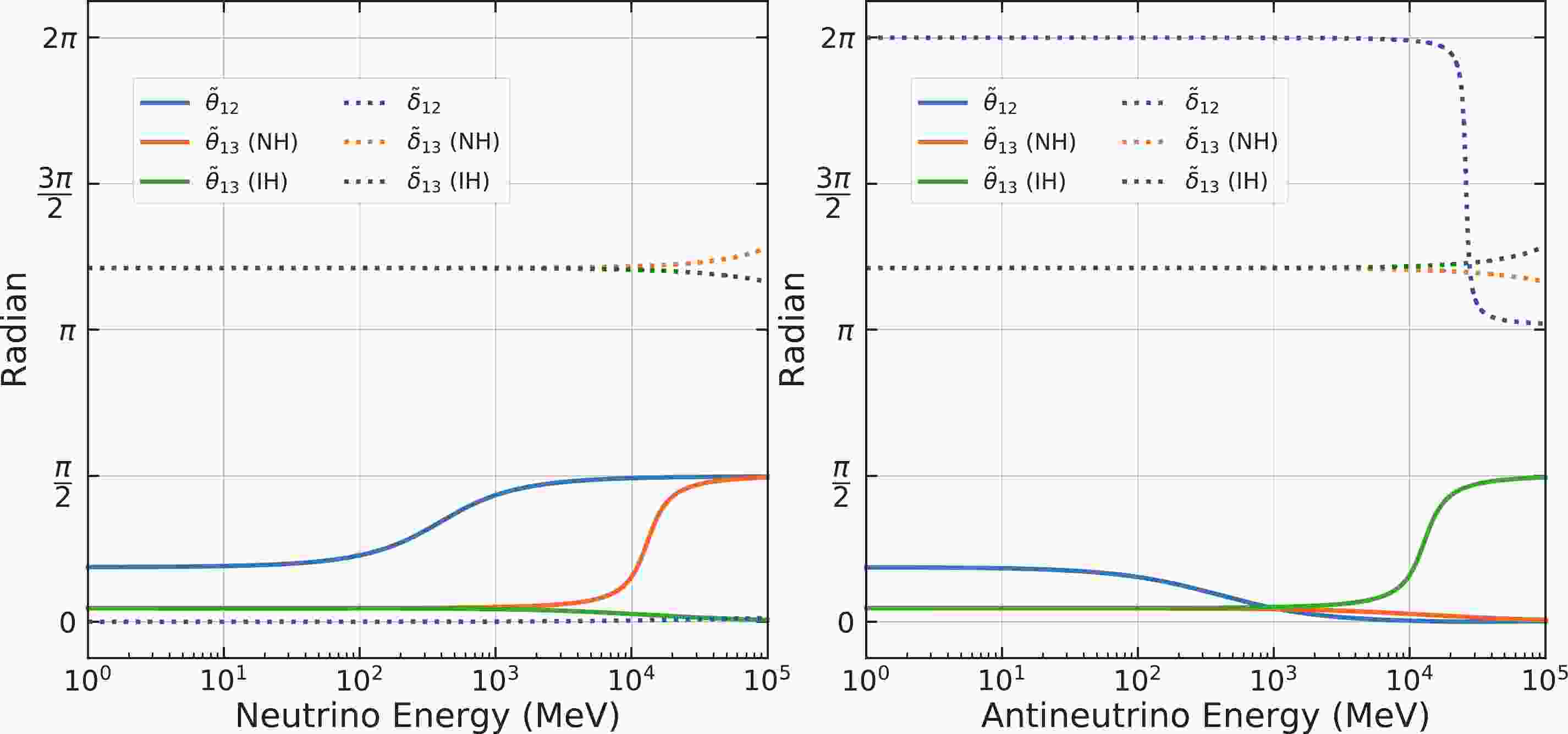
Figure 1. (color online) The values of
$ \widetilde{\theta}_{12} $ ,$ \widetilde{\theta}_{13} $ ,$ \widetilde{\delta}_{12} $ , and$ \widetilde{\delta}_{13} $ with respect to neutrino energy. In this figure, we assume$ \Delta m_{41}^2 = 0.1 $ eV$ ^2 $ ,$ \sin^2\theta_{14} = 0.019 $ ,$ \sin^2\theta_{24} = 0.015 $ ,$ \sin^2\theta_{34} = 0 $ [56],$ \delta_{13} = 218^\circ $ [57] , and$ \delta_{24} = \delta_{34} = 0^\circ $ . The solid and dashed lines represent the effective angles and phases, respectively. The shift of$ \widetilde{\delta}_{12} $ with a factor of$ \pi $ is caused by the transmission of the sign "-" from$ \sin\widetilde{\theta}_{12} $ and$ \cos\widetilde{\theta}_{12} $ , where we set$ \widetilde{\theta}_{12} $ within$ [0,\frac{\pi}{2}] $ , in Eq. (18). In the right-hand plot, as the energy rises,$ \widetilde{\theta}_{12} $ tends to be negative. At that point of time, we shift its negative sign to the phase$ \widetilde{\delta}_{12} $ to ensure that$ \widetilde{\theta}_{12} $ is in the interval$ [0,\frac{\pi}{2}] $ , resulting in a$ \pi $ shift.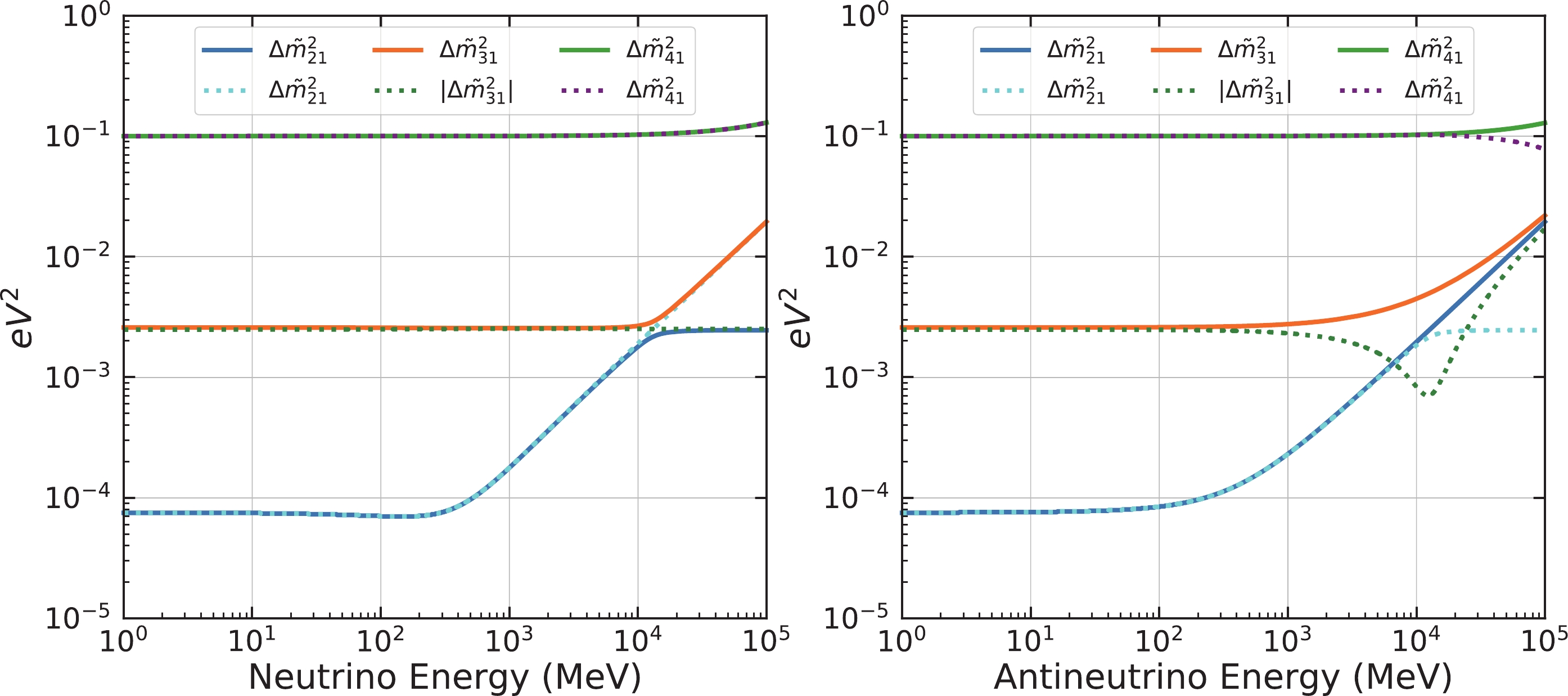
Figure 2. (color online) The values of
$ \Delta\widetilde{m}_{i1}^2(i = 2,3,4) $ with respect to neutrino energy, assuming$ \Delta m_{41}^2 = 0.1 $ eV$ ^2 $ ,$ \sin^2\theta_{14} = 0.019 $ ,$ \sin^2\theta_{24} = 0.015 $ ,$ \sin^2\theta_{34} = 0 $ [56],$ \delta_{13} = 218^\circ $ [57] , and$ \delta_{24} = \delta_{34} = 0^\circ $ . The solid and dashed lines represent NH and IH, respectively. -
The effective matrix
$ \widetilde{U} $ in matter introduces two effective mixing angles$ \widetilde{\theta}_{12} $ and$ \widetilde{\theta}_{13} $ , two effective CP phases$ \widetilde{\delta}_{12} $ and$ \widetilde{\delta}_{13} $ , and effective mass-squared differences$ \Delta \widetilde{m}_{ij}^2 $ , where$ \widetilde{\delta}_{12} $ is an additional parameter introduced from the Jacobi-like method. These effective parameters are clearly energy dependent, as shown in Figs. 1 and 2.In Fig. 1, when
$ E<100 $ MeV,$ \widetilde{\theta}_{12} $ and$ \widetilde{\theta}_{13} $ are very close to the$ \theta_{12} $ and$ \theta_{13} $ values in vacuum. The value of$ \widetilde{\theta}_{12} $ increases (decreases) rapidly up to the maximum$ \frac{\pi}{2} $ (the minimum$ 0 $ ) in the neutrino (antineutrino) energy range from$ 100 $ MeV to$ 10 $ GeV, leading to$ \sin\widetilde{\theta}_{12}\rightarrow 1 $ ($ \sin\widetilde{\theta}_{12}\rightarrow 0 $ ). In contrast,$ \widetilde{\theta}_{13} $ begins to change after$ E>1 $ GeV. It can go up to$ \displaystyle\frac{\pi}{2} $ assuming NH for neutrinos and IH for antineutrinos when$ E>100 $ GeV; it tends to go down to$ 0 $ for the other two combinations. When$ E<1 $ GeV, both the effective CP phases are close to their corresponding vacuum oscillation values ($ \widetilde{\delta}_{12}\rightarrow 0 $ and$ \widetilde{\delta}_{13}\rightarrow\delta_{13} $ ). When the energy increases above$ 1 $ GeV, the influence of the matter effect on$ \widetilde{\delta}_{12} $ and$ \widetilde{\delta}_{13} $ is not negligible.In Fig. 2, the effect of matter also changes the values of the effective neutrino mass-squared differences
$ \Delta \widetilde{m}_{ij}^{2} $ . When$ E<100 $ MeV,$ \Delta \widetilde{m}_{21}^2 $ ,$ \Delta \widetilde{m}_{31}^2 $ , and$ \Delta \widetilde{m}_{41}^2 $ are close to their vacuum values.$ \Delta \widetilde{m}_{21}^2 $ begins to vary when$ E>100 $ MeV, while$ \Delta \widetilde{m}_{31}^2 $ starts to change after$ E>1 $ GeV. In the case of$ \Delta m_{41}^2 = 0.1 $ eV$ ^2 $ with the current sterile neutrino limits,$ \Delta \widetilde{m}_{41}^2 $ is insensitive to the matter effect when$ E<100 $ GeV. As the neutrino energy increases, the matter effect shifts the values of the effective$ \Delta \widetilde{m}_{21}^2 $ more than$ \Delta \widetilde{m}_{31}^2 $ and$ \Delta \widetilde{m}_{41}^2 $ when$ E<100 $ GeV. It should be noted that$ |\Delta\tilde{m}_{31}^2| $ has a dip structure around$ 10 $ GeV for the antineutrino IH case. This feature also shows up in the 3-flavor neutrino case.In general, as shown in Figs. 1 and 2, the matter effect is negligible on both
$ \Delta \widetilde{m}_{21}^2 $ and 1-2 neutrino mixing when$ A_{\rm{CC}} $ ($ A_{\rm{NC}} $ )$ \ll \Delta m_{21}^2 \ll \Delta m_{31}^2 $ (or equivalently$ E\ll100 $ MeV). When the energy increases, it is clear that the 1-2 neutrino mixing submatrix is affected by matter considerably more than the other submatrices. So does$ \Delta \widetilde{m}_{21}^2 $ . However,$ \Delta \widetilde{m}_{31}^2 $ and 1-3 mixing neutrino mixing still hold stable when$ A_{\rm{CC}} $ ($ A_{\rm{NC}} $ )$ \ll \Delta m_{31}^2 $ (or equivalently$ E\ll1 $ GeV). Furthermore, mixing between active and sterile neutrinos has little impact. From a mathematical point of view, in the function of rotation angles yielding$\tan\theta = \displaystyle \frac{2A}{\gamma-\alpha \pm \sqrt{(\gamma-\alpha)^2+4A^2}},$

A is proportional to the values of
$ \theta_{14} $ ,$ \theta_{24} $ , and$ \theta_{34} $ , and$ \gamma-\alpha $ is inversely proportional to$ \Delta m_{41}^2 $ . Hence, the smallness of these mixing angles and large$\Delta m_{41}^2( > 0.1~{\rm eV}^2)$ can effectively suppress the values of the corresponding rotation angles to a negligible level in the submatrices. Therefore, after the rotations on the 1-2 and 2-3 (1-3) submatrices of the neutrino Hamiltonian, the effective Hamiltonian matrix is approximately diagonal.The discussion above pertains to the general feature of our derived oscillation formula. In some particular cases, the oscillation formula can be simplified:
● No CP violations (
$ \delta_{13} = \delta_{24} = \delta_{34} = 0/\pi $ )In such cases, the neutrino mixing matrix is real and it is not necessary to introduce an extra phase
$ \widetilde{\delta}_{12} $ in Eq. (17) for the matrix diagonalization. Thus, this reverts to the original Jacobi method. The neutrino oscillation forms are identical to those in vacuum with$ \widetilde{\theta}_{12} = \theta_{12}+\omega_1 $ ,$ \widetilde{\theta}_{13} = \theta_{13}+{\omega_2} $ , and$ \widetilde{\delta}_{13} = \delta_{13} $ .● No active-sterile neutrino mixing (
$ \theta_{14} = \theta_{24} = \theta_{34} = \delta_{24} = \delta_{34} = 0 $ )The analytical approximations will reduce to 3-flavor neutrino oscillations.
-
All the neutrino oscillation probabilities can be expressed with Eq. (9) based on the effective
$ \widetilde{U} $ and$ \Delta\widetilde{m}_{ij}^2 $ calculated in section 3.2. In this section, we first check the accuracy of these approximations. Then, we highlight the accuracy of this work for two specific long-baseline accelerator neutrino experiments, namely the Tokai to Hyper-Kamiokande (T2HK) and Deep Underground Neutrino Experiment (DUNE). -
The accuracy of our approximations can be quantified with
$ \Delta P_{\nu_\alpha\rightarrow\nu_\beta} $ , which is defined as the numerical difference between the approximations and exact solutions for neutrinos with$ \alpha $ flavor type converting to$ \beta $ type.$ \Delta P_{\nu_\alpha\rightarrow\nu_\beta} = \left|P_{\nu_\alpha\rightarrow\nu_\beta}^{\rm{Exact}}-P_{\nu_\alpha\rightarrow\nu_\beta}^{\rm{Approximate}}\right| \,. $

(27) To check the validity of our approximations, Figure 3 presents the results, as a function of neutrino energy and travel baseline, on four major neutrino oscillation channels, including
$ \nu_{e} \rightarrow \nu_{e} $ ,$ \nu_{\mu} \rightarrow \nu_{\mu} $ disappearance, and$ \nu_{\mu} \rightarrow \nu_{e} $ and$ \nu_{e} \rightarrow \nu_{\mu} $ appearance. The input values for the oscillation parameters are listed in Table 1. Here, we conservatively assume the unknown sterile neutrino associated mixing angles to be as large as$ 20^\circ $ and unknown phases to be maximal, i.e,$ 90^\circ $ .active sterile NH IH $ {\sin^2\theta_{12}} $ 

0.307 $ {\theta_{14}} $ 

$ 20^\circ $ 

$ {\sin^2\theta_{13}} $ 

0.0212 $ {\theta_{24}} $ 

$ 20^\circ $ 

$ {\sin^2\theta_{23}} $ 

0.417 0.421 $ {\theta_{34}} $ 

$ 20^\circ $ 

$ {\Delta m^2_{21}} $ 

$ 7.53\times 10^{-5} $ eV

$ ^2 $ 

$ {\Delta m^2_{41}} $ 

0.1 eV $ ^2 $ 

$ {\Delta m^2_{32}} $ 

$ 2.51 \times 10^{-3} $ eV

$ ^2 $ 

$ -2.56 \times 10^{-3} $ eV

$ ^2 $ 

$ {\delta_{24}} $ 

$ \pi/2 $ 

$ \delta_{13} $ 

$ \pi/2 $ 

$ \delta_{34} $ 

$ \pi/2 $ 

Table 1. Input values for the oscillation parameters. Those associated with active neutrinos except
$ \delta_{13} $ are derived from recent results [57]. The sterile neutrino values are conservatively using relatively large values.
Figure 3. (color online) The accuracies of the approximations in different oscillation channels with
$ \Delta P_{\nu_\alpha\rightarrow\nu_\beta} $ .As shown in Fig. 3, when the neutrino energy is below
$ 20 $ GeV, the accuracy is better than$ 10^{-3} $ and$ 10^{-4} $ for the neutrino disappearance and appearance channels, respectively. The accuracy will improve by one or two orders when the neutrino energy is smaller. The numerical accuracy of our approximations was relatively good for most of the long baseline neutrino oscillation experiments, as the difference is approximately one order smaller than the oscillation probabilities. The inaccuracy of our approach can be mainly attributed to the limited rotation iterations that were applied. One approach to further improve the accuracy is to apply some corrections based on the perturbative method after matrix rotation, as shown in Ref. [58]. Naturally, this will increase the complexity of the analytical expression. Our current approximations achieve a good balance between the numerical accuracy and simplicity of the approximation expressions. It should be noted that the exact accuracy of the approximations depends on the exact neutrino mixing parameter inputs. Once the sterile neutrino mixing angles are smaller than$ 20^{\circ} $ and$ \Delta m^{2}_{41} $ is larger than$ 0.1 $ eV2, the accuracy of our expressions will further impove compared with the current evaluation. -
As shown in Eqs. (7) and (8), the matter effect is proportional to the neutrino beam energy and its propagation distance. Hence, the matter effect can significantly modify the neutrino oscillation features for long-baseline neutrino oscillation experiments, such as T2HK and DUNE. These experiments have relatively high energy beams at
$ \sim $ GeV and baselines of hundreds and thousands of kilometers. Here, we use them as examples to demonstrate 3+1-neutrino oscillation and check the accuracy of our approximations.DUNE is a next generation on-axis long-baseline accelerator neutrino experiment. It proposes the use of Liquid Argon (LAr) detectors located deep underground,
$ 1300 $ km away from the beam source. Its main physics goals are to solve three challenging issues in the neutrino sector, namely neutrino mass hierarchy, CP asymmetry, and the octant of$ \theta_{23} $ . It can search for electron and tau neutrino (anti-neutrino) appearance and muon neutrino (antineutrino) disappearance channels from both the neutrino and antineutrino beam modes.T2HK is a proposed long-baseline experiment that has the primary objective of measuring CP asymmetry. The far detector is
$ 295 $ km away and$ 2.5^\circ $ off-axis from the J-PARC beam in Japan, when using the water Cherenkov detector.Considering the existence of sterile neutrinos with a relatively large mass-squared difference
$ \Delta m_{41}^2 = 0.1 $ eV$ ^2 $ , the high-frequency oscillation feature is clearly shown in the muon neutrino disappearance and electron neutrino appearance modes in Fig. 4. Given the matter effect and CP-violation phases, the electron neutrino and antineutrino appearance probabilities$ P_{\nu_\mu\rightarrow\nu_e} $ and$ P_{\bar{\nu}_\mu\rightarrow\bar{\nu}_e} $ are very different. Compared with the numerical calculations, the accuracy of the analytical approximations can reach$ 10^{-5} $ in the case of Table 1 for neutrinos and antineutrinos, respectively, for the appearance mode. For the disappearance mode, the accuracies of$ P_{\nu_\mu\rightarrow\nu_\mu} $ and$ P_{\bar{\nu}_\mu\rightarrow\bar{\nu}_\mu} $ can reach$ 10^{-4} $ in the case of Table 1.
Figure 4. (color online) The left-hand plots correspond to the appearance channels, and the right-hand plots show the disappearance channels in the case of NH. The appendant plots show the accuracies of their corresponding channels.
In Fig. 5, we compare the accuracy of this work with that of two previous studies for the T2HK and DUNE experiments. Our work clearly shows about an order of better accuracy compared with the other two [50, 60], especially for the DUNE experiment. To achieve a higher accuracy of the approximation, we can continue introducing a perturbation correction later on the effective neutrino mixing and mass-squared differences, as adopted in [58]. However, given that the accuracy of this work is already substantially good for current and near-future experiments, we do not believe this is necessary.

Figure 5. (color online) Comparison of
$ P_{\bar{\nu}_\mu\rightarrow\bar{\nu}_e} $ between DUNE and T2HK in the case of NH with the values listed in Table 1 except the phases. We adopt$ \delta_{13} = 90^\circ $ and$ \delta_{14} = 90^\circ $ according to the convention used by N. Klop et al. [50]. Similar to the examples shown in their paper, we combine this with a Neutral Current NSI solution [59] to produce the oscillation probability. -
The search for light sterile neutrinos is an area of great interest in the neutrino field. Many long baseline neutrino experiments continue to actively search for light sterile neutrinos in various mass regions. Both CC and NC induced matter effects are quite important for those experiments. The analytical approximations of neutrino oscillation are preferred in experimental neutrino research because they save considerable time and are helpful for understanding the neutrino oscillation features.
In this manuscript, we introduced a Jacobi-like method to derive simplified analytical expressions with good accuracy for neutrino oscillation in matter. Compact expressions of the effective mixing matrix
$ \widetilde{U} $ and effective mass-squared differences$ \Delta\widetilde{m}_{ij}^2(i,j = 1,2,3,4) $ were presented. The accuracy of this work is sufficient for a majority of long baseline neutrino experiments.In addition, the Jacobi-like method is a general method for diagonalizing complex Hermitian matrices. It can also be extended to other physics topics, such as 3 (active) + N (sterile)-neutrino mixing and neutrino non-standard interactions.
We would like to extend our thanks to Yu-Feng Li for the valuable discussions and to Neill Raper for helping with the editing of this manuscript.
-
In the 3 + 1 framework, neutrino mixing can be written as a
$ 4\times 4 $ matrix (5). 6 rotation angles with 3 Dirac phases③ are found in this matrix. All the elements of the mixing matrix are listed in Table A1. Indeed, if we set the angles and Dirac phases introduced by sterile neutrinos to 0, the$ 4\times4 $ matrix will reduce to 3-flavor neutrino mixing.$\alpha$ 

$U_{\alpha i}$ 

- e $U_{e1}$ 

$c_{12}c_{13}c_{14}$ 

$U_{e2}$ 

$c_{13}c_{14}s_{12}$ 

$U_{e3}$ 

$c_{14}s_{13}{\rm e}^{-{\rm i}\delta_{13}}$ 

$U_{e4}$ 

$s_{14}$ 

$\mu$ 

$U_{\mu1}$ 

$-s_{12}c_{23}c_{24}-c_{12}(s_{13}c_{24}s_{23}{\rm e}^{{\rm i}\delta_{13} }+c_{13}s_{14}s_{24}{\rm e}^{-{\rm i}\delta_{24} })$ 

$U_{\mu2}$ 

$c_{12}c_{23}c_{24}-s_{12}(s_{13}c_{24}s_{23}{\rm e}^{{\rm i}\delta_{13} }+c_{13}s_{14}s_{24}{\rm e}^{-{\rm i}\delta_{24} })$ 

$U_{\mu3}$ 

$c_{13}c_{24}s_{23}-s_{13}s_{14}s_{24}{\rm e}^{-{\rm i}\delta_{13}}{\rm e}^{-{\rm i}\delta_{24}}$ 

$U_{\mu4}$ 

$c_{14}s_{24}{\rm e}^{-{\rm i}\delta_{24}}$ 

$\tau$ 

$U_{\tau1}$ 

$\begin{aligned} c_{12}[s_{13}(s_{23}s_{24}s_{34}{\rm e}^{{\rm i}\delta_{24}}{\rm e}^{-{\rm i}\delta_{34}}-c_{23}c_{34}){\rm e}^{{\rm i}\delta_{13}}-c_{13}c_{24}s_{14}s_{34}{\rm e}^{-{\rm i}\delta_{34}}] +s_{12}(c_{34}s_{23}+c_{23}s_{24}s_{34}{\rm e}^{{\rm i}\delta_{24}}{\rm e}^{-{\rm i}\delta_{34}}) \end{aligned}$ 

$U_{\tau2}$ 

$\begin{aligned} s_{12}[s_{13} (s_{23}s_{24}s_{34}{\rm e}^{{\rm i}\delta_{24}}{\rm e}^{-{\rm i}\delta_{34}}-c_{23}c_{34}){\rm e}^{{\rm i}\delta_{13}} -c_{13}c_{24}s_{14}s_{34}{\rm e}^{-{\rm i}\delta_{34}}] -c_{12}(c_{34}s_{23}+c_{23}s_{24}s_{34}{\rm e}^{-{\rm i}\delta_{34}} )\end{aligned}$ 

$U_{\tau3}$ 

$c_{13}(c_{23}c_{34}-s_{23}s_{24}s_{34}{\rm e}^{{\rm i}\delta_{24}}{\rm e}^{-{\rm i}\delta_{34}})-s_{13}c_{24}s_{14}s_{34}{\rm e}^{-{\rm i}\delta_{13}}{\rm e}^{-{\rm i}\delta_{34}}$ 

$U_{\tau4}$ 

$c_{14}c_{24}s_{34}{\rm e}^{-{\rm i}\delta_{34}}$ 

s $U_{s1}$ 

$ c_{12}[s_{13}(c_{34}s_{23}s_{24}e^{i\delta_{24}}+c_{23}s_{34}{\rm e}^{{\rm i}\delta_{34}}){\rm e}^{{\rm i}\delta_{13}}-c_{13}c_{24}c_{34}s_{14}] + s_{12}(c_{23}c_{34}s_{24}{\rm e}^{{\rm i}\delta_{24}}-s_{23}s_{34}{\rm e}^{{\rm i}\delta_{34}}) $ 

$U_{s2}$ 

$ s_{12}[s_{13} (c_{34}s_{23}s_{24}{\rm e}^{{\rm i}\delta_{24}}+c_{23}s_{34} {\rm e}^{{\rm i}\delta_{34}}){\rm e}^{{\rm i}\delta_{13}}-c_{13}c_{24}c_{34}s_{14}] +c_{12}(s_{23}s_{34}{\rm e}^{{\rm i}\delta_{34}}-c_{23}c_{34}s_{24}{\rm e}^{{\rm i}\delta_{24}}) $ 

$U_{s3}$ 

$-c_{13}(c_{34}s_{23}s_{24}{\rm e}^{{\rm i}\delta_{24}}+c_{23}s_{34}{\rm e}^{{\rm i}\delta_{34}})-c_{24}c_{34}s_{14}{\rm e}^{-{\rm i}\delta_{13}}$ 

$U_{s4}$ 

$c_{14}c_{24}c_{34}$ 

Table A1. Elements of the 4-flavor mixing matrix.
-
The matter effect for the 3+1 framework is more difficult to calculate than for the 3 neutrino framework because additional parameters are involved in the neutrino Hamiltonian, which is a
$ 4\times4 $ complex Hermitian matrix and difficult to diagonalize. In this work, we adopt a rotation technique known as the Jacobi-like method to solve the diagonalization for complex Hermitian matrices. In the following subsections, we provide all the technical details for the neutrino and antineutrino cases separately. -
In this subsection, we show the diagonalization of the effective Hamiltonian with the matter effect and simplify the expressions of the effective mixing and mass-squared differences for the neutrino case.
-
In the case of neutrinos, we find that the absolute values of the elements
$ H_{12} $ and$ H_{21} $ in Eq. (10) are the relatively largest off-diagonal values because of the smallness of$ \Delta m_{21}^2 $ . Hence, we should diagonalize the 1-2 submatrix first.First rotation: The rotation matrix can be written as
$\tag{B1} \begin{split}& R^1 = R_{12}({\omega_1},\phi_1)\equiv \begin{bmatrix} c_{{\omega_1}}&s_{{\omega_1}}{\rm e}^{-{\rm i}\phi_1}&0&0\\ -s_{{\omega_1}}{\rm e}^{{\rm i}\phi_1}&c_{{\omega_1}}&0&0\\ 0&0&1&0\\ 0&0&0&1 \end{bmatrix}\,. \\& (c_{{\omega_1}} = \cos{\omega_1} \,,s_{{\omega_1}} = \sin{\omega_1}) \end{split} $

(B1) We employ the Jacobi-like method to derive
$ {\omega_1} $ yielding$\tag{B2} \begin{split}& \tan{\omega_1} = \frac{2A_{{\omega_1}}}{(H_{22}-H_{11})+ \sqrt{(H_{22}-H_{11})^2+4A_{{\omega_1}}^2}} \,,\\& (0< {\omega_1} <\frac{\pi}{2}-{\theta}_{12})\end{split} $

(B2) with
$ A_{{\omega_1}} = |H_{12}| $ and$ \phi_1 = {\rm{Arg}}(\mathrm{sign}(A_{\omega_1})H_{12}^{*}) $ . Here$ A_{{\omega_1}} $ is the amplitude of$ H_{12} $ . After rotation by$ R_{12}({\omega_1},\phi_1) $ , we rewrite the Hamiltonian in the new representation as$\tag{B3} H^\prime = R_{12}^\dagger({\omega_1},\phi_1) H R_{12}({\omega_1},\phi_1) = \frac{1}{2E} \begin{bmatrix} \lambda_{-} &0 &H_{13}^{\prime} & H_{14}^{\prime } \\ 0 & \lambda_{+} & H_{23}^{\prime } & H_{24}^{\prime} \\ H_{31}^{\prime } & H_{32}^{\prime } & H_{33} & H_{34} \\ H_{41}^{\prime } & H_{42}^{\prime } & H_{43}& H_{44} \end{bmatrix}\,, $

(B3) with the eigenvalues of the 1-2 submatrix
$\tag{B4} \begin{split} & \lambda_- = \frac{H_{11}+H_{22}\tan^2{\omega_1}-2A_{\omega_1}\tan{\omega_1}} {1+\tan^2{\omega_1}} \,, \\ & \lambda_+ = \frac{H_{11}\tan^2{\omega_1}+H_{22}+2A_{\omega_1}\tan{\omega_1}} {1+\tan^2{\omega_1}} \,.\end{split} $

(B4) The corresponding off-diagonal terms in
$ H^\prime $ are$\quad\quad\quad\quad\quad\tag{B5} H_{13}^\prime = H_{31}^{\prime *} = c_{\omega_1}H_{13}-s_{\omega_1} H_{23}{\rm e}^{-{\rm i}\phi_1} \,, $

(B5) $\quad\quad\quad\quad\quad\tag{B6} H_{23}^\prime = H_{32}^{\prime *} = c_{\omega_1}H_{23} + s_{\omega_1} H_{13}{\rm e}^{{\rm i}\phi_1} \,, $

(B6) $\quad\quad\quad\quad\quad \tag{B7} H_{14}^\prime = H_{41}^{\prime *} = c_{\omega_1}H_{14} - s_{\omega_1} H_{24}{\rm e}^{-{\rm i}\phi_1} \,, $

(B7) $\quad\quad\quad\quad\quad \tag{B8} H_{24}^\prime = H_{42}^{\prime *} = c_{\omega_1}H_{24} + s_{\omega_1} H_{14}{\rm e}^{{\rm i}\phi_1} \,. $

(B8) After the first rotation, we can diagonalize the 2-3 submatrix later because it has a relatively large off-diagonal element and is useful for simplifying the effective matrix U using Eq. (B22).
Second rotation: The second rotation matrix yields
$ \tag{B9} \begin{split} & R^2 = R_{23}({\omega_2},{\phi_2}) \equiv \begin{bmatrix} 1&0&0&0\\ 0&c_{{\omega_2}}&s_{{\omega_2}}{\rm e}^{-{\rm i}{\phi_2}}&0\\ 0&-s_{{\omega_2}}{\rm e}^{{\rm i}{\phi_2}}&c_{{\omega_2}}&0\\ 0&0&0&1 \end{bmatrix}\,.\\ & (c_{{\omega_2}} = \cos{\omega_2},s_{{\omega_2}} = \sin{\omega_2})\end{split} $

(B9) The diagonal angle
$ {\omega_2} $ is compatible with$\tag{B10} \tan{\omega_2} = \frac{2A_{\omega_2}}{(H_{33}-\lambda_+)\pm \sqrt{(H_{33}-\lambda_+)^2+4A_{\omega_2}^2}} \,, $

(B10) where the upper sign is for NH
$ (0 < {\omega_2} < \frac{\pi}{2}-\theta_{13}) $ , and the lower sign is for IH$ ( 0 > {\omega_2} > -\theta_{13}) $ .$ A_{{\omega_2}} $ is the amplitude of$ H_{23} $ in Eq. (B3) yielding$ A_{{\omega_2}} = |H_{23}^\prime| $ . The additional complex factor is given by$ \phi_2 = {\rm{Arg}}(\mathrm{sign}(A_{\omega_2})H_{23}^{\prime*}) $ . After two rotations, we obtain$\tag{B11} \begin{split}\!\!\! H^{\prime\prime} & = R_{23}^\dagger({\omega_2},{\phi_2}) H^{\prime} R_{23}({\omega_2},{\phi_2}) = \frac{1}{2E} \begin{bmatrix} \lambda_{-}& H_{12}^{\prime\prime}&H_{13}^{\prime\prime}&H_{14}^{\prime}\\ H_{21}^{\prime\prime}&\lambda_-^{\prime}&0&H_{24}^{\prime\prime}\\ H_{31}^{\prime\prime}&0&\lambda_{+}^{\prime}&H_{34}^{\prime\prime}\\ H_{41}^{\prime}&H_{42}^{\prime\prime}&H_{43}^{\prime\prime}&H_{44} \end{bmatrix} \,,\end{split} $

(B11) where the diagonal terms
$ \lambda_-^\prime $ and$ \lambda_+^\prime $ obey$ \tag{B12} \begin{split} & \lambda_-^\prime = \frac{\lambda_+ +H_{33}\tan^2{\omega_2}-2A_{\omega_2}\tan{\omega_2}} {1+\tan^2{\omega_2}} \,,\\ & \lambda_+^\prime = \frac{\lambda_+\tan^2{\omega_2}+H_{33}+2A_{\omega_2}\tan{\omega_2}} {1+\tan^2{\omega_2}} \,.\end{split} $

(B12) The corresponding off-diagonal elements obey
$\tag{B13} H^{\prime\prime}_{12} = H^{\prime\prime*}_{21} = - s_{\omega 2} H_{13}^\prime {\rm e}^{{\rm i}\phi_2} \,, $

(B13) $ \tag{B14} H^{\prime\prime}_{13} = H^{\prime\prime*}_{31} = c_{\omega 2} H_{13}^\prime \,, $

(B14) $\tag{B15} H^{\prime\prime}_{24} = H^{\prime\prime*}_{42} = c_{\omega 2} H_{24}^\prime - s_{\omega 2} H_{34} {\rm e}^{-{\rm i}\phi_2} \,, $

(B15) $\tag{B16} H^{\prime\prime}_{34} = H^{\prime\prime*}_{43} = c_{\omega 2} H_{34} + s_{\omega 2} H_{24}^\prime {\rm e}^{{\rm i}\phi_2} \,. $

(B16) After two continuous rotations, the matrix is approximately diagonalized. We can evaluate the matrix diagonalization using the ratio defined as
$ \tag{B17} R_{ij}\equiv\left|\frac{H^{\prime\prime}_{ij}}{H^{\prime\prime}_{jj}-H^{\prime\prime}_{ii}}\right| \,(i<j), $

(B17) which compares the relative size of the off-diagonal elements in
$ H^{\prime\prime} $ with the difference between the two corresponding diagonal terms. Figure B1 shows the ratios for various submatrices with respect to the neutrino energy. All of these are considerably smaller than$ 0.1 $ , which means that the corresponding rotation angles on the$ i-j $ submatrix of$ H^{\prime\prime} $ will be considerably smaller than$ 5^\circ $ based on section 3.1. Thus, the$ H^{\prime\prime} $ matrix can be treated as an approximately diagonalized matrix in our application range.
Figure B1. (color online) The values of the off-diagonal elements in
$ H^{\prime\prime} $ . The solid and dashed lines correspond to NH and IH, respectively. The input oscillation parameters are listed in Table 1.After diagonalization, the effective neutrino mixing matrix and mass-squared differences are given by
$ \begin{split} \widetilde{U} & \approx UR_{12}(\omega_1,\phi_1)R_{23}({\omega_2},{\phi_2}) \\ & = \underbrace{R_{34}R_{24}R_{14}R_{23}R_{13}R_{12}}_{U} R_{12}(\omega_1,\phi_1)R_{23}({\omega_2},{\phi_2}) \,, \end{split} \tag{B18a}$

(B18a) $ \tag{B18b} \Delta \widetilde{m}_{21}^2\approx\lambda_{-}^{\prime}-\lambda_- \,,\;\; \Delta \widetilde{m}_{31}^2\approx\lambda_{+}^{\prime}-\lambda_- \,,\;\; \Delta \widetilde{m}_{41}^2\approx H_{44}-\lambda_- \,. $

(B18b) If
$ \delta_{13} = \delta_{24} = \delta_{34} = 0 $ ,$ \phi_1 $ and$ {\phi_2} $ will be 0. To establish the beauty of the mathematical form (it is convenient for$ \widetilde{U} $ to completely have the same form with U) and a good understanding of the matter effect on the oscillation parameters, we continue to simplify the effective mixing matrix$ \widetilde{U} $ below. -
First, we can observe that there are two 1-2 submatrix rotations
$ R_{12}(\theta_{12},0) $ and$ R_{12}(\omega_1,\phi_1) $ next to each other in Eq. (B18b). Therefore, we combine them into one submatrix. The corresponding processes are given by$ \begin{split} &R_{12}(\theta_{12},0)R_{12}(\omega_1,\phi_1)\\ = & \begin{bmatrix} c_{12}&s_{12}&0&0\\ -s_{12}&c_{12}&0&0\\ 0&0&1&0\\ 0&0&0&1 \end{bmatrix} \begin{bmatrix} c_{\omega_1}&s_{\omega_1}{\rm e}^{-{\rm i}\phi_1}&0&0\\ -s_{\omega_1}{\rm e}^{{\rm i}\phi_1}&c_{\omega_1}&0&0\\ 0&0&1&0\\ 0&0&0&1 \end{bmatrix} \\ = & \begin{bmatrix} \widetilde{c}_{12}&\widetilde{s}_{12}{\rm e}^{-{\rm i}\widetilde{\delta}_{12}}&0&0\\ -\widetilde{s}_{12}{\rm e}^{{\rm i}\widetilde{\delta}_{12}}&\widetilde{s}_{12}&0&0\\ 0&0&1&0\\ 0&0&0&1 \end{bmatrix} \begin{bmatrix} {\rm e}^{{\rm i}\Theta_{12}}&0&0&0\\ 0&{\rm e}^{-{\rm i}\Theta_{12}}&0&0\\ 0&0&1&0\\ 0&0&0&1 \end{bmatrix} \\ = & R_{12}(\widetilde{\theta}_{12},\widetilde{\delta}_{12})D_{12}({\rm e}^{{\rm i}\Theta_{12}},{\rm e}^{-{\rm i}\Theta_{12}},1,1) = \widetilde{R}_{12}. \end{split} \tag{B19} $

(B19) Then, we obtain
$ \widetilde{U}\approx R_{34}R_{24}R_{14}R_{23}R_{13}\widetilde{R}_{12}R_{23}({\omega_2},{\phi_2}) \,. \tag{B20}$

(B20) We can observe that there is a new
$ \widetilde{R}_{12} $ consisting of a rotation matrix with$ \widetilde{\theta}_{12} $ and$ \widetilde{\delta}_{12} $ and one diagonal unitary matrix with phase$ \Theta_{12} $ . These new items yield$ \quad\quad\quad\quad\begin{split}& \widetilde{s}_{12} = \sin\widetilde{\theta}_{12} = \frac{|c_{12}\tan\omega_1 {\rm e}^{{\rm i}\phi_1}+s_{12}|}{\sqrt{1+\tan^2\omega_1}} \,, \\ \quad\quad\quad\quad& \widetilde{c}_{12} = \cos\widetilde{\theta}_{12} = \frac{|c_{12}-s_{12}\tan\omega_1 {\rm e}^{{\rm i}\phi_1}|}{\sqrt{1+\tan^2\omega_1}} \,, \end{split} \tag{B21a} $

(B21a) $ {\rm e}^{{\rm i}\widetilde{\delta}_{12}} = \frac{(c_{12}\tan\omega_1 {\rm e}^{{\rm i}\phi_1}+s_{12})(c_{12}-s_{12}\tan \omega_1 {\rm e}^{-{\rm i}\phi_1})} {\cos \widetilde{\theta}_{12} \sin \widetilde{\theta}_{12} (1+\tan^2 \omega_1 )} \,, \tag{B21b} $

(B21b) $ {\rm e}^{{\rm i}\Theta_{12}} = \frac{c_{12}-s_{12}\tan\omega_1 {\rm e}^{\phi_1}} {\cos\widetilde{\theta}_{12}\sqrt{1+\tan^2\omega_1}} \,. \tag{B21c} $

(B21c) Here, we set the same limit on
$ \widetilde{\theta}_{12} $ in$ [0,\frac{\pi}{2}] $ with$ \theta_{12} $ .To maintain a similar oscillation expression to the extent possible as its form in vacuum, we replace
$ \widetilde{R}_{12} R_{23}(\omega_2,\phi_2) $ with$ \widetilde{R}_{12} R_{23}({\omega_2},{\phi_2})\approx R_{13}({\omega_2},{\phi_2})\widetilde{R}_{12} \,, \tag{B22}$

(B22) where
$ \widetilde{R}_{12}R_{23}(\omega_2,\phi_2) $ can be expressed as$ \widetilde{R}_{12}R_{23}(\omega_2,\phi_2) = \begin{bmatrix} \widetilde{c}_{12} {\rm e}^{{\rm i}\Theta_{12}} & c_{\omega_2} \widetilde{s}_{12}{\rm e}^{-{\rm i}(\widetilde{\delta}_{12}+\Theta_{12})} & \widetilde{s}_{12}s_{\omega_2}{\rm e}^{-{\rm i}(\widetilde{\delta}_{12}+\Theta_{12}+\phi_2)} & 0 \\ -\widetilde{s}_{12}{\rm e}^{{\rm i}(\widetilde{\delta}_{12}+\Theta_{12})} & \widetilde{c}_{12}c_{\omega_2}{\rm e}^{-{\rm i}\Theta_{12}} & \widetilde{c}_{12}s_{\omega_2} {\rm e}^{-{\rm i}(\Theta_{12}+\phi_2)} & 0 \\ 0 & -s_{\omega_2}{\rm e}^{{\rm i}\phi_2} & c_{\omega_2} & 0 \\ 0 & 0 & 0 & 1 \end{bmatrix} \,, \tag{B23}$

(B23) and
$ R_{13}(\omega_2,\phi_2)\widetilde{R}_{12} $ yields$ R_{13}(\omega_2,\phi_2)\widetilde{R}_{12} = \begin{bmatrix} \widetilde{c}_{12}c_{\omega_2}{\rm e}^{{\rm i}\Theta_{12}} & c_{\omega_2}\widetilde{s}_{12} {\rm e}^{-{\rm i}(\widetilde{\delta}_{12}+\Theta_{12})} & s_{\omega_2}{\rm e}^{-{\rm i}\phi_2} & 0 \\ -\widetilde{s}_{12}{\rm e}^{{\rm i}(\widetilde{\delta}_{12}+\Theta_{12})} & \widetilde{c}_{12}{\rm e}^{-{\rm i}\Theta_{12}} & 0 & 0 \\ -\widetilde{c}_{12}s_{\omega_2} {\rm e}^{{\rm i}(\Theta_{12}+\phi_2)} & -\widetilde{s}_{12}s_{\omega_2}{\rm e}^{{\rm i}(\phi_2-\Theta_{12}-\widetilde{\delta}_{12})} & c_{\omega_2} & 0 \\ 0 & 0 & 0 & 1 \end{bmatrix}\,. \tag{B24}$

(B24) To check the validity of Eq. (B22), we compare all the corresponding elements between
$ \widetilde{R}_{12}R_{23}(\omega_2,\phi_2) $ and$ R_{13}(\omega_2,\phi_2)\widetilde{R}_{12} $ . As shown in Fig. B2, the differences between those two matrices are quite small in our application range.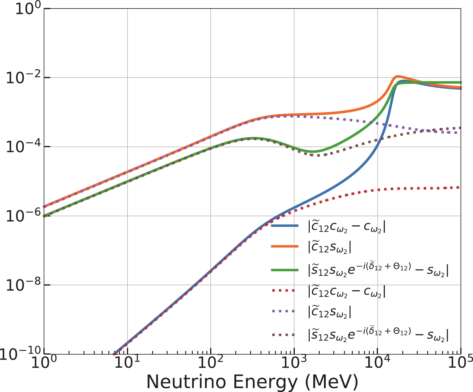
Figure B2. (color online) Differences between
$\widetilde{R}_{12}R_{23}(\omega_2, $ $ \phi_2) $ and$ R_{13}(\omega_2,\phi_2)\widetilde{R}_{12} $ . The solid and dashed lines correspond to NH and IH, respectively. The input oscillation parameters are listed in Table 1.Subsequently, we obtain
$\begin{split} \widetilde{U} & \approx R_{34}R_{24}R_{14}R_{23}R_{13}\widetilde{R}_{12}R_{23}({\omega_2},{\phi_2}) \\ & = R_{34}R_{24}R_{14}R_{23}R_{13}R_{13}({\omega_2},{\phi_2})\widetilde{R}_{12} \,, \end{split}\tag{B25} $

(B25) where
$ \begin{split} &R_{13}(\theta_{13},0)R_{13}({\omega_2},{\phi_2})\\ = & \begin{bmatrix} c_{13}&0&s_{13}{\rm e}^{-{\rm i}\delta_{13}}&0\\ 0&1&0&0\\ -s_{13}{\rm e}^{{\rm i}\delta_{13}}&0&c_{13}&0\\ 0&0&0&1 \end{bmatrix} \begin{bmatrix} c_{{\omega_2}}&0&s_{{\omega_2}}{\rm e}^{-{\rm i}{\phi_2}}&0\\ 0&1&0&0\\ -s_{{\omega_2}}{\rm e}^{{\rm i}{\phi_2}}&0&c_{{\omega_2}}&0\\ 0&0&0&1 \end{bmatrix} \\ = & \begin{bmatrix} \widetilde{c}_{13}&0&\widetilde{s}_{13}{\rm e}^{-{\rm i}\widetilde{\delta}_{13}}&0\\ 0&1&0&0\\ -\widetilde{s}_{13}{\rm e}^{{\rm i}\widetilde{\delta}_{13}}&0&\widetilde{c}_{13}&0\\ 0&0&0&1 \end{bmatrix} \begin{bmatrix} {\rm e}^{{\rm i}\Theta_{13}}&0&0&0\\ 0&1&0&0\\ 0&0&{\rm e}^{-{\rm i}\Theta_{13}}&0\\ 0&0&0&1 \end{bmatrix} \\ = & R_{13}(\widetilde{\theta}_{13},\widetilde{\delta}_{13}) D_{13}({\rm e}^{{\rm i}\Theta_{13}},1,{\rm e}^{-{\rm i}\Theta_{13}},1). \end{split} \tag{B26} $

(B26) The items above can be written as
$ \begin{split}& \widetilde{s}_{13} = \sin \widetilde{\theta}_{13} = \frac{|c_{13}\tan {\omega_2} {\rm e}^{{\rm i}{\phi_2}}+s_{13}{\rm e}^{{\rm i}\delta_{13}}|} {\sqrt{1+\tan^2 {\omega_2} }} \,, \\ & \widetilde{c}_{13} = \cos \widetilde{\theta}_{13} = \frac{|c_{13}-s_{13}\tan {\omega_2} {\rm e}^{{\rm i}(\delta_{13}-{\phi_2})}|} {\sqrt{1+\tan^2 {\omega_2} }} \,, \end{split} \tag{B27a}$

(B27a) $ {\rm e}^{{\rm i}\widetilde{\delta}_{13}} = \frac{(c_{13}\tan {\omega_2} {\rm e}^{{\rm i}{\phi_2}} +s_{13}{\rm e}^{{\rm i}\delta_{13}})(c_{13}-s_{13}\tan {\omega_2} {\rm e}^{{\rm i}(\delta_{13}-{\phi_2})})} {\cos \widetilde{\theta}_{13} \sin \widetilde{\theta}_{13} (1+\tan^2 {\omega_2} )} \,, \tag{B27b} $

(B27b) $ {\rm e}^{{\rm i}\Theta_{13}} = \frac{c_{13}-s_{13}\tan{\omega_2}{\rm e}^{-{\rm i}(\delta_{13}-{\phi_2})}} {\cos\widetilde{\theta}_{13}\sqrt{1+\tan^2{\omega_2}}} \,. \tag{B27c} $

(B27c) Equally, we set the limit on
$ \widetilde{\theta}_{13} $ within$ [0,\frac{\pi}{2}] $ . We find$ \widetilde{U}\approx R_{34}R_{24}R_{14}R_{23} R_{13}(\widetilde{\theta}_{13},\widetilde{\delta}_{13})D_{13}\widetilde{R}_{12} \,. \tag{B28}$

(B28) For the same purpose of simplification, we replace
$ D_{13} \widetilde{R}_{12} $ by$ D_{13}({\rm e}^{{\rm i}\Theta_{13}},1,{\rm e}^{-{\rm i}\Theta_{13}},1) \widetilde{R}_{12} \approx \widetilde{R}_{12} D_{23}(1,{\rm e}^{{\rm i}\Theta_{13}},{\rm e}^{-{\rm i}\Theta_{13}},1) \,, \tag{B29}$

(B29) where
$ \begin{split}& D_{13}({\rm e}^{{\rm i}\Theta_{13}},1,{\rm e}^{-{\rm i}\Theta_{13}},1) \widetilde{R}_{12} = \\& \begin{bmatrix} \widetilde{c}_{12}{\rm e}^{{\rm i}(\Theta_{12}+\Theta_{13})} & \widetilde{s}_{12}{\rm e}^{{\rm i}(\Theta_{13}-\widetilde{\delta}_{12}-\Theta_{12})} & 0 & 0 \\ -\widetilde{s}_{12} {\rm e}^{{\rm i}(\widetilde{\delta}_{12}+\Theta_{12})} & \widetilde{c}_{12}{\rm e}^{-{\rm i}\Theta_{12}} & 0 & 0 \\ 0 & 0 & {\rm e}^{-{\rm i}\Theta_{13}} & 0 \\ 0 & 0 & 0 & 1 \end{bmatrix} \end{split} \tag{B30} $

(B30) and
$ \begin{split} & \widetilde{R}_{12} D_{23}(1,{\rm e}^{{\rm i}\Theta_{13}},{\rm e}^{-{\rm i}\Theta_{13}},1) = \\ & \begin{bmatrix} \widetilde{c}_{12} {\rm e}^{{\rm i}\Theta_{12}} & \widetilde{s}_{12} {\rm e}^{{\rm i}(\Theta_{13}-\widetilde{\delta}_{12}-\Theta_{12})} & 0 & 0 \\ -\widetilde{s}_{12}{\rm e}^{{\rm i}(\widetilde{\delta}_{12}+\Theta_{12})} & \widetilde{c}_{12} {\rm e}^{{\rm i}(\Theta_{13}-\Theta_{12})} & 0 & 0 \\ 0 & 0 & {\rm e}^{-\Theta_{13}} & 0 \\ 0 & 0 & 0 & 1 \end{bmatrix}\,. \end{split} \tag{B31} $

(B31) Figure B3 quantifies the difference between
$D_{13}({\rm e}^{{\rm i}\Theta_{13}}, 1,{\rm e}^{-{\rm i}\Theta_{13}},1)\widetilde{R}_{12}$ and$\widetilde{R}_{12} D_{23}(1,{\rm e}^{{\rm i}\Theta_{13}},{\rm e}^{-{\rm i}\Theta_{13}},1)$ . Such an operation is permissible due to the small difference.
Figure B3. (color online) Differences between
$D_{13}({\rm e}^{{\rm i}\Theta_{13}},1, $ ${\rm e}^{-{\rm i}\Theta_{13}},1)\widetilde{R}_{12}$ and$\widetilde{R}_{12} D_{23}(1,{\rm e}^{{\rm i}\Theta_{13}},{\rm e}^{-{\rm i}\Theta_{13}},1)$ . The solid and dashed lines correspond to NH and IH, respectively. The input oscillation parameters are listed in Table 1.Then, we obtain
$ \widetilde{U}\approx R_{34}R_{24}R_{14}R_{23} R_{13}(\widetilde{\theta}_{13},\widetilde{\delta}_{13}) R_{12}(\widetilde{\theta}_{12},\widetilde{\delta}_{12}) D_{123} \,, \tag{B32}$

(B32) with
$ D_{123} = D_{123}({\rm e}^{{\rm i}\Theta_{12}},{\rm e}^{{\rm i}(\Theta_{13}-\Theta_{12})},{\rm e}^{-{\rm i}\Theta_{13}},1) \,. \tag{B33}$

(B33) Here,
$D_{123}({\rm e}^{{\rm i}\Theta_{12}},{\rm e}^{{\rm i}(\Theta_{13}-\Theta_{12})},{\rm e}^{-{\rm i}\Theta_{13}},1)$ can be cancelled in the neutrino oscillation paradigm like the Majorana phases. Finally, we obtain the last expression for the neutrino mixing matrix as$ \widetilde{U}\approx R_{34}R_{24}R_{14}R_{23} R_{13}(\widetilde{\theta}_{13},\widetilde{\delta}_{13}) R_{12}(\widetilde{\theta}_{12},\widetilde{\delta}_{12}) \,, \tag{B34}$

(B34) which has almost the same form as the standard mixing matrix U except for an additional
$ \widetilde{\delta}_{12} $ . We conclude that if$ \delta_{13} = \delta_{24} = \delta_{34} = 0 $ , we can obtain$ \widetilde{\theta}_{12} = \theta_{12}+\omega_1 $ ,$ \widetilde{\theta}_{13} = \theta_{13}+{\omega_2} $ ,$ \widetilde{\delta}_{13} = \delta_{13} $ , and$ \widetilde{\delta}_{12} = \Theta_{12} = \Theta_{13} = 0 $ . Meanwhile, the effective Hamiltonian becomes a real Hermitian matrix. In that case, our method reduces to the Jacobi method, which is a way to address the diagonalization of real Hermitian matrices. -
In this subsection, we diagonalize the effective Hamiltonian in matter and simplify the expressions of the effective mixing and mass-squared differences for the antineutrino case.
-
In the case of antineutrinos, we rotate the 1-2 submatrix first, similar to the neutrino case.
First rotation: The rotation is given by
$ \begin{split} & R^1 = R_{12}(\theta,{\phi_1})\equiv \begin{bmatrix} c_{{\omega_1}}&s_{{\omega_1}}{\rm e}^{-{\rm i}{\phi_1}}&0&0\\ -s_{{\omega_1}}{\rm e}^{{\rm i}{\phi_1}}&c_{{\omega_1}}&0&0\\ 0&0&1&0\\ 0&0&0&1 \end{bmatrix}\,, \\ & (c_{{\omega_1}} = \cos {\omega_1} ,s_{{\omega_1}} = \sin {\omega_1}) \end{split} \tag{B35}$

(B35) where
$ {\omega_1} $ is compatible with$ \begin{split} & \tan {\omega_1} = \frac{2A_{{\omega_1}}}{(H_{22}-H_{11})+ \sqrt{(H_{22}-H_{11})^2+4A_{{\omega_1}}^2}} \,,\\ & (0>{\omega_1}>-\theta_{12}) \end{split} \tag{B36} $

(B6) with
$ A_{{\omega_1}} = -|H_{12}| $ and the additional complex factor$ \phi_1 = {\rm{Arg}}(\mathrm{sign}(A_{\omega_1})H_{12}^{*}) $ . After the first rotation, we obtain the new effective Hamiltonian$ \begin{split} H^\prime =& R_{12}^\dagger({\omega_1},{\phi_1}) H R_{12}({\omega_1},{\phi_1}) \\=& \frac{1}{2E}\begin{bmatrix} \lambda_{-} &0 &H_{13}^{\prime} & H_{14}^{\prime } \\ 0 & \lambda_{+} & H_{23}^{\prime } & H_{24}^{\prime} \\ H_{31}^{\prime } & H_{32}^{\prime } & H_{33} & H_{34} \\ H_{41}^{\prime } & H_{42}^{\prime } & H_{43}& H_{44} \end{bmatrix} \,. \end{split}\tag{B37}$

(B37) The eigenvalues of
$ H^\prime $ in the 1-2 submatrix are$ \begin{split} & \lambda_- = \frac{H_{11}+H_{22}\tan^2 {\omega_1} -2A_{\omega_1}\tan {\omega_1} } {1+\tan^2 {\omega_1} } \,, \\ & \lambda_+ = \frac{H_{11}\tan^2 {\omega_1} +H_{22}+2A_{\omega_1}\tan {\omega_1} } {1+\tan^2 {\omega_1} } \,. \end{split} \tag{B38}$

(B38) The off-diagonal terms in
$ H^\prime $ are$ H_{13}^\prime = H_{31}^{\prime *} = c_{\omega_1}H_{13}-s_{\omega_1} H_{23}{\rm e}^{-{\rm i}\phi_1}\,, \tag{B39} $

(B39) $ H_{23}^\prime = H_{32}^{\prime *} = c_{\omega_1}H_{23} + s_{\omega_1} H_{13}{\rm e}^{{\rm i}\phi_1}\,, \tag{B40}$

(B40) $ H_{14}^\prime = H_{41}^{\prime *} = c_{\omega_1}H_{14} - s_{\omega_1} H_{24}{\rm e}^{-{\rm i}\phi_1}\,, \tag{B41}$

(B41) $ H_{24}^\prime = H_{42}^{\prime *} = c_{\omega_1}H_{24} + s_{\omega_1} H_{14}{\rm e}^{{\rm i}\phi_1}\,. \tag{B42}$

(B42) Second rotation: The rotation matrix is given by
$ \begin{split} & R^2 = R_{13}({\omega_2},{\phi_2}) \equiv \begin{bmatrix} c_{{\omega_2}}&0&s_{{\omega_2}}{\rm e}^{-{\rm i}{\phi_2}}&0\\ 0&1&0&0\\ -s_{{\omega_2}}{\rm e}^{{\rm i}{\phi_2}}&0&c_{{\omega_2}}&0\\ 0&0&0&1 \end{bmatrix}\,.\\ & (c_{{\omega_2}} = \cos {\omega_2} \,, s_{{\omega_2}} = \sin {\omega_2}) \end{split}\tag{B43} $

(B43) The rotation angle
$ {\omega_2} $ yields$ \tan {\omega_2} = \frac{2A_{\omega_2}}{(H_{33}-\lambda_-)\pm \sqrt{(H_{33}-\lambda_-)^2+4A_{\omega_2}^2}} \,, \tag{B44}$

(B44) where the upper sign is for NH
$ ( 0 > {\omega_2} > -\theta_{13}) $ , and the lower sign is for IH$ (0 < {\omega_2} < \frac{\pi}{2}-\theta_{13}) $ with$ A_{{\omega_2}} = -|H_{13}^\prime| $ and a corresponding complex factor$ \phi_2 = {\rm{Arg}}(\mathrm{sign}(A_{\omega_2})H_{13}^{\prime*}) $ . After the two operations, we obtain the new effective Hamiltonian in the new representation:$ \begin{split} H^{\prime\prime} & = R_{13}^\dagger({\omega_2},{\phi_2}) H^{\prime} R_{13}({\omega_2},{\phi_2}) \\ & = \frac{1}{2E}\begin{bmatrix} \lambda_{-}^\prime&H_{12}^{\prime\prime}&0&H_{14}^{\prime\prime}\\ H_{21}^{\prime\prime}&\lambda_+&H_{23}^{\prime\prime}&H_{24}^\prime\\ 0&H_{32}^{\prime\prime}&\lambda_{+}^{\prime}&H_{34}^{\prime\prime}\\ H_{41}^{\prime\prime}&H_{42}^\prime&H_{43}^{\prime\prime}&H_{44} \end{bmatrix} \,, \end{split} \tag{B45}$

(B45) with
$ \begin{split}& \lambda_-^\prime = \frac{\lambda_- +H_{33}\tan^2 {\omega_2} -2A_{\omega_2}\tan {\omega_2} } {1+\tan^2 {\omega_2} } \,,\\& \lambda_+^\prime = \frac{\lambda_-\tan^2 {\omega_2} +H_{33} +2A_{\omega_2}\tan {\omega_2} } {1+\tan^2 {\omega_2} } \,. \end{split}\tag{B46}$

(B46) The residual off-diagonal terms in
$ H^{\prime\prime} $ are$ H^{\prime\prime}_{12} = H^{\prime\prime*}_{21} = - s_{\omega 2} H_{32}^\prime {\rm e}^{-{\rm i}\phi_2} \,, \tag{B47}$

(B47) $ H^{\prime\prime}_{23} = H^{\prime\prime*}_{32} = c_{\omega 2} H_{23}^\prime \,, \tag{B48} $

(B48) $ H^{\prime\prime}_{14} = H^{\prime\prime*}_{41} = c_{\omega 2} H_{14}^\prime - s_{\omega 2} H_{34} {\rm e}^{-{\rm i}\phi_2} \,, \tag{B49}$

(B49) $ H^{\prime\prime}_{34} = H^{\prime\prime*}_{43} = c_{\omega 2} H_{34} + s_{\omega 2} H_{14}^\prime {\rm e}^{{\rm i}\phi_2} \,, \tag{B50} $

(B50) Figure B4 shows that the off-diagonal terms of
$ H^{\prime\prime} $ are negligible as a good approximation. So far, we have obtained the effective mixing matrix$ \widetilde{U} $ and effective mass-squared$ \Delta \widetilde{m}_{i1}^2 (i = 2,3,4) $ . Using the above rotations, we obtain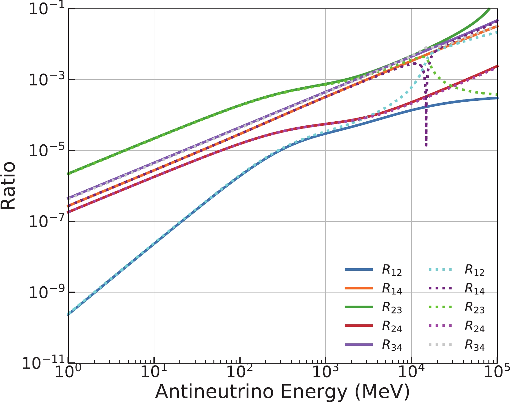
Figure B4. (color online) The values of the off-diagonal elements in
$ H^{\prime\prime} $ . The solid and dashed lines correspond to NH and IH, respectively. The input oscillation parameters are listed in Table 1.$ \begin{split} \widetilde{U}& \approx UR_{12}({\omega_1},{\phi_1})R_{23}({\omega_2},{\phi_2})\\& = \underbrace{R_{34}R_{24}R_{14}R_{23}R_{13}R_{12}}_{U} R_{12}({\omega_1},{\phi_1})R_{13}({\omega_2},{\phi_2}) \,, \end{split} \tag{B51a}$

(B51a) $ \Delta \widetilde{m}_{21}^2\approx\lambda_+-\lambda_-^\prime \,, \;\; \Delta \widetilde{m}_{31}^2\approx\lambda_{+}^{\prime}-\lambda_-^\prime \,, \;\; \Delta \widetilde{m}_{41}^2\approx H_{44}-\lambda_-^\prime \,. \tag{B52b}$

(B52b) -
Similar to the neutrino case, we combine
$ R_{12}(\theta_{12},0) $ and$ R_{12}({\omega_1},{\phi_1}) $ into one submatrix below:$ \begin{split} &R_{12}(\theta_{12},0)R_{12}({\omega_1},{\phi_1})\\ = & \begin{bmatrix} c_{12}&s_{12}&0&0\\ -s_{12}&c_{12}&0&0\\ 0&0&1&0\\ 0&0&0&1 \end{bmatrix} \begin{bmatrix} c_{{\omega_1}}&s_{{\omega_1}}{\rm e}^{-{\rm i}{\phi_1}}&0&0\\ -s_{{\omega_1}}{\rm e}^{{\rm i}{\phi_1}}&c_{{\omega_1}}&0&0\\ 0&0&1&0\\ 0&0&0&1 \end{bmatrix} \\ = & \begin{bmatrix} \widetilde{c}_{12}&\widetilde{s}_{12}{\rm e}^{-{\rm i}\widetilde{\delta}_{12}}&0&0\\ -\widetilde{s}_{12}{\rm e}^{{\rm i}\widetilde{\delta}_{12}}&\widetilde{c}_{12}&0&0\\ 0&0&1&0\\ 0&0&0&1 \end{bmatrix} \begin{bmatrix} {\rm e}^{{\rm i}\Theta_{12}}&0&0&0\\ 0&{\rm e}^{-{\rm i}\Theta_{12}}&0&0\\ 0&0&1&0\\ 0&0&0&1 \end{bmatrix} \\ = & R_{12}(\widetilde{\theta}_{12},\widetilde{\delta}_{12})D_{12}({\rm e}^{{\rm i}\Theta_{12}},{\rm e}^{-{\rm i}\Theta_{12}},1,1) \\ = & \widetilde{R}_{12}\,, \end{split}\tag{B53} $

(B53) with
${ \begin{split} & \widetilde{s}_{12} = \sin \widetilde{\theta}_{12} = \frac{|c_{12}\tan {\omega_1} {\rm e}^{{\rm i}{\phi_1}}+s_{12}|}{\sqrt{1+\tan^2 {\omega_1} }}\,, \\ & \widetilde{c}_{12} = \cos \widetilde{\theta}_{12} = \frac{|c_{12}-s_{12}\tan {\omega_1} {\rm e}^{{\rm i}{\phi_1}}|}{\sqrt{1+\tan^2 {\omega_1} }}\,, \end{split}} \tag{B54a}$

(B54a) $ {\rm e}^{{\rm i}\widetilde{\delta}_{12}} = \frac{(c_{12}\tan {\omega_1} {\rm e}^{{\rm i}{\phi_1}}+s_{12})(c_{12}-s_{12}\tan {\omega_1} {\rm e}^{-{\rm i}{\phi_1}})} {\cos \widetilde{\theta}_{12} \sin \widetilde{\theta}_{12} (1+\tan^2 {\omega_1}) } \,, \tag{B54b}$

(B54b) $ {\rm e}^{{\rm i}\Theta_{12}} = \frac{c_{12}-s_{12}\tan{\omega_1} {\rm e}^{\phi_1}}{\cos\widetilde{\theta}_{12}\sqrt{1+\tan^2{\omega_1}}} \,. \tag{B54c}$

(B54c) Therefore, we obtain
$ \widetilde{U}\approx R_{34}R_{24}R_{14}R_{23}R_{13}\widetilde{R}_{12}R_{13}({\omega_2},{\phi_2}) \,. \tag{B55}$

(B55) Here, we set a constraint on
$ \widetilde{\theta}_{12} $ within$ [0,\frac{\pi}{2}] $ .For further simplification, we exchange
$ \widetilde{R}_{12} $ and$ R_{13}({\omega_2},{\phi_2}) $ by$ \widetilde{R}_{12} R_{13}({\omega_2},{\phi_2})\approx R_{13}({\omega_2},{\phi_2})\widetilde{R}_{12}, \tag{B56}$

(B56) where
$ \begin{split}& \widetilde{R}_{12} R_{13}({\omega_2},{\phi_2}) = \\& \begin{bmatrix} \widetilde{c}_{12}c_{\omega_2}{\rm e}^{{\rm i}\Theta_{12}} & \widetilde{s}_{12}{\rm e}^{-{\rm i}(\widetilde{\delta}_{12}+\Theta_{12})} & \widetilde{c}_{12}s_{\omega_2} {\rm e}^{{\rm i} (\Theta_{12}-\phi_2 )} & 0 \\ -c_{\omega_2}\widetilde{s}_{12}{\rm e}^{{\rm i}(\widetilde{\delta}_{12}+\Theta_{12})} & \widetilde{c}_{12}{\rm e}^{-{\rm i}\Theta_{12}} & -\widetilde{s}_{12}s_{\omega_2}{\rm e}^{{\rm i}(\widetilde{\delta}_{12} + \Theta_{12} - \phi_2)} & 0 \\ -s_{\omega_2}{\rm e}^{{\rm i}\phi_2} & 0 & c_{\omega_2} & 0 \\ 0 & 0 & 0 & 1 \end{bmatrix}\,, \end{split}\tag{B57}$

(B57) and
$ R_{13}(\omega_2,\phi_2)\widetilde{R}_{12} $ yields$ \begin{split}& R_{13}(\omega_2,\phi_2)\widetilde{R}_{12} = \\& \begin{bmatrix} \widetilde{c}_{12}c_{\omega_2}{\rm e}^{{\rm i}\Theta_{12}} & c_{\omega_2}\widetilde{s}_{12} {\rm e}^{-{\rm i}(\widetilde{\delta}_{12}+\Theta_{12})} & s_{\omega_2}{\rm e}^{-{\rm i}\phi_2} & 0 \\ -\widetilde{s}_{12}{\rm e}^{{\rm i}(\widetilde{\delta}_{12}+\Theta_{12})} & \widetilde{c}_{12}{\rm e}^{-{\rm i}\Theta_{12}} & 0 & 0 \\ -\widetilde{c}_{12}s_{\omega_2} {\rm e}^{{\rm i}(\Theta_{12}+\phi_2)} & -\widetilde{s}_{12}s_{\omega_2}{\rm e}^{{\rm i}(\phi_2-\Theta_{12}-\widetilde{\delta}_{12})} & c_{\omega_2} & 0 \\ 0 & 0 & 0 & 1 \end{bmatrix}\,.\end{split} \tag{B58}$

(B58) Figure B5 quantifies the differences between all the elements of
$ \widetilde{R}_{12} R_{13}(\omega_2,\phi_2) $ and$ R_{13}(\omega_2,\phi_2)\widetilde{R}_{12} $ . It shows that the differences are allowable for exchange in the application range of our approximation.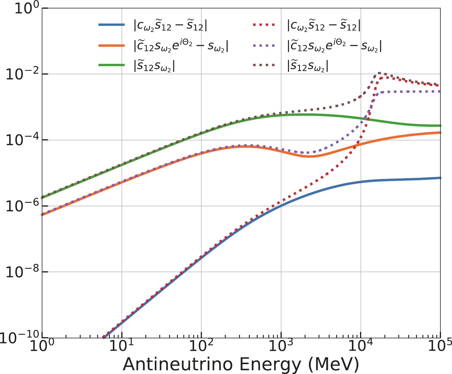
Figure B5. (color online) Differences between
$\widetilde{R}_{12}R_{23}(\omega_2, $ $ \phi_2) $ and$ R_{13}(\omega_2,\phi_2)\widetilde{R}_{12} $ . The solid and dashed lines correspond to NH and IH, respectively. The input oscillation parameters are listed in Table 1.Subsequently, we obtain the following approximate simplification over different E ranges:
$ \begin{split} \widetilde{U} & \approx R_{34}R_{24}R_{14}R_{13}R_{13}\widetilde{R}_{12} R_{13}({\omega_2},{\phi_2})\\ & = R_{34}R_{24}R_{14}R_{13}R_{13}R_{13}({\omega_2},{\phi_2})\widetilde{R}_{12}. \end{split} \tag{B59} $

(B59) It can be observed that
$ R_{13}(\theta_{13},0)R_{13}({\omega_2},{\phi_2}) $ can be simplified as$ \begin{split} &R_{13}(\theta_{13},0)R_{13}({\omega_2},{\phi_2})\\ = & \begin{bmatrix} c_{13}&0&s_{13}{\rm e}^{-{\rm i}\delta_{13}}&0\\ 0&1&0&0\\ -s_{13}{\rm e}^{{\rm i}\delta_{13}}&0&c_{13}&0\\ 0&0&0&1 \end{bmatrix} \begin{bmatrix} c_{{\omega_2}}&0&s_{{\omega_2}}{\rm e}^{-{\rm i}{\phi_2}}&0\\ 0&1&0&0\\ -s_{{\omega_2}}{\rm e}^{{\rm i}{\phi_2}}&0&c_{{\omega_2}}&0\\ 0&0&0&1 \end{bmatrix}\end{split} $

$ \begin{split}= & \begin{bmatrix} \widetilde{c}_{13}&0&\widetilde{s}_{13}{\rm e}^{-{\rm i}\widetilde{\delta}_{13}}&0\\ 0&1&0&0\\ -\widetilde{s}_{13}{\rm e}^{{\rm i}\widetilde{\delta}_{13}}&0&\widetilde{c}_{13}&0\\ 0&0&0&1 \end{bmatrix} \begin{bmatrix} {\rm e}^{{\rm i}\Theta_{13}}&0&0&0\\ 0&1&0&0\\ 0&0&{\rm e}^{-{\rm i}\Theta_{13}}&0\\ 0&0&0&1 \end{bmatrix} \\ = & R_{13}(\widetilde{\theta}_{13},\widetilde{\delta}_{13})D_{13}({\rm e}^{{\rm i}\Theta_{13}},1,{\rm e}^{-{\rm i}\Theta_{13}},1) \,,\end{split} \tag{B60}$

(B60) with
$ \begin{split} & \widetilde{s}_{13} = \sin \widetilde{\theta}_{13} = \frac{|c_{13}\tan {\omega_2} {\rm e}^{{\rm i}{\phi_2}}+s_{13}{\rm e}^{{\rm i}\delta_{13}}|} {\sqrt{1+\tan^2 {\omega_2} }} \,, \\ & \widetilde{c}_{13} = \cos \widetilde{\theta}_{13} = \frac{|c_{13}-s_{13}\tan {\omega_2} {\rm e}^{{\rm i}(\delta_{13}-{\phi_2})}|} {\sqrt{1+\tan^2 {\omega_2} }} \,, \end{split} \tag{B61a}$

(B61a) $ {\rm e}^{{\rm i}\widetilde{\delta}_{13}} = \frac{(c_{13}\tan {\omega_2} {\rm e}^{{\rm i}{\phi_2}}+s_{13}{\rm e}^{{\rm i}\delta_{13}})(c_{13}-s_{13}\tan {\omega_2} {\rm e}^{{\rm i}(\delta_{13}-{\phi_2})})} {\cos \widetilde{\theta}_{13} \sin \widetilde{\theta}_{13} (1+\tan^2 {\omega_2} )} \,, \tag{B61b}$

(B61b) $ {\rm e}^{{\rm i}\Theta_{13}} = \frac{c_{13}-s_{13}\tan{\omega_2} {\rm e}^{-{\rm i}(\delta_{13}-{\phi_2})}}{\cos\widetilde{\theta}_{13}\sqrt{1+\tan^2{\omega_2}}} \,. \tag{B61c}$

(B61c) We also set a bound on
$ \widetilde{\theta}_{13} $ within$ [0,\frac{\pi}{2}] $ . Subsequently, we obtain$ \widetilde{U}\approx R_{34}R_{24}R_{14}R_{13} R_{13}(\widetilde{\theta}_{13},\widetilde{\delta}_{13})D_{13} \widetilde{R}_{12} \,. \tag{B62}$

(B62) Similar to the approach in Eq. (85), we would like to exchange
$D_{13}({\rm e}^{{\rm i}\Theta_{13}},1,{\rm e}^{-{\rm i}\Theta_{13}},1)$ and$ \widetilde{R}_{12} $ using$ D_{13}({\rm e}^{{\rm i}\Theta_{13}},1,{\rm e}^{-{\rm i}\Theta_{13}},1) \widetilde{R}_{12} \approx \widetilde{R}_{12} D_{13}({\rm e}^{{\rm i}\Theta_{13}},1,{\rm e}^{-{\rm i}\Theta_{13}},1) \,, \tag{B63}$

(B63) where
$ D_{13}({\rm e}^{{\rm i}\Theta_{13}},1,{\rm e}^{-{\rm i}\Theta_{13}},1) \widetilde{R}_{12} = \begin{bmatrix} \widetilde{c}_{12}{\rm e}^{{\rm i}(\Theta_{12}+\Theta_{13})} & \widetilde{s}_{12}{\rm e}^{{\rm i}(\Theta_{13}-\widetilde{\delta}_{12}-\Theta_{12})} & 0 & 0 \\ -\widetilde{s}_{12} {\rm e}^{{\rm i}(\widetilde{\delta}_{12}+\Theta_{12})} & \widetilde{c}_{12}{\rm e}^{-{\rm i}\Theta_{12}} & 0 & 0 \\ 0 & 0 & {\rm e}^{-{\rm i}\Theta_{13}} & 0 \\ 0 & 0 & 0 & 1 \end{bmatrix} \tag{B64}$

(B64) and
$ \widetilde{R}_{12} D_{13}({\rm e}^{{\rm i}\Theta_{13}},1,{\rm e}^{-{\rm i}\Theta_{13}},1) = \begin{bmatrix} \widetilde{c}_{12}{\rm e}^{{\rm i}(\Theta_{12}+\Theta_{13})} & \widetilde{s}_{12}{\rm e}^{-{\rm i}(\widetilde{\delta}_{12}+\Theta_{12})} & 0 & 0 \\ -\widetilde{s}_{12} {\rm e}^{{\rm i}(\widetilde{\delta}_{12}+\Theta_{12}+\Theta_{13})} & \widetilde{c}_{12}{\rm e}^{-{\rm i}\Theta_{12}} & 0 & 0 \\ 0 & 0 & {\rm e}^{-{\rm i}\Theta_{13}} & 0 \\ 0 & 0 & 0 & 1 \tag{B65}\end{bmatrix}\,. $

(B65) Figure B6 shows the quantification of the negligible difference between
$D_{13}({\rm e}^{{\rm i}\Theta_{13}},1,{\rm e}^{-{\rm i}\Theta_{13}},1) \widetilde{R}_{12}$ and$\widetilde{R}_{12} D_{13}({\rm e}^{{\rm i}\Theta_{13}},1,{\rm e}^{-{\rm i}\Theta_{13}},1)$ . Again, it can be observed that the differences are quite small.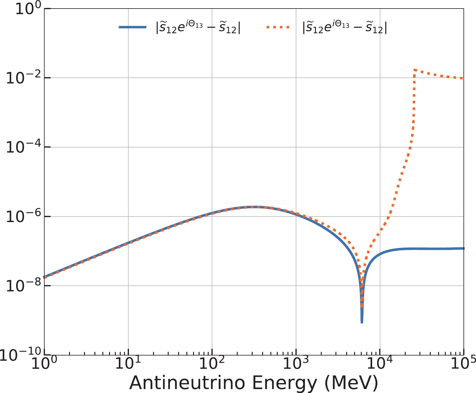
Figure B6. (color online) Differences between
$D_{13}({\rm e}^{{\rm i}\Theta_{13}},1, $ ${\rm e}^{-{\rm i}\Theta_{13}},1)\widetilde{R}_{12}$ and$\widetilde{R}_{12} D_{13}({\rm e}^{{\rm i}\Theta_{13}},1,{\rm e}^{-{\rm i}\Theta_{13}},1)$ . The solid and dashed lines correspond to NH and IH, respectively. The input oscillation parameters are listed in Table 1.Consequently, the effective mixing matrix can be written as
$ \widetilde{U}\approx R_{34}R_{24}R_{14}R_{13} R_{13}(\widetilde{\theta}_{13},\widetilde{\delta}_{13}) R_{12}(\widetilde{\theta}_{12},\widetilde{\delta}_{12}) D_{123} \tag{B66}$

(B66) with
$ D_{123} = D_{123}({\rm e}^{{\rm i}(\Theta_{12}+\Theta_{13})},{\rm e}^{-{\rm i}\Theta_{12}},{\rm e}^{-{\rm i}\Theta_{13}},1) \,. \tag{B67}$

(B67) Similarly, here
$D_{123}({\rm e}^{{\rm i}(\Theta_{12}+\Theta_{13})},{\rm e}^{-{\rm i}\Theta_{12}},{\rm e}^{-{\rm i}\Theta_{13}},1)$ can be cancelled like the Majorana phases when neutrinos oscillate. Eventually, the effective mixing matrix$ \widetilde{U} $ is identical to the vacuum case U except for an additional$ \widetilde{\delta}_{12} $ .$ \widetilde{U} $ can be written as$ \widetilde{U}\approx R_{34}R_{24}R_{14}R_{13} R_{13}(\widetilde{\theta}_{13},\widetilde{\delta}_{13}) R_{12}(\widetilde{\theta}_{12},\widetilde{\delta}_{12}) \,. \tag{B68}$

(B68) Similarly, we conclude that
$ \widetilde{\theta}_{12} = \theta_{12}+\omega_1 $ ,$ \widetilde{\theta}_{13} = \theta_{13}+{\omega_2} $ ,$ \widetilde{\delta}_{13} = \delta_{13} $ , and$ \widetilde{\delta}_{12} = \Theta_{12} = \Theta_{13} = 0 $ when$ \delta_{13} = \delta_{24} = \delta_{34} = 0 $ . It is now much easier to diagonalize the effective Hamiltonian because it is a real Hermitian matrix. For real matrices, the Jacobi-like method reduces to the Jacobi method. -
In this subsection, we summarize the effective mixing matrix
$ \widetilde{U} $ for both the neutrino and antineutrino cases based on the results of B.1 and B.2 in Table B1. Using the neutrino oscillation probability functions in Eq. (9) and the elements in Table B1, every neutrino oscillation probability is available.$\alpha$ 

$\widetilde{U}_{\alpha i}$ 

- e $\widetilde{U}_{e1}$ 

$\widetilde{c}_{12}\widetilde{c}_{13}c_{14}$ 

$\widetilde{U}_{e2}$ 

$\widetilde{c}_{13}c_{14}\widetilde{s}_{12}{\rm e}^{-{\rm i}\widetilde{\delta}_{12} }$ 

$\widetilde{U}_{e3}$ 

$c_{14}\widetilde{s}_{13}{\rm e}^{-{\rm i}\widetilde{\delta}_{13} }$ 

$\widetilde{U}_{e4}$ 

$s_{14}$ 

$\mu$ 

$\widetilde{U}_{\mu1}$ 

$-\widetilde{s}_{12}c_{23}c_{24}{\rm e}^{{\rm i}\widetilde{\delta}_{12} }-\widetilde{c}_{12}(\widetilde{s}_{13}c_{24}s_{23}{\rm e}^{{\rm i}\widetilde{\delta}_{13} }+\widetilde{c}_{13}s_{14}s_{24}{\rm e}^{-{\rm i}\delta_{24} })$ 

$\widetilde{U}_{\mu2}$ 

$\widetilde{c}_{12}c_{23}c_{24}-\widetilde{s}_{12}(\widetilde{s}_{13}c_{24}s_{23}{\rm e}^{{\rm i}\widetilde{\delta}_{13} }+\widetilde{c}_{13}s_{14}s_{24}{\rm e}^{-{\rm i}\delta_{24} }){\rm e}^{-{\rm i}\widetilde{\delta}_{12} }$ 

$\widetilde{U}_{\mu3}$ 

$\widetilde{c}_{13}c_{24}s_{23}-\widetilde{s}_{13}s_{14}s_{24}{\rm e}^{-{\rm i}\widetilde{\delta}_{13} }{\rm e}^{-{\rm i}\delta_{24} }$ 

$\widetilde{U}_{\mu4}$ 

$c_{14}s_{24}{\rm e}^{-{\rm i}\delta_{24} }$ 

$\tau$ 

$\widetilde{U}_{\tau1}$ 

$ \widetilde{c}_{12}[\widetilde{s}_{13}(s_{23}s_{24}s_{34}{\rm e}^{{\rm i}\delta_{24} }{\rm e}^{-{\rm i}\delta_{34} }-c_{23}c_{34}){\rm e}^{{\rm i}\widetilde{\delta}_{13} }-\widetilde{c}_{13}c_{24}s_{14}s_{34}{\rm e}^{-{\rm i}\delta_{34} }] \widetilde{s}_{12}(c_{34}s_{23}+c_{23}s_{24}s_{34}{\rm e}^{{\rm i}\delta_{24} }{\rm e}^{-{\rm i}\delta_{34} }){\rm e}^{{\rm i}\widetilde{\delta}_{12} } $ 

$\widetilde{U}_{\tau2}$ 

$ \widetilde{s}_{12}[\widetilde{s}_{13} (s_{23}s_{24}s_{34}{\rm e}^{{\rm i}\delta_{24} }{\rm e}^{-{\rm i}\delta_{34} }-c_{23}c_{34}){\rm e}^{{\rm i}\widetilde{\delta}_{13} } -\widetilde{c}_{13}c_{24}s_{14}s_{34}{\rm e}^{-{\rm i}\delta_{34} }]{\rm e}^{-{\rm i}\widetilde{\delta}_{12} } -\widetilde{c}_{12}(c_{34}s_{23}+c_{23}s_{24}s_{34}{\rm e}^{{\rm i}\delta_{24} }{\rm e}^{-{\rm i}\delta_{34} }) $ 

$\widetilde{U}_{\tau3}$ 

$\widetilde{c}_{13}(c_{23}c_{34}-s_{23}s_{24}s_{34}{\rm e}^{{\rm i}\delta_{24} }{\rm e}^{-{\rm i}\delta_{34} })-\widetilde{s}_{13}c_{24}s_{14}s_{34}{\rm e}^{-{\rm i}\widetilde{\delta}_{13} }{\rm e}^{-{\rm i}\delta_{34} }$ 

$\widetilde{U}_{\tau4}$ 

$c_{14}c_{24}s_{34}{\rm e}^{-{\rm i}\delta_{34} }$ 

s $\widetilde{U}_{s1}$ 

$\begin{aligned} \widetilde{c}_{12}[\widetilde{s}_{13}(c_{34}s_{23}s_{24}{\rm e}^{{\rm i}\delta_{24} }+c_{23}s_{34}{\rm e}^{{\rm i}\delta_{34} }){\rm e}^{{\rm i}\widetilde{\delta}_{13} }-\widetilde{c}_{13}c_{24}c_{34}s_{14}]+ \widetilde{s}_{12}(c_{23}c_{34}s_{24}{\rm e}^{{\rm i}\delta_{24} }-s_{23}s_{34}{\rm e}^{{\rm i}\delta_{34} }){\rm e}^{{\rm i}\widetilde{\delta}_{12} } \end{aligned}$ 

$\widetilde{U}_{s2}$ 

$\widetilde{s}_{12}[\widetilde{s}_{13} (c_{34}s_{23}s_{24}{\rm e}^{{\rm i}\delta_{24} }+c_{23}s_{34}{\rm e}^{{\rm i}\delta_{34} }){\rm e}^{{\rm i}\widetilde{\delta}_{13} }-\widetilde{c}_{13}c_{24}c_{34}s_{14}]{\rm e}^{-{\rm i}\widetilde{\delta}_{12} } +\widetilde{c}_{12}(s_{23}s_{34}{\rm e}^{{\rm i}\delta_{34} }-c_{23}c_{34}s_{24}{\rm e}^{{\rm i}\delta_{24} }) $ 

$\widetilde{U}_{s3}$ 

$-\widetilde{c}_{13}(c_{34}s_{23}s_{24}{\rm e}^{{\rm i}\delta_{24} }+c_{23}s_{34}{\rm e}^{{\rm i}\delta_{34} })-c_{24}c_{34}s_{14}{\rm e}^{-{\rm i}\widetilde{\delta}_{13} }$ 

$\widetilde{U}_{s4}$ 

$c_{14}c_{24}c_{34}$ 

Table B1. The elements of the effective mixing matrix for the 3+1-neutrino case in matter based on the results from section B.1 and B.2. If the sterile parameters are set to zero, this mixing will reduce to the effective mixing matrix for 3-flavor neutrinos with the matter effect.
A compact analytical approximation for a light sterile neutrino oscillation in matter
- Received Date: 2020-03-30
- Accepted Date: 2020-06-23
- Available Online: 2020-10-01
Abstract: The existence of light sterile neutrinos is a long-standing question in particle physics. Several experimental “anomalies” might be explained by introducing eV mass scaled light sterile neutrinos. Many experiments are actively searching for such light sterile neutrinos through neutrino oscillation. For long baseline experiments, the matter effect should be treated carefully for precise calculation of the neutrino oscillation probabilities. However, this is usually time-consuming or analytically complex. In this manuscript, we adopt a Jacobi-like method to diagonalize the Hermitian Hamiltonian matrix and derive analytically simplified neutrino oscillation probabilities for 3 (active) + 1 (sterile)-neutrino mixing for a constant matter density. These approximations can reach a considerably high numerical accuracy while retaining their analytical simplicity and fast computing speed. This would be useful for current and future long baseline neutrino oscillation experiments.


 DownLoad: