


 Abstract
 HTML
HTML Reference
 Related
 PDF
PDF


-
One of the greatest challenges in modern cosmology is the late-time comportment of our Universe. We use several sets of high-precision observational data gathered from various cosmic sources such as the Cosmic Microwave Background (CMB) [1-3], SuperNova type Ia (SNe Ia) [4-8], Large Scale Structure (LSS) [9-11], Weak Lensing (WL) [12], and Baryon Acoustic Oscillations (BAO) [13] as standard candles, which discovered that our Universe is undergoing accelerated expansion. The fascinating part is that the expansion of the Universe is believed to be caused by an obscure energy termed dark energy, which is equal to approximately two-thirds of the complete energy budget of the Universe. Owing to the puzzling nature of the dark sector (dark energy (DE) and dark matter (DM); DE yields a late-time speeding up of the cosmological foundation, whereas DM carries on as undetectable residue matter supporting the procedure of gravitational clustering) and the fact that their existence is construed only through their gravitational impact, it is essential to verify whether there is a need to contemplate these elements, regardless of whether there is any deflection from the ordinary general relativity (GR) theory on enormous scales. Using Einstein's field equations (EFEs), one can realize the existence of an accelerated expansion portrayed by a positive constant, which is extremely small, in the edge work of GR, referred to as the
$ \Lambda - $ CDM model [14]. In the present situation, this small positive constant is related to dark energy in the void space, which is utilized to clarify the ongoing coeval accelerating expansion of the Universe against the alluring impacts of gravity. In general, there are two main methodologies that could explain the theory behind the accelerated expansion of the Universe. The first methodology involves altering the matter substance of the Universe by introducing a DE area, beginning either with a phantom field, a standard scalar field, or a mixture of the two fields in a unified model and then progressing toward more complicated scenarios; see [15-17] and the references therein for more subtleties and audits. The second methodology involves modifying the gravitational area itself (see, e.g., [18-21]), which can likewise be well-respected as one of the significant theories for clarifying the accelerated expansion of the Universe. We are prompted by this basic hypothesis that at significant astrophysical and cosmological scales, the usual GR may not depict the dynamical evolution of the Universe effectively. Several endeavors have been made to manage this problem, among which gravity theories about broadening GR have aroused much enthusiasm over the previous decades. With regard to the modified gravity theories, DM can be geometrically depicted and the accelerated expansion at late times can be explained. Thus, the cosmological constant issue may be settled (for an exhaustive dynamical system investigation of some cosmological models in terms of alternative gravitational theories, see [22-32]). Among the various models of DE, the altered gravity models are very fascinating, as they integrate some movements of the quantum and general gravity theories. Different techniques have been suggested until now to modify the gravitational action (see [33] for more details), leading to various classes of alternative gravitational theories. In this regard, some leading models incorporate$ f(R) $ gravity [19, 21, 34-53],$ f(T) $ gravity [54-58],$ f({\cal{T}}) $ gravity [59, 60],$ f({\cal{G}}) $ gravity [61-63],$ f(R, T) $ gravity [64-80],$ f({\cal{T}}, T) $ gravity [81-86], and$ f(R, {\cal{G}}) $ gravity [87], where R, T,$ {\cal{T}} $ , and$ {\cal{G}} $ are Ricci's scalar, trace of stress-energy tensor, torsion scalar, and Gauss-Bonnet scalar, respectively. In$ f(R) $ gravity theory, the general expression of the Ricci scalar$ R = g^{\mu \nu}R_{\mu \nu} $ is utilized to a greater extent instead of R, though$ f(T) $ gravity is a general type of teleparallel gravity. Spurred by the achievement of the cosmological constant as a straightforward and significant candidate for DE and DM, a few matter fields are combined with the expression of the Ricci scalar R in the action geometry sector in some alternative theories of gravitation (e.g.,$ f(R, {\cal{L}}_m) $ theory, where$ {\cal{L}}_m $ is the matter Lagrangian density).In the interest of including certain components of matter into the geometry of action, the
$ f(R, T) $ theory was suggested in [88], and it has generally been a fascinating framework for studying acceleration models. The$ f(R, T) $ gravity theory generalizes$ f(R) $ gravity theories by introducing the trace of the stress-energy tensor added to the Ricci scalar. The validation for the reliance on T originates from enlistments emerging from a few exotic fluid or quantum impacts. This enlistment perspective essentially encompasses or connects to the recommendations mentioned; for instance, geometrical curvature prompting matter, geometrical portrayal of physical powers, and a geometrical source for the matter substance of the Universe. In Ref. [91], the field equations of a few specific models are introduced; in particular, scalar field models$ f(R, T^{\Phi}) $ are examined in detail along with a concise account of their cosmological ramifications. Similarly, the motion equation of the test particle and the Newtonian boundary of this equation are also studied in Ref. [88]. Until now, the following problems have been explored along with this alternative theory: thermodynamics [89-91], energy conditions [92], anisotropic cosmology [93, 94], cosmology in which the portrayal uses an assistive scalar field [95], reconstruction of some cosmological models [96], wormhole solution [97, 98], scalar perturbations [99], and some other relevant aspects [80, 100-102]. In addition, a further generalization of this theory has been suggested recently in Refs. [103, 104].Consequently, it is not reasonable to affirm or refute such theories depending on the outcomes of cosmology and contrast them with observed datum; for instance, the challenge of the viability of
$ f(R, T) $ as an alternative modification of gravity, as discussed in [105]. In any case, to set up an agreeable theory of gravitation, it is essential to consider it at the astrophysical level, for instance, by utilizing relativistic stellar structures. A few contentions for these modified theories originate from the presumption that relativistic stellar structures in the powerful gravitational sector could distinguish common gravity from its generalizations. In the scenario of$ f(R,T) $ gravity, an enormous number of contributions on the evolution of compact stellar structures are accessible in the literature. In this context, the hydrostatic equilibrium structure of strange stars and neutron stars have been investigated [73]. The configuration of compact stellar structures in$ f(R,T) $ gravity was explored recently in Refs. [67, 68, 71, 106-108], though gravastars (GRAvitational VAcuum STARS) resolution has been obtained in [109-111].The distribution of anisotropic fluids plays a significant role in the understanding of the internal geometry and evolutionary phases of relativistic stellar structures. As compact stellar systems have ultradense cores and their density surpasses nuclear density, the pressure inside compact stellar systems ought to be anisotropic [112]. In anisotropic relativistic astrophysical systems, it is seen that the pressure is resolved into its radial and tangential components. Under this specific circumstance, numerous researchers have explored the attributes of compact and dense stellar systems involving anisotropic fluid structure. Ruderman [113] first proposed the concept of anisotropy for static spherically symmetric structures and, subsequently, numerous astrophysicists have included this parameter while modeling compact stellar structures. As a compact stellar structure is shaped with very dense matter, a very high magnetic domain is related with it owing to the principle of magnetic flux preservation. The enormous magnetic domain may produce pressure anisotropy inside the stellar structure [114]. Higher densities may similarly prompt anisotropy [115-119]. Thus, the anisotropy aspect is another factor that is incorporated in EFEs, leading to progressively realistic models of the spherically symmetric compact stellar structures. If the anisotropy parameter is positive, an outward repulsive force will be applied on the stellar structure, making it increasingly compact and steady. The primary explanation behind the emerging anisotropy in an
$ f(R, T) $ gravity theory model could be the anisotropic nature of the two-fluid system without interaction. Further, it ought to be emphasized that from a quantum point of view, the$ T- $ dependent Lagrangian might be identified with the formation of particles that normally portray the presence of bulk viscosity and other flaws in the alluded fluid. Consequently, we suggest models in which the transverse pressure surpasses the radial pressure. To determine accurate solutions of EFEs, two dissimilar methodologies are frequently employed: it is possible that we determine the space--time metric elements first and then establish the matter profile; alternatively, we may first portray the material features in terms of certain state equations, i.e., the relationship in the form$ p = p(\rho) $ , and subsequently investigate the metric potentials. While searching for a well-defined solution, the constants arising in the solution perform a significant role. A slight difference in the values of the constants can distance the stellar structure from its position of equilibrium. Therefore, several authors have studied compact stellar structure models by employing the Karmarkar condition. At present, when the Karmarkar condition [120] is being attempted on the gravitational components$ g_{rr} $ and$ g_{tt} $ , the issue of establishing the spatiotemporal elements obtained make simple to a great area, and the four-dimensional Riemannian spatiotemporal variety can be described graphically in the five-dimensional pseudo-Euclidean spatiotemporal variety without any change in its intrinsic characteristics. The solutions fulfilling the Karmarkar conditions alongside the condition suggested by Pandey & Sharma [ 121] are well-known as embedding class-one solutions. It is intriguing to observe that Schwarzschild's internal solution [122] is the only structure of bounded neutral matter with a disappearing anisotropy parameter fulfilling the Karmarkar condition. For a further in-depth survey, one may refer to the literature [123, 124-125], where the authors have clearly examined the impacts of the procedure of embedding four-dimensional Riemannian spatiotemporal variety into five-dimensional pseudo-Euclidean spatiotemporal variety in the scenario of GR and alternative gravity.In this study, we examine anisotropic spherically symmetric solutions in the domain of alternative gravity theories, particularly, the
$ f(R, T) $ theory of gravity. In this respect, we consider that the matter Lagrangian density$ {\cal{L}}_m $ (defined as$ {\cal{L}}_m = -{\cal{P}} = (p_r+2p_t)/3 $ , i.e., the isotropic pressure) can be asserted as a linear function of the Ricci scalar R and the trace of the energy--momentum tensor T, i.e.,$ f(R, T) = R + 2\chi T $ , where$ \chi $ is a dimensionless coupling constant, to depict the global set of modified EFEs for anisotropic matter distribution. We also consider the embedding class I procedure by embedding four-dimensional space--time into a five-dimensional flat Euclidean space to obtain a complete space--time representation in the interior of the relativistic stellar system. Moreover, for investigating the physical availability of the acquired solutions, we have analyzed four different compact stars, namely, PSR J1614-2230, Vela X-1, Cen X-3, and SAX J1808.4-3658 with linked physical parameters analytically and graphically. Accordingly, the familiar Darmois--Israel [126, 127] coordinating conditions can be used to calculate all the physical and constant ingredients of the stellar system.This paper is organized as follows: Beginning with a brief introduction in Section 1, we review the concept of
$ f(R,T)- $ gravity theory in Section 2. In Section 3, the basic EFEs for anisotropic matter distributions in$ f(R, T)- $ gravity are described. In Section 4, we will describe the Karmarkar condition, which is well known as an embedding class-one solution. Thereafter, in Section 5, we present the formulation of the complete stellar system under the embedding class-one technique in the area of$ f(R, T)- $ gravity and its thermodynamic description. In Section 6, we analyze the new solutions through various physical tests such as hydrostatic equilibrium, causality condition, stability factor, adiabatic index and stability, static stability criterion, and energy conditions. In Section 7, we coordinate the acquired stellar system with the external space--time described by the Schwarzschild metric to obtain the constant parameters. Furthermore, the stiffness of the EoS and the$ M-R $ and$ I-M $ diagrams are discussed in Section 8. Finally, we conclude our investigation with a short discussion of the result in Section 9. -
In the Einstein--Hilbert action, if the Ricci scalar R is replaced by a function of R and the trace of the stress--energy tensor T, the modified action in
$ f(R,T)- $ gravity is expressed as$ S = \frac{1}{16\pi}\int f(R,T)\sqrt{-g}\; {\rm d}^{4}x+\int {\cal{L}}_{m}\sqrt{-g}\; {\rm d}^{4}x, $

(1) where det
$ (g_{\mu \nu}) = g $ . The source term of the matter Lagrangian density$ {\cal{L}}_m $ defines a stress tensor as$ T_{\mu\nu} = -\frac{2}{\sqrt{-g}}\,\frac{\delta \big(\sqrt{-g}\,{\cal{L}}_m \big)}{\delta g^{\mu\nu}}. $

(2) Following Harko et al.'s approach [88], Eq. (2) reduces to
$ T_{\mu\nu} = g_{\mu\nu} {\cal{L}}_m-2\frac{\partial {\cal{L}}_m}{\partial g^{\mu\nu}}. $

(3) Variation in the action with respect to
$ g_{\mu \nu} $ yields the field equations$ \begin{split}& \left( R_{\mu\nu}- \nabla_{\mu} \nabla_{\nu} \right)f_R (R,T) +g_{\mu\nu} \Box f_R (R,T) - \frac{1}{2} f(R,T)g_{\mu\nu} \\ &\quad = 8\pi \; T_{\mu\nu} - f_T (R,T)\; \Big( T_{\mu\nu}+\Theta_{\mu \nu} \Big), \end{split} $

(4) provided
$ f_R (R,T) = {\partial f(R,T)}/{\partial R} $ and$f_T (R,T) = {\partial f(R, T)}/ {\partial T}$ .$ \nabla_\mu $ denotes the covariant derivative, whereas the box operator$ \Box $ is defined as$ \Box \equiv {1 \over \sqrt{-g}} {\partial \over \partial x^\mu}\left(\sqrt{-g}\; g^{\mu\nu} {\partial \over \partial x^\nu} \right) $

with
$ \Theta_{\mu\nu} = g^{\alpha\beta} {\delta T_{\alpha\beta} \over \delta g^{\mu\nu}}. $

The conservation equation [128] yields
$ \begin{split} \nabla^{\mu}T_{\mu\nu} =& \frac{f_T(R, T)}{8\pi -f_T(R,T)}\bigg[(T_{\mu\nu}+\Theta_{\mu\nu})\nabla^{\mu}\ln f_T(R,T) \\ &+\nabla^{\mu}\Theta_{\mu\nu}-\frac{1}{2}g_{\mu\nu}\nabla^{\mu}T\bigg]. \end{split} $

(5) Therefore,
$ \nabla^{\mu}T_{\mu\nu} \neq 0 $ implies that the conservation equation no longer holds in$ f(R,T) $ theory. Using Eq. (3), the tensor$ \Theta_{\mu\nu} $ is found to be$ \Theta_{\mu\nu} = - 2 T_{\mu\nu} +g_{\mu\nu}{\cal{L}}_m - 2g^{\alpha\beta}\,\frac{\partial^2 {\cal{L}}_m}{\partial g^{\mu\nu}\,\partial g^{\alpha\beta}}.\; \; \; $

(6) To complete the field equations, we assume an anisotropic fluid source
$ T_{\mu\nu} = (\rho+p_r) u_\mu u_\nu-p_t g_{\mu\nu}+(p_r-p_t)g_{v_\mu v_\nu}, $

(7) where
$ {u_{\nu}} $ is the four-velocity, satisfying$ u_{\mu}u^{\mu} = -1 $ and$ u_{\nu}\nabla^{\mu}u_{\mu} = 0 $ ,$ \rho $ is the matter density, and$ p_r $ and$ p_t $ are the radial and transverse pressures, respectively. If we define the isotropic pressure as$ -{\cal{P}} = {\cal{L}}_m = (p_r+2p_t)/3 $ [88], then Eq. (6) reduces to$ \Theta_{\mu\nu} = -2T_{\mu\nu}-{\cal{P}}g_{\mu \nu}. $

(8) Further, the functional
$ f(R,T) $ is chosen to be$ f(R,T) = R+2\chi T $ [88], where$ \chi $ is the coupling constant. Now the field equations (5) take the form$ G_{\mu\nu} = 8\pi \; T_{\mu\nu}+\chi T\; g_{\mu\nu}+2\chi(T_{\mu\nu}+{\cal{P}}g_{\mu\nu}). $

(9) For
$ \chi = 0 $ , one can recover the general relativistic field equations. The linear expression in$ f(R,T) $ solves several cosmological and astrophysical related problems. By substituting$ f(R,T) = R+2\chi T $ and Eq. (8) in Eq. (5), we obtain$ \nabla^{\mu}T_{\mu\nu} = -\frac{\chi}{2(4\pi+\chi)}\bigg[g_{\mu\nu}\nabla^{\mu}T+2\,\nabla^{\mu} \big({\cal{P}} g_{\mu\nu} \big)\bigg]. $

(10) Thus, the conservation equation in Einstein's gravity can be recovered for
$ \chi = 0 $ . -
To determine the field equations we assume an interior space-time of the form
$ {\rm d}s_-^2 = {\rm e}^\nu {\rm d}t^2 - {\rm e}^\lambda {\rm d}r^2 - r^2 ({\rm d}\theta^2 + \sin ^2 \theta \; {\rm d}\phi^2). $

(11) For the space-time expressed in Eq. (11), the field equation (9) becomes
$ 8\pi \rho_{\rm eff} = {\rm e}^{-\lambda} \left({\lambda' \over r}-{1 \over r^2} \right)+{1 \over r^2}, $

(12) $ 8\pi p_{r{\rm eff}} = {\rm e}^{-\lambda} \left({\nu' \over r}+{1 \over r^2} \right)-{1 \over r^2}, $

(13) $ 8\pi p_{t{\rm eff}} = {{\rm e}^{-\lambda} \over 4}\left(2\nu''+\nu'^2+{2(\nu'-\lambda') \over r}-\nu' \lambda' \right), $

(14) where
$ \begin{split} \rho_{\rm eff} =& \rho+{\chi \over 24\pi} \Big(9\rho-p_r-2p_t\Big), \\ p_{r{\rm eff}} =& p_r-{\chi \over 24\pi} \Big(3\rho-7p_r-2p_t \Big), \\ p_{t{\rm eff}} =& p_t-{\chi \over 24\pi} \Big(3\rho-p_r-8p_t \Big). \end{split} $

Now the decoupled field equations (12)-(14) are as follows:
$ \begin{split} \rho =& \frac{{\rm e}^{-\lambda}}{48 r^2 (\chi +2 \pi ) (\chi +4 \pi )} \Big[r \lambda ' \left\{16 (\chi +3 \pi )-r \chi \nu '\right\} \\ &+ 16 (\chi +3 \pi ) ({\rm e}^{\lambda}-1) +r \chi \left\{2 r \nu ''+\nu ' \left(r \nu '+4\right)\right\} \Big], \end{split} $

(15) $ \begin{split} p_r =& \frac{{\rm e}^{-\lambda}}{48 r^2 (\chi +2 \pi ) (\chi +4 \pi )} \Big[r \big\{\chi \lambda ' (r \nu '+8)-2 r \chi \nu '' \\ &+ \nu ' \left(20 \chi-r \chi \nu '+48 \pi \right)\big\} -16 (\chi +3 \pi )(e^{\lambda}-1) \Big], \end{split} $

(16) $ \begin{split} p_t =& \frac{{\rm e}^{-\lambda}}{48 r^2 (\chi +2 \pi ) (\chi +4 \pi )} \Big[r \Big\{-\lambda ' \big\{r (5 \chi +12 \pi ) \nu ' \\ &+ 4 (\chi +6 \pi )\big\}+2 r (5 \chi +12 \pi ) \nu '' +r (5 \chi +12 \pi ) \nu '\; ^2 \\&+ 8 (\chi +3 \pi ) \nu '\Big\}+ 8 \chi \left({\rm e}^{\lambda }-1\right) \Big] . \end{split} $

(17) To solve the field equations, we have to assume some of the physical quantities that satisfy strict physical constraints.
-
The Kasner coordinate transformation [129] shows that the exterior Schwarzschild vacuum is class-two space--time. Using the following transformations,
$ \begin{split} X = &{R \sin t \over \sqrt{R^2+16m^2}},\; Y = {R \cos t \over \sqrt{R^2+16m^2}}, \\ Z =& \int \sqrt{1+{256m^4 \over (R^2+16m^2)^3}}\; {\rm d}R, \end{split} $

where
$ R = \sqrt{8m(r-2m)} $ and$ r^2 = x^2+y^2+z^2 $ , the well-known Schwarzschild vacuum reduces to$ {\rm d}s^2 = -{\rm d}x^2-{\rm d}y^2-{\rm d}z^2+{\rm d}X^2+{\rm d}Y^2-{\rm d}Z^2. $

(18) This means that the Schwarzschild exterior space--time can be embedded into a six-dimensional pseudo-Euclidean manifold. This method was extended for the general four-dimensional space--time of the form (11) by Gupta & Goel [ 130]. The chosen coordinate transformations were
$ \begin{split} z_1 =& k{\rm e}^{\nu/2} \cosh \left({t \over k}\right),\; z_2 = k{\rm e}^{\nu/2} \sinh \left({t \over k}\right),\; z_3 = f(r), \\ z_4 =& r \sin \theta \cos \phi ,\; z_5 = r \sin \theta \sin \phi,\; z_6 = r \cos \theta, \end{split} $

which transform (11) into
$ {\rm d}s^2 = ({\rm d}z_1)^2-({\rm d}z_2)^2 \mp ({\rm d}z_3)^2-({\rm d}z_4)^2-({\rm d}z_5)^2-({\rm d}z_6)^2, $

(19) with
$ [f'(r)]^2 = \mp \big[-\big({\rm e}^\lambda-1 \big)+k^2 {\rm e}^\nu \nu'^2/4 \big] $ .Equation (19) also implies that the interior line element (11) can be embedded in six-dimensional pseudo-Euclidean space. However, if
$ ({\rm d}z_3)^2 = [f'(r)]^2 = 0 $ , it can be embedded in 5D Euclidean space, i.e.,$ [f'(r)]^2 = \mp \Big[-\big({\rm e}^\lambda-1 \big)+{k^2 {\rm e}^\nu \nu'^2 \over 4} \Big] = 0, $

(20) which implies
$ {\rm e}^\lambda = 1+{k^2 \over 4}\; \nu'^2 {\rm e}^\nu $

(21) i.e., Eq. (19) reduces to
$ {\rm d}s^2 = ({\rm d}z_1)^2-({\rm d}z_2)^2 -({\rm d}z_4)^2-({\rm d}z_5)^2-({\rm d}z_6)^2, $

(22) a class-one spacetime.
The same condition (21) was originally derived by Karmarkar [120] in the form of the components of the Riemann tensor as
$ R_{rtrt}R_{\theta \phi \theta \phi} = R_{r\theta r \theta}R_{\phi t \phi t}+R_{r \theta \theta t}R_{r \phi \phi t}. $

(23) Pandey & Sharma [ 121] pointed out that the Karmarkar condition is only a necessary condition to become class one; they discovered the sufficient condition as
$ R_{\theta \phi \theta \phi}\ne 0 $ . Hence, the necessary and sufficient condition to be a class one is to satisfy both the Karmarkar and Pandey-Sharma conditions. In terms of the metric components, Eq. (23) can be written as$ {2\nu'' \over \nu'}+\nu' = {\lambda' {\rm e}^\lambda \over {\rm e}^\lambda -1}, $

(24) which, on integration, becomes the following:
$ {\rm e}^{\nu} = \left(A+B\int \sqrt{{\rm e}^{\lambda}-1}\; {\rm d}r\right)^2. $

(25) where A and B are the constants of integration. In general relativity, there is no class-one exterior, as the existing Schwarzschild's exterior itself is a class-two space-time. It has been shown that the two class-one isotropic-neutral solutions in general relativity, i.e., the Schwarzschild uniform density model and Kohler-Chao infinite boundary model are the only two possible solutions [131]. However, Mustafa et al. [132] have also shown that these two isotropic-neutral solutions still exist in
$ f(R,T)- $ theory as well, although the constant density model in GR can have decreasing density in$ f(R,T)- $ gravity and the infinite boundary Kohler-Chao solution can have a finite boundary, where the pressure vanishes owing to the$ f(R,T)- $ term.Once one of the metric functions is determined, say, for
$ {\rm e}^\lambda $ , then the EoS is fixed. Using Eqs. (12), (13), and (25), we obtain$ \begin{split} 8\pi p_{r{\rm eff}} =& -{1 \over r^2}+\bigg[{c_1 \over r}+{1 \over r^2}\int \left(1-8\pi r^2 \rho_{\rm eff} \right){\rm d}r \bigg]. \\ & \bigg[{2B \sqrt{{\rm e}^\lambda-1} \over r(A+B \int \sqrt{{\rm e}^\lambda-1}\; {\rm d}r)} +{1 \over r^2}\bigg]. \end{split} $

(26) However, because of the highly coupled and nonlinear field equations (15)-(17), finding an exact expression for the EoS in terms of
$ p_r $ and$ \rho $ is very difficult; instead, one can represent it graphically . -
Solving the field equations in
$ f(R,T)- $ gravity exactly is a challenging task because of the highly coupled nonlinear differential equations. To simplify the problem, we have adopted the embedding class-one approach, which is an application of four-dimensional space-time. Here, we propose a new metric function:$ {\rm e}^\lambda = 1+a r^2 {\rm e}^{b r^2+c r^4}. $

(27) The physical motivation for using this ansatz is that it not only is a new metric function but also satisfies the required criteria of
$ g_{rr} $ , i.e.,$ {\rm e}^{\lambda(0)} = 1 $ , and being an increasing function of r. Satisfying these properties increases the probability of obtaining well-behaved solutions.Using Eq. (27) in Eq. (25), we get
$ {\rm e}^\nu = \left[A+\frac{B}{\sqrt{2 c}}\; \sqrt{a {\rm e}^{b r^2+c r^4}}\; F\left(\frac{2 c r^2+b}{2 \sqrt{2c}}\right)\right]^2, $

(28) where
$ F(x) $ is Dawson's integral defined by$ F(x) = {\rm e}^{-x^2}\int_0^x {\rm e}^{\tau^2}\; {\rm d}\tau = {\sqrt{\pi} \over 2} \; {\rm e}^{-x^2}\; {\rm{erfi}}(x). \nonumber $

Here
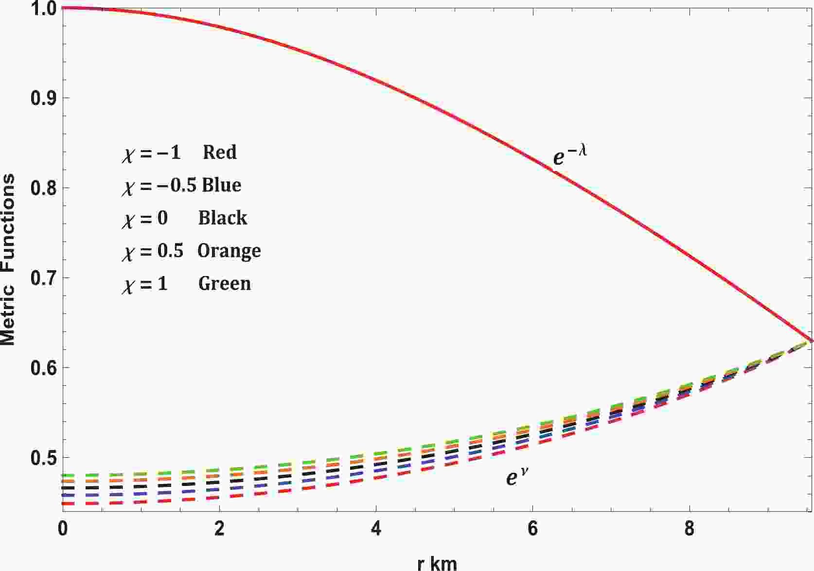
$ {\rm{erfi}}(x) $ is the usual imaginary error function. The variations in the metric functions are presented in Fig. 1.
Figure 1. (color online) Variation in metric functions with radial coordinate for Vela X-1 (
$M = 1.77 \pm 0.08 \; M_\odot,\; R = 9.56 \pm 0.08 \; {\rm km}$ ) with$b = 0.0005/{\rm km}^2$ and$c = 0.000015/{\rm km}^4$ .Plugging the metric functions into the field equations (15)-(17), one can write
$ \begin{split} \rho =& \frac{\sqrt{a {\rm e}^{b r^2+c r^4}}}{6 (\chi +2 \pi ) (\chi +4 \pi ) f_3(r) \left(a r^2 {\rm e}^{b r^2+c r^4}+1\right)^2} \Big[(\chi +3 \pi ) \\ &\times f_2(r) F\left(\frac{2 c r^2+b}{2 \sqrt{2c}}\right)+\sqrt{c} f_1(r)\Big] \end{split}, $

(29) $ \begin{split} p_r =& \frac{\sqrt{a {\rm e}^{b r^2+c r^4}}}{6 (\chi +2 \pi ) (\chi +4 \pi ) f_3(r) \left(a r^2 {\rm e}^{b r^2+c r^4}+1\right)^2} \bigg[\sqrt{c} f_4(r) \\ & + 2 \sqrt{2} a B f_5(r) {\rm e}^{b r^2+c r^4} F\left(\frac{2 c r^2+b}{2 \sqrt{2c}}\right)\bigg] \end{split}, $

(30) $ \begin{split} \Delta =& \frac{r^2 \sqrt{a {\rm e}^{b r^2+c r^4}} \left(a {\rm e}^{b r^2+c r^4}-b-2 c r^2\right)}{2 (\chi +4 \pi ) f_3(r) \left(a r^2 {\rm e}^{b r^2+c r^4}+1\right)^2} \bigg[F\left(\frac{2 c r^2+b}{2 \sqrt{2c}}\right) \\ &\times \sqrt{2} a B {\rm e}^{b r^2+c r^4} + 2 \sqrt{c} \left(A \sqrt{a {\rm e}^{b r^2+c r^4}}-B\right) \bigg] \end{split}, $

(31) $ p_t = p_r+\Delta. $

(32) where
$ \begin{split} f_1(r) =& 4 A (\chi +3 \pi ) \left(a r^2 {\rm e}^{b r^2+c r^4}+2 b r^2+4 c r^4+3\right) \\ &\times\sqrt{a {\rm e}^{b r^2+c r^4}} +B \chi \left(2 a r^2 {\rm e}^{b r^2+c r^4}+b r^2+2 c r^4+3\right), \\ f_2(r) =& 2 \sqrt{2} a B {\rm e}^{b r^2+c r^4} \left(a r^2 {\rm e}^{b r^2+c r^4}+2 b r^2+4 c r^4+3\right), \\ f_3(r) =& \sqrt{2} B \sqrt{a {\rm e}^{b r^2+c r^4}} F\left(\frac{2 c r^2+b}{2 \sqrt{2c}}\right)+2 A \sqrt{c}, \\ f_4(r) =& B \bigg[\chi \left(10 a r^2 {\rm e}^{b r^2+c r^4}-b r^2-2 c r^4+9\right)\\&+24 \pi \left(a r^2 {\rm e}^{b r^2+c r^4}+1\right)\bigg] -4 A \sqrt{a {\rm e}^{b r^2+c r^4}} \bigg[3 \pi \\ &\times \bigg(1+ a r^2 {\rm e}^{b r^2+c r^4}\bigg)-r^2 \chi \left(b-a {\rm e}^{b r^2+c r^4}+2 c r^2\right)\bigg], \\ f_5(r) =& r^2 \chi \left(b-a {\rm e}^{b r^2+c r^4}+2 c r^2\right)-3 \pi \bigg(a r^2 {\rm e}^{b r^2+c r^4} +1\bigg) . \end{split} $

The variations in density, pressures, EoS, anisotropy, and EoS parameter are displayed in Figs. 2, 3, 4, 5, and 6, respectively. The nonpolytropic nature of the EoS can be clearly seen in Fig. 4, i.e., the pressure vanishes when the surface density is greater than zero.

Figure 2. (color online) Variation in density with radial coordinate for Vela X-1 (
$M \!=\! 1.77\! \pm\! 0.08 \; M_\odot,\; R\! =\! 9.56\! \pm\! 0.08 \; {\rm km}$ ) with$b = 0.0005/{\rm km}^2$ and$c = 0.000015/{\rm km}^4$ .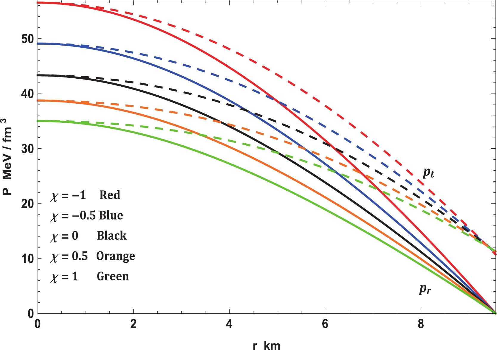
Figure 3. (color online) Variation in pressures with radial coordinate for Vela X-1 (
$M \!=\! 1.77 \pm 0.08 \; M_\odot,\; R \!=\! 9.56 \!\pm \!0.08 \; {\rm km}$ ) with$b = 0.0005/{\rm km}^2$ and$c = 0.000015/{\rm km}^4$ .
Figure 4. (color online) Equation of state for Vela X-1 (
$ M = 1.77 \pm 0.08 \; M_\odot,\; R = 9.56 \pm 0.08 \; {\rm km}$ ) with$ b = 0.0005/{\rm km}^2$ and$ c = 0.000015/{\rm km}^4$ .
Figure 5. (color online) Variation in anisotropy with radial coordinate for Vela X-1 (
$M = 1.77 \pm 0.08 \; M_\odot,\; R = 9.56 \pm 0.08 \; {\rm km}$ ) with$b = 0.0005/{\rm km}^2$ and$c = 0.000015/{\rm km}^4$ .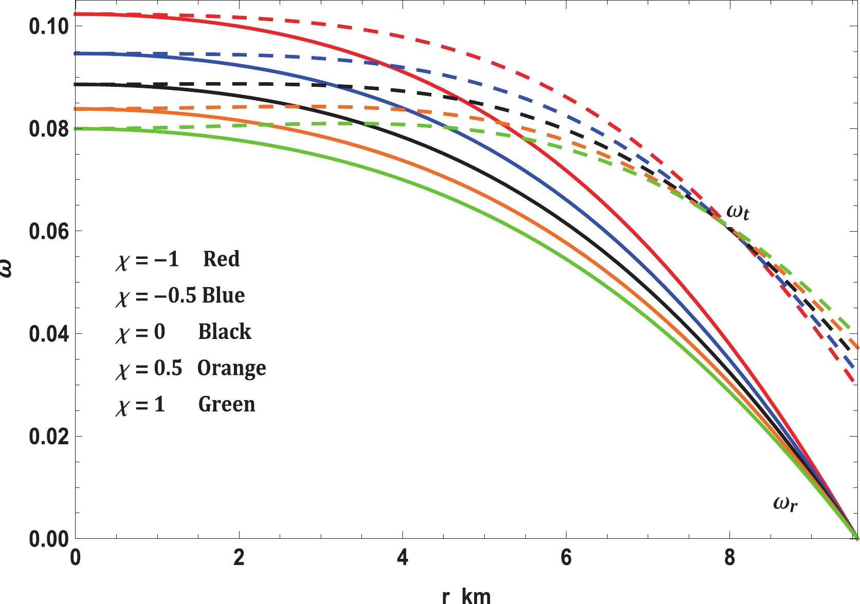
Figure 6. (color online) Variation in equation of state parameters with radial coordinate for Vela X-1 (
$M = 1.77 \pm 0.08 \; M_\odot,\; R = 9.56 \pm 0.08 \; {\rm km}$ ) with$b = 0.0005/{\rm km}^2$ and$c = 0.000015/{\rm km}^4$ . -
Any new solutions must be analyzed through various physical tests. After satisfying all the physical constraints, one can proceed further with modeling physical systems.
-
All the physical compact stars are believed to be in equilibrium states. Such equilibrium states can be tested using the equation of hydrostatic equilibrium or the modified TOV equation, which is expressed as
$ \begin{split} &-{\nu' \over 2}(\rho+p_r)-{{\rm d}p_r \over {\rm d}r}+{2\Delta \over r} \\ &\quad+{\chi \over 3(8\pi+2\chi)} {{\rm d} \over {\rm d}r} \big(3\rho-p_r-2p_t \big) = 0. \end{split} $

(33) Here, the first term is gravity (
$ F_g $ ), second term is the pressure gradient ($ F_h $ ), third term is anisotropic force ($ F_a $ ), and last term is the additional force ($ F_m $ ) in$ f(R,T)- $ gravity. The fulfillment of the modified TOV equation is presented in Fig. 7. It shows that the forces owing to gravity, pressure gradient, and$ F_m $ are the highest in$ \chi = -1 $ ; however, the anisotropic force is the lowest. This enables it to hold more mass than others for small values of$ \chi $ . As$ \chi $ increases,$ F_g,\; F_m $ , and$ F_h $ decrease although$ F_a $ increases slightly; therefore, the maximum mass that can be held by the system also reduces.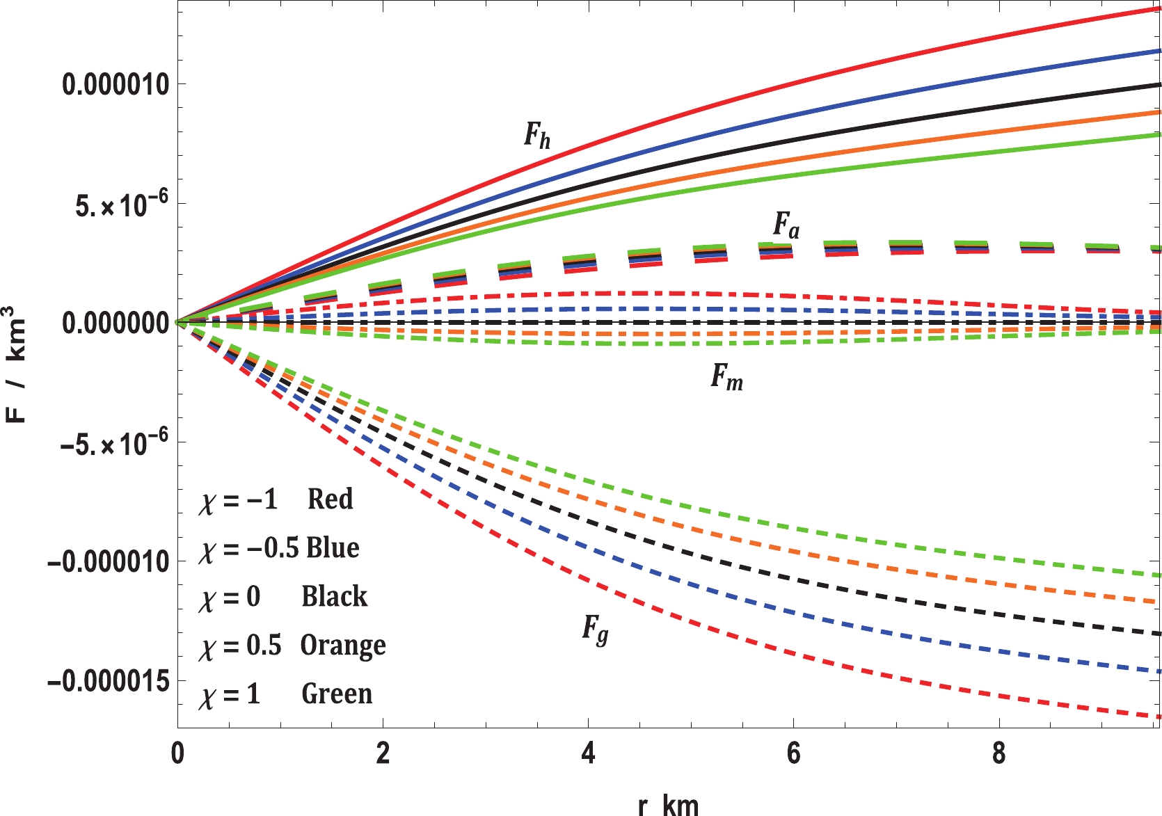
Figure 7. (color online) Variation in forces in TOV equation with radial coordinate for Vela X-1 (
$M = 1.77 \pm 0.08 \; M_\odot,\; R = 9.56 \pm 0.08 \; {\rm km}$ ) with$b = 0.0005/{\rm km}^2$ and$c = 0.000015/{\rm km}^4$ . -
We are aware of
$ f(R,T)- $ gravity as an extension of general relativity, which provides a constraint on the maximum speed limit. All the particles with nonzero rest mass travel at subluminal speeds, i.e., at less than the speed of light (causality condition). The velocity of sound in a medium must also satisfy the causality condition, and it determines the stiffness of the related EoS. Therefore, one can determine the speed of sound in a stellar medium to relate its stiffness. The most stiff EoS is Zeldovich's fluid ($ p_z = \rho_z $ ), in which sound travels exactly at the speed of light. The speed of sound can be determined as$ v_r^2 = {{\rm d}p_r \over {\rm d}\rho}\; \; ,\; \; v_t^2 = {{\rm d}p_t \over {\rm d}\rho}. $

(34) Fig. 8 presents a plot of the speed of sound with respect to the radial coordinate. It can be seen that the speed of sound is maximum for
$ \chi = -1 $ and decreases with increase in$ \chi $ . This imply that the solution leads to a stiffer EoS at small values of$ \chi $ .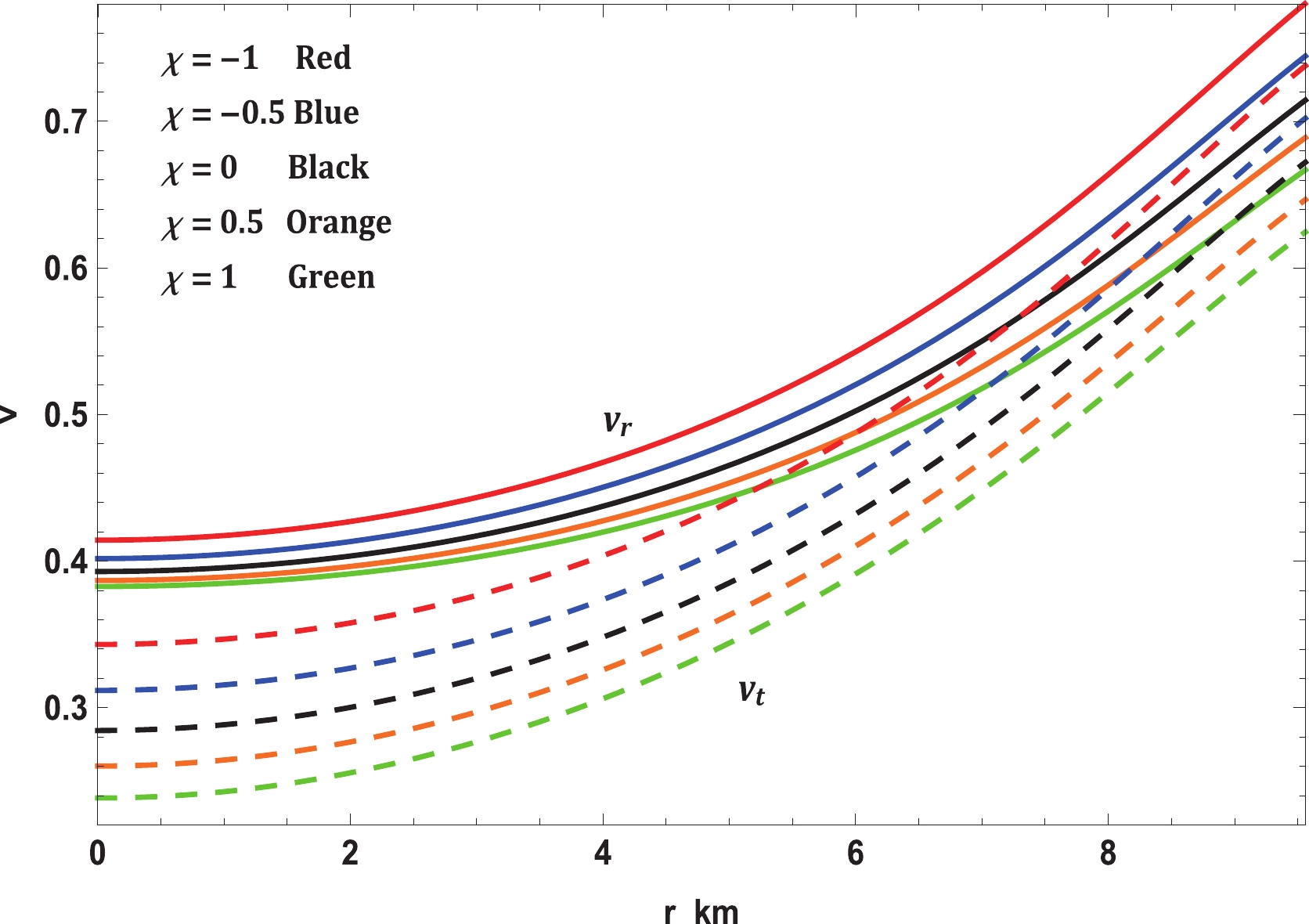
Figure 8. (color online) Variation in speed of sound with radial coordinate for Vela X-1 (
$M = 1.77 \pm 0.08 \; M_\odot,\; R = 9.56 \pm 0.08 \; {\rm km}$ ) with$b = 0.0005/{\rm km}^2$ and$c = 0.000015/{\rm km}^4$ .The speed of sound can also be related to the stability of the configuration. As per Abreu et al. [133], the stability factor can be defined as
$ v_t^2-v_r^2 $ . So long as$ v_r>v_t $ or$ -1\leqslant v_t^2 - v_r^2 \leqslant 0 $ , the system is generally considered stable, otherwise it is considered unstable. The variation in the stability factor is displayed in Fig. 9, which clearly indicates that the solution is stable.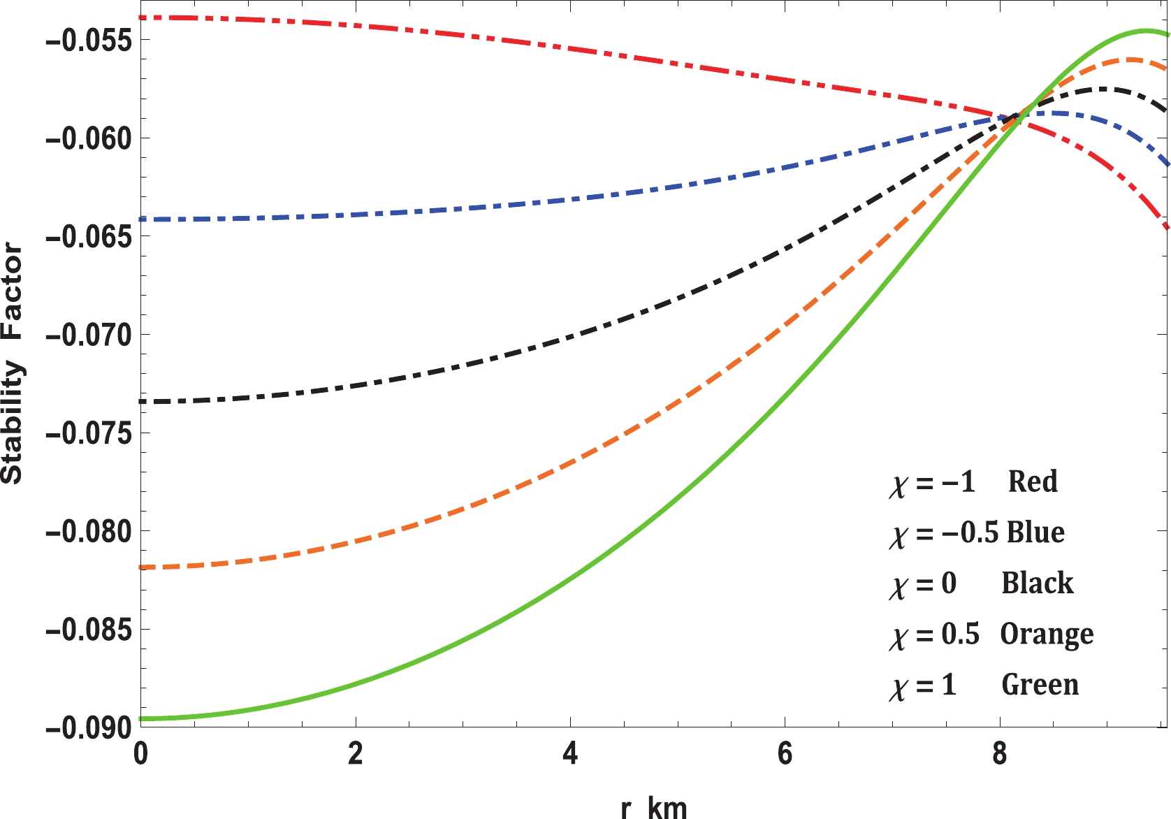
Figure 9. (color online) Variation in stability factor with radial coordinate for Vela X-1 (
$M = 1.77 \pm 0.08 \; M_\odot,\; R = 9.56 \pm 0.08 \; {\rm km}$ ) with$b = 0.0005/{\rm km}^2$ and$c = 0.000015/{\rm km}^4$ . -
Another parameter that determines the stability and stiffness of an EoS is the adiabatic index, which is defined as the ratio of specific heat at constant pressure to that at constant volume. For any fluid distribution, the adiabatic index can be determined as [134]
$ \gamma = {p_r+\rho \over p_r} v_r^2. $

(35) In polytropic cases, the pressure and density are linked by the EoS
$ p_r = K\rho^\gamma $ , and the adiabatic index$ \gamma $ is constant throughout the stellar interior. It is well-known that white dwarf stars are supported by degenerate electron pressure, and the adiabatic indexes for nonrelativistic and ultrarelativistic electrons are 5/3 and 4/3, respectively. As per Bondi's perceptions, a polytropic stellar fluid distribution is stable if$ \gamma>4/3 $ in the Newtonian limit. If$ \gamma \leqslant 1 $ , contraction is possible, and it is catastrophic if$ \gamma < 1 $ . This was extended by Chan et al. [135] to anisotropic fluids; however, it is no longer valid for anisotropic fluids, for which the stable limit of$ \gamma $ depends on the nature of anisotropy and its initial configuration. If anisotropy$ \Delta >0 $ , the stable limit will still be$ \gamma>4/3 $ ; however, if$ \Delta < 0 $ , stability is still possible even if$ \gamma < 4/3 $ . Variation in the adiabatic index is presented in Fig. 10. For various values of$ \chi $ , the central adiabatic index is accumulated around 2 and increases outward. Unlike the polytropic case, the adiabatic index is an increasing function of r and its central values decide whether the stellar configuration is stable or not.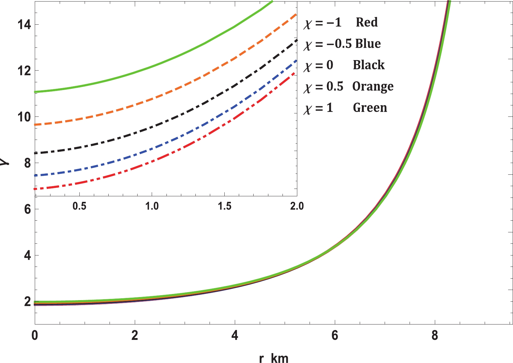
Figure 10. (color online) Variation in adiabatic index with radial coordinate and variation in mass with central density for Vela X-1 (
$M = 1.77 \pm 0.08 \; M_\odot,\; R = 9.56 \pm 0.08 \; {\rm km}$ ) with$b = 0.0005/{\rm km}^2$ and$c = 0.000015/{\rm km}^4$ . -
This criterion, originally established by Chandrasekhar, is used to analyze the stability of stellar configurations under radial perturbations [136]. Harrison et al. [137] and Zeldovich & Novikov [ 138] simplified this method later. The static stability criterion imposed the condition that if
$ \partial M / \partial \rho_c $ is greater than zero, the system is stable; otherwise, it is unstable. To verify it, we have calculated the mass as a function of$ \rho_c $ , expressed as$ M\left(\rho _c\right) = {R \over 2}\left(1-{1 \over 1+a R^2 {\rm e}^{b R^2+c R^4}}\right). $

(36) Here, a is a very complicated function of
$ \rho_c $ and, therefore, we avoid a definition. The variation of mass with respect to the central density is presented in Fig. 11, from which one can conclude that the stability is enhanced with increase in$ \chi $ . This is because the range central density is higher for saturating the mass when$ \chi = 1 $ than when$ \chi = -1 $ . This implies that the stable range of density during radial oscillation is greater for higher values of$ \chi $ . Thus, it can be concluded that this solution is stable under radial perturbations.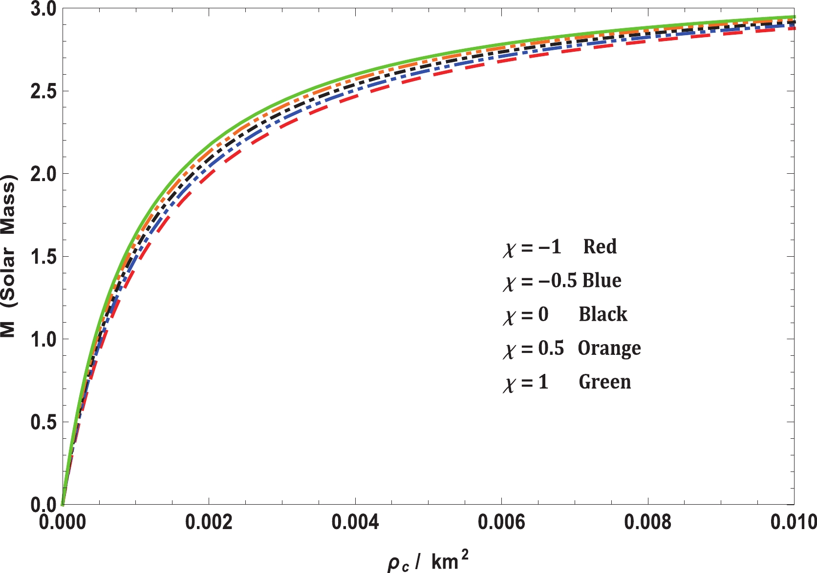
Figure 11. (color online) Variation in mass with central density for Vela X-1 (
$M = 1.77 \pm 0.08 \; M_\odot,\; R = 9.56 \pm 0.08 \; {\rm km}$ ) with$b = 0.0005/{\rm km}^2$ and$c = 0.000015/{\rm km}^4$ . -
After confirming all the stability tests, the nature of matter content, i.e., either normal (baryonic, hadronic, etc.) or exotic (dark matter, dark energy, etc.), can be identified using energy conditions. The satisfaction or violation of certain energy conditions will imply the nature of matter. These energy conditions are expressed as follows:
$ \begin{split} &{\rm{Null}}:\rho + {p_r} \geqslant 0,\;\rho + {p_t} \geqslant 0,\\ &{\rm{Weak}}:\rho + {p_r} \geqslant 0,\;\rho + {p_t} \geqslant 0,\;\rho \geqslant 0,\\ &{\rm{Strong}}:\rho + {p_r} \geqslant 0,\;\rho + {p_t} \geqslant 0,\;\rho + {p_r} + 2{p_t} \geqslant 0,\\ &{\rm{Dominant}}:\rho \geqslant |{p_r}|,\;\rho \geqslant |{p_t}|. \end{split} $

Fig. 12 indicates that all the energy conditions are satisfied by the solution and, therefore, the matter content is normal.
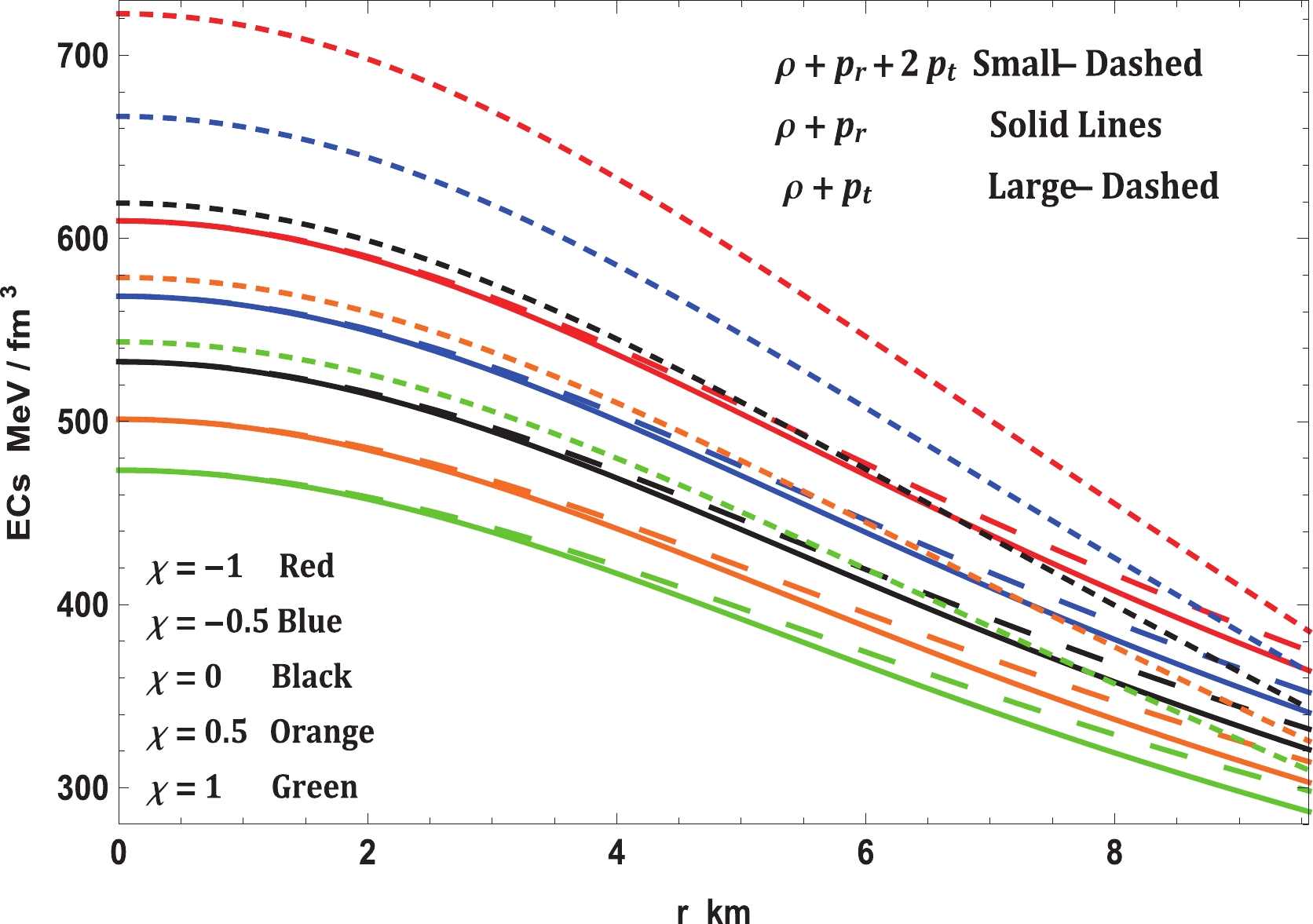
Figure 12. (color online) Variation in energy conditions with radial coordinate for Vela X-1 (
$M = 1.77 \pm 0.08 \; M_\odot,\; R = 9.56 \pm 0.08 \; {\rm km}$ ) with$b = 0.0005/{\rm km}^2$ and$c = 0.000015/{\rm km}^4$ . -
The boundary conditions ensure that the internal
$ {\cal{M}}^- $ and external space--time geometry$ {\cal{M}}^+ $ match in a smooth manner. The matching condition procedure permits the determination of the total set of constant parameters that depict the stellar model and the macrophysical observables i.e., the total mass M and the radius R of the anisotropic relativistic fluid sphere. To so do, we use the well-known Israel-Darmois junction conditions [126, 127]. As usual, we assume that the exterior space--time geometry in the form of Schwarzschild's vacuum is expressed as$ \begin{split} {\rm d}s_+^2 =& \left(1-{2m \over r}\right) {\rm d}t^2 - \left(1-{2m \over r}\right)^{-1}{\rm d}r^2 \\ & - r^2({\rm d}\theta^2 + \sin^2 \theta \; {\rm d}\phi^2). \end{split} $

(37) However, we must keep in mind that to avoid singularity, one must satisfy the condition
$ r>2m $ . Therefore, at the surface of the stellar object$ \Sigma \equiv r = R $ , the Israel-Darmois matching conditions lead to, first, the interior$ {\cal{M}}^- $ and exterior$ {\cal{M}}^+ $ manifolds expressed by Eqs. (27)-(28) and (37), respectively, induced on$ \Sigma $ as an intrinsic curvature described by the metric tensor$ g_{\mu ,\nu} $ . The continuity of the metric tensor components across the boundary$ \Sigma $ establishes the first fundamental form, which implies that$ {\rm d}s^2|_{\Sigma} = 0 $ . Second, the conditions also induce$ {\cal{M}}^- $ and$ {\cal{M}}^+ $ on$ \Sigma $ as an extrinsic geometry represented by the extrinsic curvature tensor$ K_{\mu ,\nu} $ , where$ \mu $ and$ \nu $ run over$ ( x^1, x^2, x^3 ) = (r,\theta ,\phi ) $ . The continuity of the component$ K_{r ,r} $ of the extrinsic curvature tensor across the boundary of the stellar object$ \Sigma $ infers the second fundamental form, which peruses$ p_r(r)|_{\Sigma} = 0 $ , and the continuity of the$ K_{\theta ,\theta} $ and$ K_{\phi ,\phi} $ components prompt the determination of the complete mass interior to the sphere$ m(R) = M $ . In this respect, the following remarks are appropriate. In the first situation, to acquire the complete mass governed by the anisotropic relativistic fluid sphere, at least three equivalent methods can be used: the first method is to integrate the energy density$ \rho $ over the range$ [0, R] $ , the second method is to impose the continuity of the radial components of the metric tensor$ g_{\mu ,\nu} $ across$ \Sigma $ , and the third method is based on the continuity of the angular components of the extrinsic curvature tensor$ K_{\mu ,\nu} $ . In the second situation, a vanishing radial pressure at the boundary of the stellar structure determines the radius R, i.e., the size of the stellar object; further, it avoids an indeterminate expansion of the stellar model surrounding the matter field within the region$ 0\leqslant r\leqslant R $ . Therefore, at the surface$ \Sigma \equiv r = R $ , we obtain the first fundamental form$ {\rm d}s_-^2|_{r = R} = {\rm d}s_+^2|_{r = R} $ , which explicitly reads$ {\rm e}^{-\lambda(R)} = 1-{2M \over R} = {\rm e}^{\nu(R)}. $

(38) Using Eq. (38), we obtain
$ a = \frac{2 M {\rm e}^{-R^2 \left(b+c R^2\right)}}{R^2 (R-2 M)}, $

(39) $ A = \sqrt{1-\frac{2 M}{R}}-\frac{B}{\sqrt{2 c}} \sqrt{a {\rm e}^{b R^2+c R^4}}\; F\left(\frac{2 c R^2+b}{2 \sqrt{2 c}}\right). $

(40) Generally, when modeling compact stars, the pressure at the surface should vanish, i.e., the second fundamental form
$ p_r(R) = 0 $ . This condition allows us to determine one more constant as follows:$ \begin{split} B =& 4 \sqrt{c} \sqrt{1-\frac{2 M}{R}} \sqrt{a R^2 {\rm e}^{b R^2+c R^4}} \bigg[R^2 \chi \Big(2 c R^2-a {\rm e}^{b R^2+c R^4} \\ & +b\Big)-3 \pi \left(a R^2 {\rm e}^{b R^2+c R^4}+1\right)\bigg] \bigg[\sqrt{c} R \Big\{\chi \Big(b R^2+2 c R^4 \\ &-9 -10 a R^2 {\rm e}^{b R^2 +c R^4}\Big)-24 \pi \Big(a R^2 {\rm e}^{b R^2+c R^4}+1\Big)\Big\} \\ & +2 \sqrt{2} a R {\rm e}^{b R^2+c R^4} F\left(\frac{2 c R^2+b}{2 \sqrt{2c}}\right) \Big\{3 \pi \left(a R^2 {\rm e}^{b R^2+c R^4} +1\right) \\ & -R^2 \chi \left(b-a {\rm e}^{b R^2+c R^4}+2 c R^2\right)\Big\} -{2aR \sqrt{2} \over {\rm e}^{-(b R^2+c R^4)}} \\ & F\left(\frac{2 c R^2+b}{2 \sqrt{2c}}\right) \bigg\{3 \pi \left(a R^2 {\rm e}^{-(b R^2+c R^4)}+1\right) \\ & -R^2 \chi \left(b-a {\rm e}^{-(b R^2+c R^4)}+2 c R^2\right)\bigg\}\bigg]^{-1}. \end{split} $

(41) The parameters b and c are treated as free, whereas M and R are obtained from observed evidence.
-
There are several ways of determining the stiffness of an EoS, e.g., by determining the adiabatic index, sound speed, etc. However, the sensitivity to stiffness is found to be very sharp in
$ M-R $ and$ M-I $ graphs. In fact, the$ M-I $ graph is the most effective and sensitive to the stiffness of an EoS. Fig. 14 displays the variation in mass with respect to the radius. In the preceding sections, we have already noted that the EoS is the stiffest for$ \chi = -1 $ , and as$ \chi $ increases, the stiffness reduces. Therefore, the mass that can be held by the corresponding EoS will also reduce as$ \chi $ increases. The same observations can be made from the$ M-R $ curve in Fig. 14. To compare it with the$ M-I $ curve, one must establish how to determine the moment of inertia (I). Adopting the Bejger & Haensel [ 139] formula, one can determine the value of I corresponding to a static solution. It is expressed as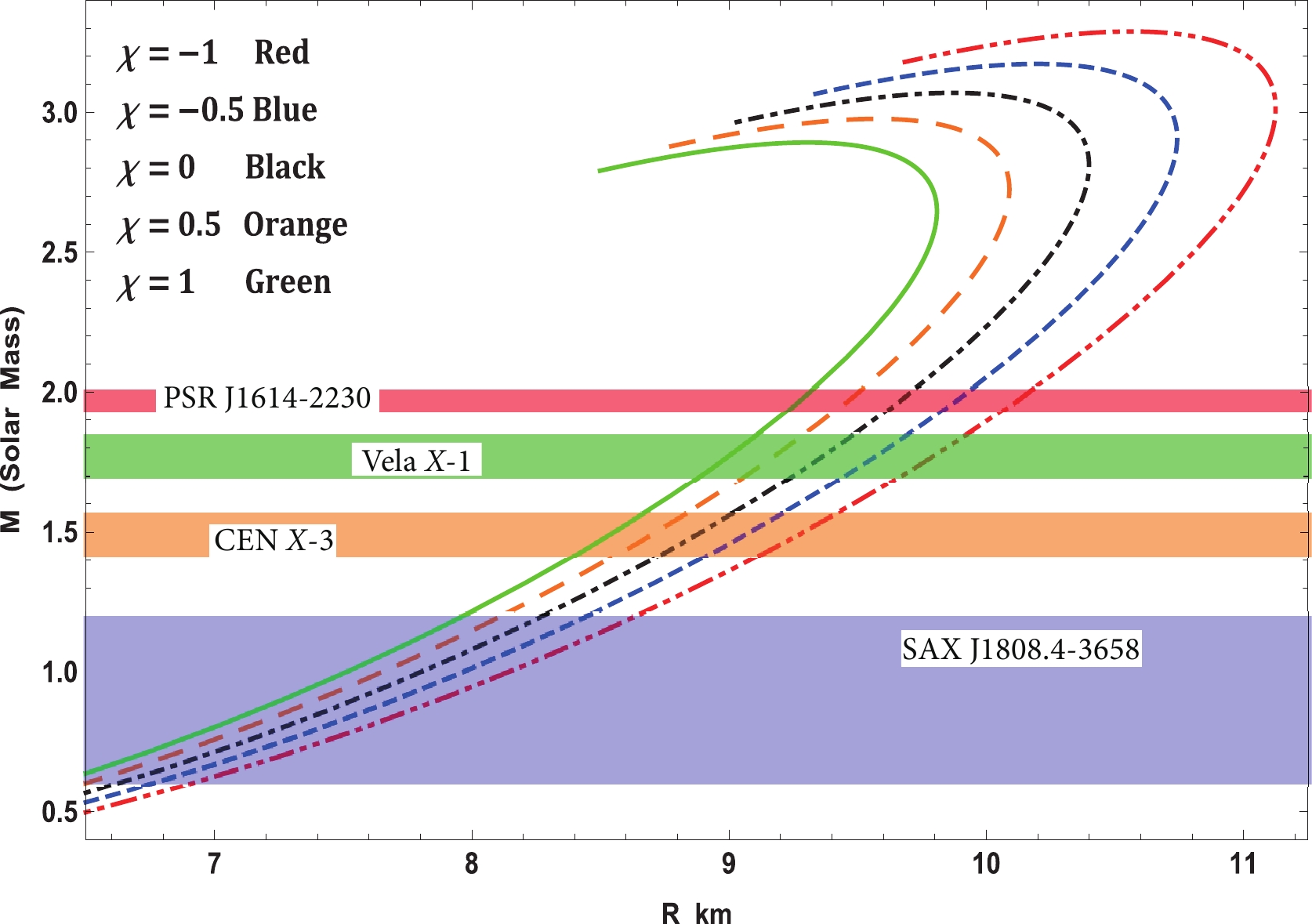
Figure 14. (color online)
$ M-R$ curve of solution.$ I = {2 \over 5} \left(1+{(M/R)\cdot {\rm km} \over M_\odot} \right)\; MR^2 . $

(42) The change in I with respect to mass is presented in Fig. 15. Again, we can verify that the EoS is most stiff for small values of
$ \chi $ . The transition at the peak of the$ M-I $ curve is sharper than that of the$ M-R $ curve, which indicates its sensitivity to the stiffness of the EoS.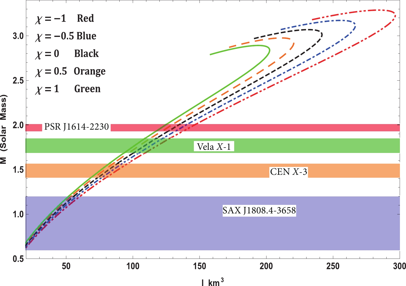
Figure 15. (color online) Variation of total mass with moment of inertia.
Further, the generated
$ M-R $ curve is also fit with observed results for a few well-known compact stars. As examples, we have matched the results obtained for PSR J1614-2230, Vela X-1, Cen X-3, and SAX J1808.4-3658. From the$ M-R $ curve fits for these compact stars, it is possible to predict the probable range of I for the abovementioned objects from the$ M-I $ curve. -
In this study, we have successfully embedded the class-one technique in the area of
$ f(R,T)- $ gravity. This procedure not only simplifies the exploration of new exact solutions within the$ f(R,T)- $ theory but also facilitates the investigation of the theory of compact stars in the same realm. The solution was analyzed through various physically stringent conditions such as the causality condition, energy conditions, satisfaction of TOV equation, stability criteria through Bondi's condition, Abreu et al. condition, and static stability criterion. As we increase the coupling constant$ \chi $ from$ -1 $ to 1, the density, pressures,$ \omega $ , speed of sound, and interior redshift increase. This increase in energy density may lead to the generation of exotic particles such as quarks, hyperons [140, 141], and kaon condensation [142], which soften the EoS. Therefore, in the$ M-R $ and$ M-I $ curves, one can see that$ M_{\rm max} $ and$ I_{\rm max} $ increase with a decrease in the coupling constant, which is a direct consequence of the stiffening of the EoS at low$ \chi $ . This outcome can also be cross-checked with the internal velocity of sound. From Fig. 8, we can see that$ v_{r/t}(\chi = -1) $ is always greater than$ v_{r/t}(\chi = 1) $ , i.e., the EoS is stiffer for the former condition as compared to the latter.Although the stiffness of the EoS is enhanced by the low coupling constant, the stability is compromised. In Fig. 10, the central value
$ \Gamma_c(\chi = 1) = 1.977 $ is greater than that at$ \Gamma_c(\chi = -1) = 1.848 $ . For$ \chi = -1 $ , the value$ \Gamma_c(\chi = -1) = 1.848 $ is comparatively closer to the Bondi limit, i.e.,$ \Gamma = 1.333 $ . Therefore,$ \chi = -1 $ is more sensitive towards radial oscillations and, hence, the stability. On the other hand, the range of central density is smaller for$ \chi = -1 $ than for$ \chi = 1 $ . This means that during radial perturbations, the range of stable density perturbation is more for$ \chi = 1 $ than for$ \chi = -1 $ , thereby enhancing its stability. Further, the solution fulfills all the energy conditions. The anisotropy decreases with decrease in the coupling parameter. This leads to the conclusion that the anisotropy in pressure reduces with increase in the stiffness of the EoS. The surface redshifts predicted form the solution in far within Ivanov's limit, i.e.,$ z_s = 3.842 $ [143].In Table 1, we have presented some of the physical parameters of four compact stars. We have also presented how the radius, central and surface densities, central pressure, and moment of inertia vary with the
$ f(R,T)- $ coupling constant. As the stiffness increases with decrease in$ \chi $ , the central and surface densities, central pressure, and radius increase while the stability is compromised. For$ -1\leqslant \chi \leqslant 1 $ , we have predicted the radii of the compact stars. All these results are accurate and in agreement with the observed values of the masses and radii. Thus, one can undoubtedly conclude that the solution might have astrophysical significance.Objects $ \chi $ 

M( $ M_\odot $ )

Predicted radius/km $ \rho_0 $ (

$ {\rm MeV}/{\rm fm}^3 $ )

$ \rho_s $ (

$ {\rm MeV}/{\rm fm}^3 $ )

$ p_0 $ (

$ {\rm MeV}/{\rm fm}^3 $ )

$ I \times 10^{44} $ (

$ g\; {\rm cm}^2 $ )

PSR J1614-2230 −1.0 1.97 $ \pm $ 0.04

10.13 621.11 376.32 72.57 18.51 −0.5 9.89 581.58 353.52 63.20 17.52 0 9.66 549.65 330.71 56.10 16.77 0.5 9.47 519.24 313.98 50.28 16.04 1.0 9.28 491.87 295.74 45.44 15.59
VELA X-1 −1.0 1.77 $ \pm $ 0.08

9.76 551.66 362.96 56.48 15.29 −0.5 9.55 518.29 339.95 49.12 14.62 0 9.34 488.38 319.24 43.36 13.94 0.5 9.15 461.91 303.13 38.76 13.56 1.0 8.99 437.75 285.87 34.85 13.01
SAX J1808.4-3658 −1.0 0.9 $ \pm $ 0.3

7.91 431.10 339.05 20.76 4.74 −0.5 7.69 403.98 317.68 18.14 4.51 0 7.54 380.96 298.78 16.12 4.34 0.5 7.42 359.60 282.34 14.50 4.17 1.0 7.26 340.69 266.73 13.19 4.00
CEN X-3 −1.0 1.49 $ \pm $ 0.08

9.29 502.10 352.97 41.72 11.24 −0.5 9.03 471.03 330.02 36.47 10.85 0 8.85 443.42 311.65 31.83 10.42 0.5 8.66 418.10 294.44 28.60 10.11 1.0 8.53 397.39 278.37 25.98 9.72 Table 1. Prediction of radius for few well-known compact stars and their corresponding central densities and pressures for various values of χ.
For the graphical test and investigation of the physical reasonable grounds of the accomplished solutions, we have selected the physical profiles of four well-known compact stellar systems, namely, PSR J1614-2230, Vela X-1, Cen X-3, and SAX J1808.4-3658. In this regard, we have assumed the radius--radius element of the metric function (
$ {\rm e}^\lambda $ ) to be in the new form$ {\rm e}^\lambda = 1+a r^2 {\rm e}^{b r^2+c r^4} $ and provided the time--time element of the metric function ($ {\rm e}^\nu $ ) as expressed explicitly in Eq. (28). Further, we exhibit the anisotropic impacts on the physical systems imposed by the$ \chi- $ coupling constant of the$ f(R, T) $ gravity theory. Thus, we have established the most significant salient features that describe the stellar system, fulfilling all the general necessities to guarantee a respectful framework.The comportment of physical amounts of time--time and radius--radius components, namely,
$ {\rm e}^\nu $ and$ {\rm e}^\lambda $ , respectively, with respect to the radial coordinate r for Vela X-1 ($ M = 1.77 \pm 0.08 \; M_\odot,\; R = 9.56 \pm 0.08 \; {\rm km} $ ) is represented in Fig. 1. This figure illustrates that both the metric functions are limited at the origin and monotonically expanding towards the point of confinement at the surface. Moreover, it may very well be seen from Eqs. (27) and (28) that$ {\rm e}^\lambda (r = 0) = 1 $ and$ {\rm e}^\nu (r = 0)\neq 0 $ , which shows that this stellar system is realistic and agreeable. Hence, Figs. 2 and 3 clearly display that all the thermodynamic observables, i.e., energy density$ \rho $ , radial pressure$ p_r $ , and transverse pressure$ p_t $ , are well-defined within the stellar structure. In this context, it is worth mentioning that all the quantities mentioned have their maximum values at the core of the stellar structure and monotonically decreasing comportment with increasing radius towards the surface. At this stage, it merits mentioning that the present stellar model shows a positive anisotropy factor$ \Delta $ ; from Fig. 3, it can be seen that when$ p_t>p_r $ ,$ \Delta >0 $ . Thus, the stellar structure is found to be a repulsive force that neutralizes the gravitational slant. This reality permits the building of a progressively compact stellar configuration. From Figs. 1, 2, and 3, we can confirm that the stellar system is absolutely devoid of physical or geometrical singularities for all chosen values of the$ \chi - $ coupling constant of the$ f(R,T)- $ gravity theory. Fig. 5 exhibits the variation in the anisotropy parameter$ \Delta $ with the radial coordinate for Vela X-1. The anisotropy vanishes at the center, and, consequently, it is defined as a positive, increasing function towards the surface of the stellar structure. In addition, Fig. 6 indicates that the values of the EoS parameters$ \omega_r = p_r /\rho $ and$ \omega_t = p_t /\rho $ are under 1, demonstrating that Zeldovich's condition is fulfilled everywhere within the stellar structure in the context of the$ f(R, T)- $ gravity theory.Further, the equilibrium study of the model for the stellar system is established using the generalized TOV equation that originates from the modified type of energy conservation equation for the energy-momentum tensor in the area of the
$ f(R,T)- $ gravity theory, as expressed in Eq. (10). In this regard, it is easy to see from Fig. 7 that the modified TOV equation permits exploration under various forces that perform on the stellar structure. In this event, the stellar structure is under the effect of four different forces, namely, gravity ($ F_g $ ), pressure gradient ($ F_h $ ), anisotropic force ($ F_a $ ), and the additional force ($ F_m $ ) in$ f(R,T)- $ gravity. The forces caused by gravity and pressure gradient and the additional force are the highest for$ \chi = -1 $ ; however, the anisotropic force is the lowest. This enables it to hold more mass than the others for small values of$ \chi $ . As$ \chi $ increases,$ F_g $ ,$ F_m $ , and$ F_h $ decrease although$ F_a $ increases slightly. Thus, the maximum mass that can be held by the system also reduces. On the other hand, we investigated the stability of realistic and compact stellar structure solutions using the causality condition and stability factor, i.e., the stability criterion through Bondi's condition and the Harrison-Zeldovich-Novikov static stability criterion corresponding to the$ \chi- $ coupling constant of$ f(R, T)- $ gravity. Fig. 8 displays the performances of the radial ($ v_r $ ) and transverse ($ v_t $ ) speeds of sound with respect to the radial coordinate r, according to these criteria, for the compact stellar configuration; it is clear that they remain within their predetermined range$ [0,1] $ throughout the stellar framework, which affirms the causality condition and, furthermore, validates the acceptability of the subsequent anisotropic solution of our stellar system. Moreover, it can be seen that the speed of sound is maximum for$ \chi = -1 $ and decreases with increase in$ \chi $ , which implies that our solution leads to a stiffer EoS at small values of the$ \chi - $ coupling constant. The solution can also be obtained for static and stable astrophysical structures, as the stability factor, which can be defined as$ v_t^{2}-v_r^{2} $ , lies between the bounds$ -1 $ to$ 0 $ for various values of the$ \chi - $ coupling parameter, displayed in Fig. 9. In addition, for a noncollapsing stellar fluid distribution, the adiabatic index should also be greater than$ 4/3 $ for$ \Delta>0 $ according to the stability criteria via Bondi’s perceptions, which can be observed clearly from Fig. 10; therefore, our stellar system is generally stable. In Fig. 11, we present the plot of the variation in mass with respect to the central density, which satisfies the Harrison-Zeldovich-Novikov static stability criterion. From this figure, one can conclude that the stability is enhanced with increase in$ \chi $ . This holds on the grounds that the range of central density is greater for saturating the mass when$ \chi = 1 $ than when$ \chi = -1 $ . This infers that the stable range of density during radial oscillation is more applicable for larger values of$ \chi $ . Thus, we can conclude that our solution is completely stable under radial perturbations. Subsequently, we investigated the profile of the thermodynamic quantities that prompt a well-behaved and positively defined energy--momentum tensor throughout the interior of the compact stellar structure, which is satisfied simultaneously by the inequalities named ECs that govern them. Hence, in Fig. 12, we present the plots of the left-hand sides of these inequalities, which verify that all the ECs are achieved at the astrophysical inside and, consequently, corroborate the physical accessibility of the compact stellar internal solution. The fulfillment of the redshift with respect to the radial coordinate r for Vela X-1 is illustrated in Fig. 13. This figure demonstrates surface redshift within typical values resulting from Ivanov’s effect, which strongly validates our compact stellar system.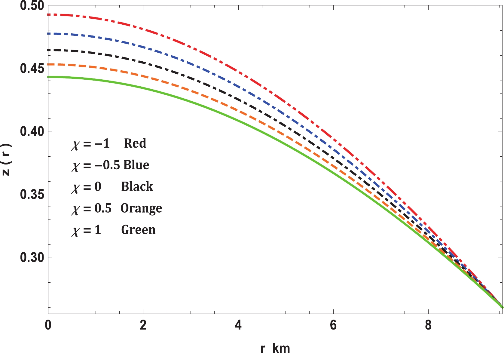
Figure 13. (color online) Variation in redshift with radial coordinate for Vela X-1 (
$M = 1.77 \pm 0.08 \; M_\odot,\; R = 9.56 \pm 0.08 \; {\rm km}$ ) with$b = 0.0005/{\rm km}^2$ and$c = 0.000015/{\rm km}^4$ .Further, we have generated
$ M-R $ curves from our solutions in the area of$ f(R, T) $ gravity theory and found a perfect fit for certain compact stellar spherical systems such as PSR J1614-2230, Vela X-1, Cen X-3, and SAX J1808.4-3658. Therefore, we have predicted the corresponding radii and their respective moment of inertia from the$ M-I $ curve by varying the coupling constant$ \chi $ as a free variable. The$ M-R $ and$ I-M $ curves are presented in Figs. 14 and 15. These curves indicate that our solution predicted the radii in good agreement with the observational data.Finally, we wish to remark that all anisotropic spherically symmetric solutions established in this study, which satisfy the well-behaved stellar interiors obtained in the area of
$ f(R, T) $ gravity theory using the embedding class-one procedure, fulfill and share all the physical and mathematical features necessary in the study of compact stellar spherical systems, leading to an understanding of the evolution of realistic compact stellar spherical systems. In this regard, the$ f(R, T) $ gravity theory is a promising principle for envisaging the existence of the compact stellar spherical systems characterized by anisotropic matter distributions, which meet the notable and tried general necessities and whose effects can be contrasted with the well-described GR.We are very grateful to the honorable referees and the editor for their relevant suggestions that have considerably improved our work in terms of the quality of research and presentation.
Exploring physical properties of compact stars in
${ f(R,T)}$
-gravity: An embedding approach
- Received Date: 2020-04-09
- Available Online: 2020-10-01
Abstract: Solving field equations exactly in


 DownLoad: