


 Abstract
 HTML
HTML Reference
 Related
 PDF
PDF


-
Dark energy, the source of the late-time accelerating expansion, has been considerably studied since the observations of type Ia supernovae. For example, in Ref. [1], the authors constructed the type Ia supernova spectrum by training an artificial neural network; in Ref. [2], bulk viscosity of dark energy is taken into account to alleviate the age problem of the universe; and in Ref. [3], dark energy is investigated in the brane world scenario to avoid the big rip ending of the universe. For reviews on dark energy see Refs. [4] and [5]. It has been shown that more than two-thirds of the energy density in the universe is completely unknown, after which the dark energy is named. The equation of state of dark energy is known to be nearly
$ w\sim-1 $ at present [6]. The gravitational force generated by the dark energy is of the repulsive kind; however, on the Earth, no one has observed such anti-gravity force in a lab.The vacuum energy from the quantum field theory or the cosmological constant from general relativity can be considered as a kind of dark energy, for its equation of state
$ w = -1 $ . However, observations have not confirmed$ w = -1 $ , and it actually deviates from$ -1 $ slightly [6], which implies that a dynamical dark energy with varying$ w $ may be more consistent with the observations. Quintessence is a kind of dynamical dark energy model, in which a scalar field, minimally coupled to gravity, drives the universe to accelerate. Recently, a scalar field that was once used to make the universe inflate in the early time [7-11] with a pole in its kinetic term is proposed as a new kind of dark energy model [12], which is called the pole dark energy model. In this model, the original field that is non-minimally coupled to the gravity does not need a very unnatural flat potential. The transformation that converts the original field with non-canonical kinetic term into an altered one with canonical kinetic term could make the potential of the new field much more flat. Then the universe will be accelerated by this flat potential energy. Thus, the pole dark energy model may fundamentally explain why the potential is so flat in the standard quintessence dark energy model.We generalize the pole dark energy model and propose a multi-pole one, in which the kinetic term may have multiple poles. Poles can come from the super-gravity theory due to the non-minimal coupling to the gravitational field or the geometric properties of the Kähler manifold [13, 14]. The k-essence model [15] is a dark energy model with non-canonical kinetic terms. Here, we treat it phenomenologically similar to what has been done in Ref. [12]. We find that the poles can place some restrictions on the values of the original scalar field, which implies that the original scalar field does not need to change considerably when its corresponding transformed field with canonical kinetic term changes significantly. The later time evolution of the universe is obtained explicitly for the two pole model, while the dynamical analysis is performed for the multiple pole model. We find that it does have a stable solution, which corresponds to the universe dominated by the potential energy of the scalar field.
In Sec. 2, we introduce the multi-pole dark energy model. The relation between the original scalar field that has two poles in its kinetic term and the transformed canonical one will be shown, and the properties of the transformed potential will also be presented. The cosmological evolution driven by the two pole model will be given in Sec. 3. For a general multi-pole dark energy, we will perform the dynamical analysis in Sec. 4. In Sec. 5 discussions and conclusions will be presented.
-
In general, the Lagrangian for a scalar field with poles in the kinetic term can be written as
$ \begin{split} {\cal{L}} = -\frac{1}{2}\frac{k^2}{f^2(\sigma)}(\partial\sigma)^2 - V(\sigma)\,, \end{split} $

(1) where
$ V(\sigma) $ is the potential, and$ f(\sigma) $ is some function of the scalar field. Function$ f $ may have multiple zero points by construction. The parameter$ k $ can be positive or negative. Without loss of generality,$ k $ will be taken as$ \pm1 $ in the numerical calculations. Poles can come from the super-gravity theory owing to the non-minimal coupling to the gravitational field or the geometric properties of the Kähler manifold. In the pole dark energy model in Ref. [12], function$ f $ is taken as a power law:$ f(\sigma) = \sigma^{p/2} $ with positive$ p $ , and the pole resides at only one point$ \sigma = 0 $ with residue$ k^2 $ and order$ p $ . In the Brans-Dicke theory, the pole corresponds to the case of$ p<2 $ in the pole dark energy model, and in such a case, it steepens the transformed potential instead of making it flat. Hence, the parameter region with$ p<2 $ is not very interesting to be considered in the pole dark energy model [12]. -
After performing the transformation
$ {\rm d}\phi = k{\rm d}\sigma/f(\sigma) $ , which indicates that the case of$ k<0 $ is equivalent to changing the overall sign of the$ f $ function while keeping$ k $ positive, the non-canonical kinetic term of$ \sigma $ is transformed to the canonical form for the scalar field$ \phi $ :$ \begin{split} {\cal{L}} = -\frac{1}{2}(\partial \phi)^2 - V(\sigma(\phi))\,. \end{split} $

(2) The function
$ f $ can phenomenologically take the following form:$ \begin{array}{l} f(\sigma) = \sigma^{p/2}(1 -\beta\sigma^q) \,, \end{array} $

(3) which residues at
$ \sigma = 0 $ and$ \sigma = \beta^{-1/q} $ with parameters$ q>1,\; \beta>0 $ in the unit of$ 8\pi G = 1 $ . In the case of$ p\neq 2 $ , we have$ \begin{split} \phi = -\frac{2}{p-2} \sigma^{1-\frac{p}{2}} \, _2F_1\left(1,\frac{1-\frac{p}{2}}{q};\frac{1-\frac{p}{2}+q}{q};\beta \sigma^q\right) \,, \end{split} $

(4) where
$ _2F_1 $ is the hypergeometric function. For$ p = 2 $ we can get a more simple explicit relation between$ \phi $ and$ \sigma $ :$ \phi = \frac{k}{q}\ln\bigg(\frac{\sigma^q}{1-\beta\sigma^q} \bigg)\,, $

(5) $ \sigma = \left(\frac{1}{{\rm e}^{-q\phi/k}+\beta } \right)^{1/q} \,. $

(6) When
$ k>0,\; \beta = 0 $ , we have$ f = \sigma $ from Eq. (3), which is just the pole dark energy model in Ref. [12] with$ p = 2 $ there. This model is often used for inflation. When$ k<0 $ ,$ f\sim \beta \sigma^{q+1} $ for large$ \sigma $ , which coincides with the pole dark energy model when$ p = 2{q+1} $ . Function$ f $ can be also written in terms of$ \phi $ :$ \begin{array}{l} f = {\rm e}^{\phi/k}\bigg( 1+\beta {\rm e}^{q\phi/k}\bigg)^{-1-\frac{1}{q}} \,. \end{array} $

(7) We will consider the branch
$ 0<\sigma<\beta^{-1/q} $ , which corresponds to$ \phi\in(-\infty, \infty) $ . By contrast,$ \sigma $ is considered in the branch of$ \sigma>0 $ in the pole dark energy model. It shows that the second pole puts a constraint on the$ \sigma $ field. When the parameter$ q $ is chosen to be$ q<-1 $ , it takes the branch$ \sigma>\beta^{-1/q} $ correspondingly, see Eq. (6). Therefore, when two poles are very close to each other, such as for a very large$ \beta $ in the two pole model, one can take another branch by setting suitable values of the parameters, such as$ q<-1 $ and the result will remain unchanged.In the case of power law potential, we have
$ \begin{array}{l} V \sim \sigma^n \,, \rightarrow V \sim (\beta + {\rm e}^{-q\phi/k})^{-n/q} \,. \end{array} $

(8) For
$ k>0 $ , when$ \phi $ goes to infinity, the potential becomes$ \begin{split} V|_{\phi\rightarrow\infty} \sim \beta^{-\frac{n}{q}}\left(1-\frac{n}{q\beta}{\rm e}^{-q\phi/k}\right)\,, \end{split} $

(9) which is basically an uplifted exponential potential. Otherwise, when
$ \phi $ goes to minus infinity, the potential becomes$ V|_{\phi\rightarrow-\infty}\sim {\rm e}^{n\phi/k} $ . For$ k<0 $ , the limits are exchanged. Note that after transforming to the canonical form, we get a flat potential for the transformed new scalar field$ \phi $ even if the original field$ \sigma $ has a steep one. The first derivative of the potential with respect to$ \phi $ is given by:$ \begin{split} \frac{V_\phi}{V} \equiv \frac{{\rm d}V/{\rm d}\phi}{V} = \frac{n}{k} \frac{ {\rm e}^{-q\phi/ k}}{\beta + {\rm e}^{-q\phi/k}} \,. \end{split} $

(10) When
$ \beta = 0 $ ,$ V_\phi/V $ is a constant. However, in the case of$ \beta \neq 0 $ ,$ V_\phi/V \sim {\rm e}^{-q\phi/k} $ . For$ k>0 $ , when$ \phi $ is large,$ V_\phi/V\ll 1 $ , which indicates that the potential has a flat plateau at that moment.In the case of a dilaton potential, we have
$ \begin{array}{l} V\sim {\rm e}^{-\alpha\sigma}\,,\rightarrow V\sim {\rm e}^{-\alpha (\beta + {\rm e}^{-q\phi/k})^{-1/q} }\,, \end{array} $

(11) which gives a super-exponential behavior as that in Ref. [12]. And
$ V_\phi/V $ is$ \begin{split} \frac{V_\phi}{V} = \frac{\alpha}{k} \frac{ {\rm e}^{-q\phi/k}}{\beta + {\rm e}^{-q\phi/k}} \frac{1}{(\beta + {\rm e}^{-q\phi/k})^{1/q}}\,. \end{split} $

(12) When
$ \beta = 0 $ ,$ V_\phi/V \sim {\rm e}^{\phi/k} $ , and while$ \beta\neq 0 $ and$ k>0 $ ,$ V_\phi/V \sim {\rm e}^{-q\phi/k} $ , which also gives a flat plateau-like potential.In fact, for a general potential
$ V(\sigma) $ , we have$ \begin{split} \frac{V_\phi}{V} = \frac{V_\sigma}{V}\frac{f}{k} = \frac{V_\sigma}{V} \frac{{\rm e}^{-q\phi/k}}{(\beta + {\rm e}^{-q\phi/k})^{1/q+1}}\,. \end{split} $

(13) When
$ \phi\rightarrow \infty $ ,$ \sigma $ approaches its second residue$ \sigma\rightarrow \beta^{-1/q} $ from Eq. (6). Then$ V_\sigma/V $ becomes a constant, and$ V_\phi/V\sim {\rm e}^{-q\phi/k} $ . Thus, the second pole in the kinetic term of$ \sigma $ can be significantly helpful for achieving a flat plateau-like potential without fine-tuning any parameters. -
When the function
$ f(\sigma) $ in the kinetic term of$ \sigma $ is taken as a general function instead of a simple one like Eq. (3), the analytical formula for$ V(\phi) $ cannot be always obtained; therefore, we will perform the dynamical analysis for this general case in Sec. 4. Note that we always consider a branch of$ \sigma $ that does not cross the residue points. For example, in the previous section$ \sigma\in(0,\beta^{-1/q}) $ . This implies that the zeros of$ f(\sigma) $ will place some restrictions on the values of$ \sigma $ . The change of$ \sigma $ field is then relatively small during the evolution, even when there is a big change in the$ \phi $ field. With the help of poles in the kinetic term of$ \sigma $ or zero points of the function$ f(\sigma) $ , we can get a flat plateau-like potential easily, since$ V_\phi/V\rightarrow 0 $ when$ f $ approaches any one of its zero points, see Eq. (13). -
The late-time evolution of a flat universe is determined by the Friedmann equation:
$ \begin{split} H^2 = \frac{1}{3M_p^2}\left(\rho_m + \frac{1}{2}\dot\phi^2 + V(\phi)\right) \,, \end{split} $

(14) which includes the dark matter and dark energy components. Here,
$ M_p^2 = 1/8\pi G $ is the reduced Planck mass, and$ M_p = 1 $ in the unit of$ 8\pi G = 1 $ . The dot over$ \phi $ denotes the derivatives with respect to time, and$ \rho_m $ is the energy density of dark matter. The equation of motion for the$ \phi $ field is given by$ \ddot \phi + 3H\dot \phi +\frac{{\rm d}V}{{\rm d}\phi} = 0\,. $

(15) We also have the dynamic equation:
$ \dot H = -\frac{1}{2} (\rho_m + \dot\phi^2)\,. $

(16) Let
$ x = \ln a $ and introduce the following field and potential:$ \psi = \frac{\phi}{M_p}\,, \quad U = \frac{V}{3H_0^2M_p^2}\,, $

(17) where we have recovered the unit to see that both
$ \psi $ and$ U $ are dimensionless and$ H_0 $ is the present value of the Hubble parameter. Then, the Friedmann equation becomes$ E^2 \left( 1-\frac{1}{6}\psi'^2\right) = \Omega_{m0} {\rm e}^{-3x} + U \,, $

(18) where the prime denotes the derivatives with respect to
$ x $ and$ \Omega_{m0}\equiv \frac{\rho_{m0}}{3H_0^2} $ ,$ E\equiv H/H_0 $ . Eq. (16) becomes$ EE' = -\frac{3}{2}\Omega_{m0} {\rm e}^{-3x} + \frac{1}{2} E^2\psi'^2\,. $

(19) After a straightforward calculation, the equation of motion for
$ \psi $ could be written as$ \begin{split} \bigg(\Omega_{m0} {\rm e}^{-3x} + U\bigg)\left( \psi'' + \frac{1}{2} \psi'^3 +3\psi'\right) +3\left( 1-\frac{1}{6}\psi'^2\right)\left(\frac{{\rm d}U}{{\rm d}\psi}-\frac{1}{2}\Omega_{m0} {\rm e}^{-3x}\psi'\right) = 0\,. \end{split} $

(20) The equation of state is given by
$ \begin{split} w = \frac{\dot\phi^2/2-V}{\dot\phi^2/2+V} = -1+2\left[1+\frac{U\left( 6-\psi'^2\right)}{(\Omega_{m0} {\rm e}^{-3x} + U)\psi'^2}\right]^{-1} \,. \end{split} $

(21) It is clear that when the
$ \psi $ field's kinetic energy is mu-ch smaller than its potential,$ w\sim -1 $ . The evolution of the field$ \psi $ can be obtained by numerically solving Eq. (20).For
$ V = m^2\sigma^2/2 $ with,$ U = U_0(\beta + {\rm e}^{-q\psi/k})^{-2/q}\,,\quad U_0 = \frac{m^2}{6H_0^2}\,, $

(22) and
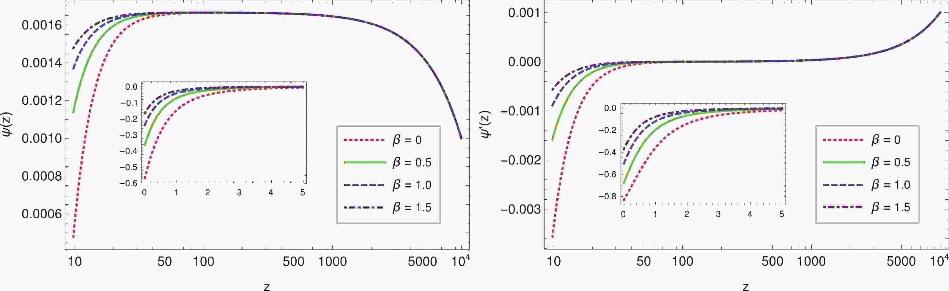
$ q = 2 $ we solved Eq. (20) and plotted the evolution of$ \psi $ as the redshift$ z = 1/a-1 $ in Fig. 1. One can always make$ k^2 = 1 $ by redefining$ \sigma $ . Therefore, without losing generality, we set$ k = 1 $ in the numerical calculations. Note that$ k = -1 $ is equivalent to changing the overall sign of the function$ f $ while keeping$ k = 1 $ , see Eq. (3). In other words, when$ k = -1 $ , we can redefine$ \psi\rightarrow -\psi $ , then$ U $ will neither change in Eq. (22) nor will Eq. (15).
Figure 1. (color online) The evolution of
$ \psi $ and$ \psi' $ with power law potential as a function of redshift$ z $ with the same initial conditions and with$ \Omega_{m0} = 0.3,\;q = 2,\;\alpha = 1 $ and different$ \beta $ values.As can be seen in Fig. 1,
$ \psi $ increases in the early time and decreases at present$ z\rightarrow 0 $ . It shows that large value of$ \beta $ could slow down the decreasing process of$ \psi $ , and suppress the increase in the kinetic momentum energy$ \sim \psi'^2 $ . This indicates that with the help of$ \beta $ , the potential energy will be the main part of the energy of$ \psi $ ; therefore, its equation of state will be$ w\rightarrow-1 $ , see Fig. 2. It should be noticed that there is two to three orders of magnitude difference between the main coordinate values of the$ \psi(z) $ axis in the main panels and those in the inset for small$ z $ in Fig. 1 (and also in Fig. 5).
Figure 2. (color online) For power law potential, the evolution of the equation of state
$ w $ and its running$ w' $ as the function of redshift$ z $ with$ \Omega_{m0} = 0.3,\;q = 2,\;n = 2 $ and different$ \beta $ values.
Figure 5. (color online) The evolution of
$ \psi $ and$ \psi' $ with dilaton potential as the function of redshift$ z $ with the same initial conditions and with$ \Omega_{m0} = 0.3,\;q = 2,\;\alpha = 1 $ and different$ \beta $ values.
Figure 6. (color online) For dilaton potential, the evolution of the equation of state
$ w $ and its running$ w' $ as a function of redshift$ z $ with$ \Omega_{m0}=0.3,\;q=2,\;\alpha=1 $ and different$ \beta $ values.The evolution of the equation of state
$ w $ and its running$ w' $ are plotted in Fig. 2. We also plot their phase space in Fig. 3. It is evident that the large values of$ \beta $ could indeed make the model much more suitable to describe the present accelerating universe. Further, the running of$ w $ almost vanishes ($ w'\sim 0 $ ) at present when$ \beta $ is large. The ratio of the Hubble parameter with$ \beta\neq 0 $ to that with$ \beta = 0 $ is plotted in Fig. 4, from which one can see that the Hubble parameters with different$ \beta $ values have slight differences at the low redshifts. The deceleration parameter$ q = -\ddot a/(aH^2) $ is also plotted in Fig. 4, and it shows that large values of$ \beta $ could indeed drive the cosmic acceleration much more easily.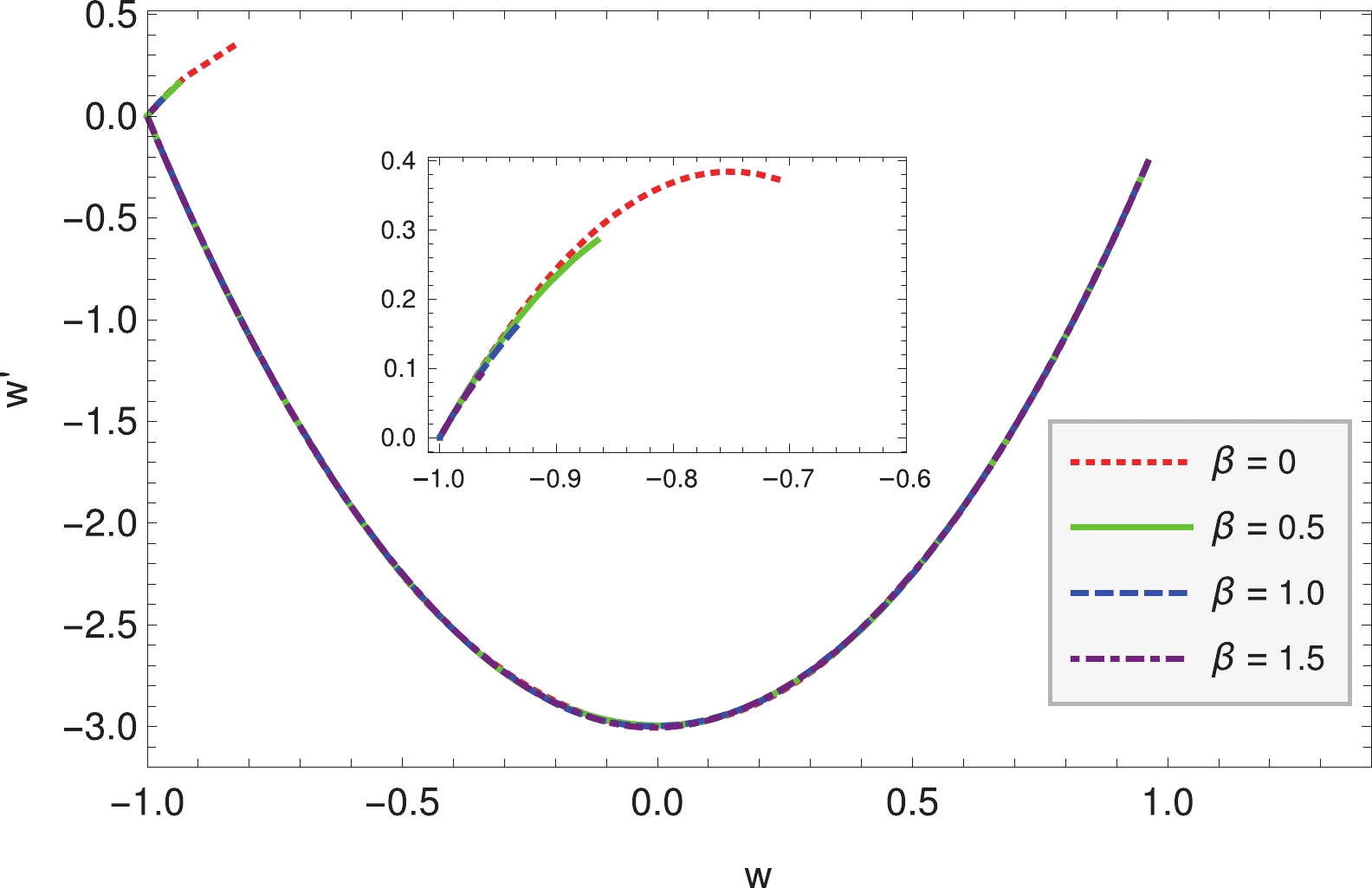
Figure 3. (color online) For power law potential, the dynamics of
$ w-w' $ phase space with$ \Omega_{m0} = 0.3,\;q = 2,\;n = 2 $ and different$ \beta $ values.
Figure 4. (color online) For power law potential, the ratio of the Hubble parameter with
$ \beta\neq 0 $ to that with$ \beta = 0 $ and the deceleration parameter$ q(z) $ as a function of redshift$ z $ with$ \Omega_{m0} = 0.3,\;q = 2,\;n = 2 $ and different$ \beta $ values.Now we take the potential as
$ V = V_0{\rm e}^{-\alpha \sigma} $ , or$ \begin{split} U = U_0{\rm e}^{-\alpha (\beta + {\rm e}^{-q\psi/k})^{-1/q} } \,,\quad U_0 = \frac{V_0}{6H_0^2}, \end{split} $

(23) to solve Eq. (20) numerically. The evolution of
$ \psi $ and$ w $ and their derivatives are plotted in Figs. 5-7, while the ratio of the Hubble parameter with$ \beta\neq 0 $ to that with$ \beta = 0 $ and the deceleration parameter are also plotted in Fig. 8. The role of$ \beta $ is almost the same as that in the model with power law potential.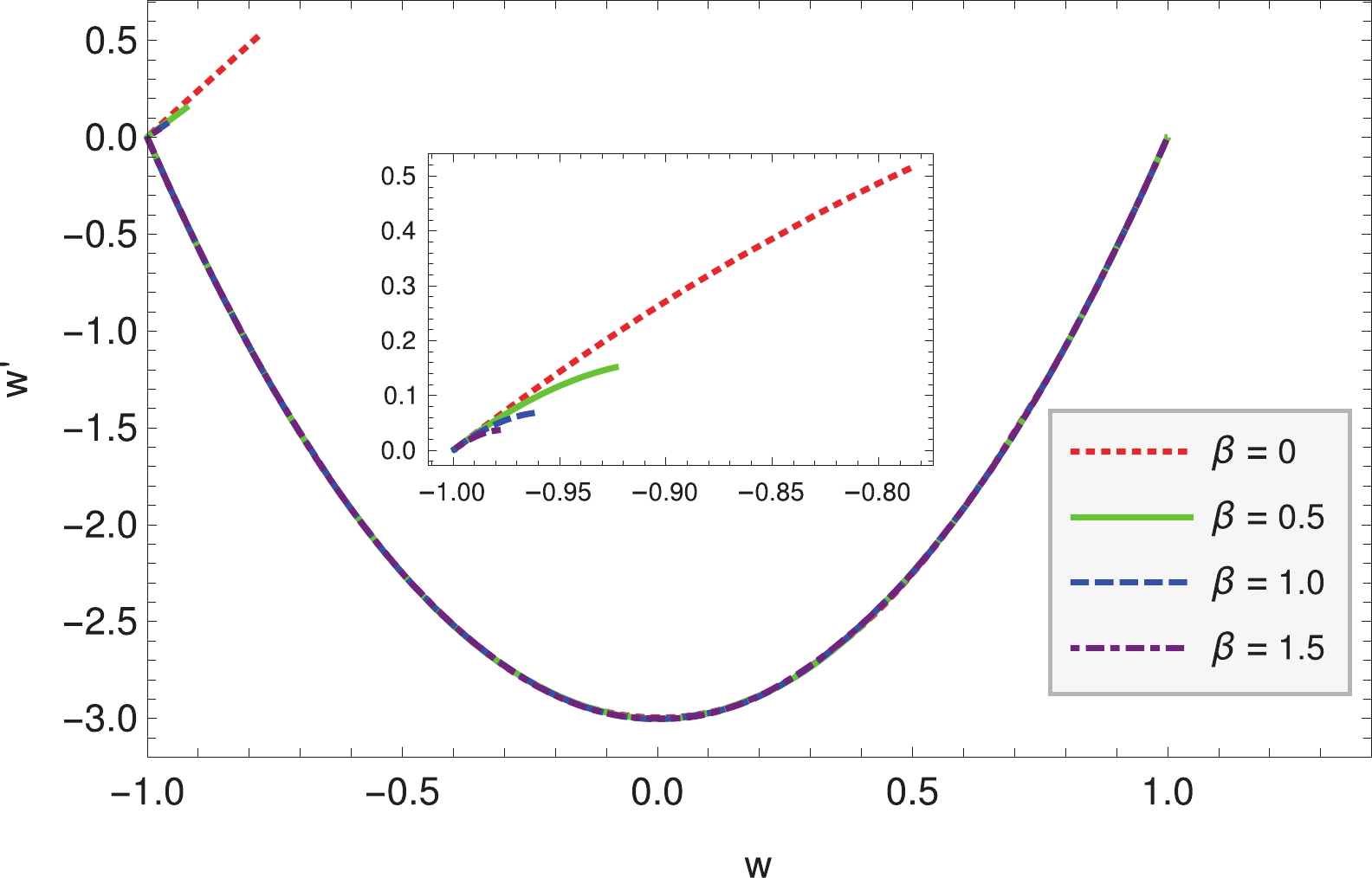
Figure 7. (color online) For dilaton potential, the dynamics of
$ w-w' $ phase space with$ \Omega_{m0} = 0.3,\;q = 2,\;\alpha = 1 $ and different$ \beta $ values.
Figure 8. (color online) For dilaton potential, the ratio of the Hubble parameter with
$ \beta\neq 0 $ to that with$ \beta = 0 $ and the deceleration parameter$ q(z) $ as a function of redshift$ z $ with$ \Omega_{m0} = 0.3,\;q = 2,\;\alpha = 1 $ and different$ \beta $ values. -
Dynamical analysis is an effective method to reveal the novel phenomena arising from nonlinear equations without solving them. It can produce good numerical estimates of the parameters connected with the general features such as stability. This method has already been used for analyzing the evolution of the universe; see Refs. [16-17].
In this section, we will treat the
$ f(\sigma) $ as a general function, which may have multiple zero points, and perform the dynamical analysis on the whole system of equations. -
From Eq. (15) and using
$ {\rm d}\phi = k{\rm d}\sigma/f $ , we have$ \begin{split} \ddot \sigma-\frac{{\rm d}f}{f{\rm d}\sigma}\dot \sigma^2+3H\dot \sigma + \frac{{\rm d}V}{{\rm d}\sigma}\frac{f^2}{k^2} = 0\,. \end{split} $

(24) After defining the dimensionless variables in the units of
$ 8\pi G = 1 $ :$ X = \frac{k\dot\sigma}{\sqrt{6}fH}\,,\quad Y = \frac{\sqrt{V}}{\sqrt{3} H} \,,\quad \lambda = \frac{f}{k}\frac{V_\sigma}{V}\,, $

(25) with potential
$ V_\sigma = {\rm d}V/{\rm d}\sigma $ , we have the constraint arising from the Friedmann equation$ 1 = \Omega_m + X^2+Y^2 \,, \quad \Omega_m = \frac{\rho_m}{3H^2}\,, $

(26) therefore, the whole dynamical system is given by
$\frac{{\rm d}X}{{\rm d}x} = -3X- \sqrt{\frac{3}{2}} \lambda Y^2+ \frac{3}{2}X(1+X^2-Y^2) \,, $

(27) $ \frac{{\rm d}Y}{{\rm d}x} = Y\left[ \sqrt{\frac{3}{2}} \lambda X +\frac{3}{2}(1+X^2-Y^2)\right]\,, $

(28) $ \frac{{\rm d}\lambda}{{\rm d}x} = \sqrt{6}X\lambda \left( \Gamma -\lambda \right)\,, $

(29) where
$ \Gamma \equiv \frac{f_\sigma}{k} + \lambda \frac{VV_{\sigma\sigma}}{ V_\sigma^2}\,, $

(30) with the convention
$ f_\sigma = {\rm d}f/{\rm d}\sigma,\; V_{\sigma\sigma} = {\rm d}^2V/{\rm d}\sigma^2 $ . The equation of state can also be written in terms of$ X,\;Y $ :$ w = \frac{X^2-Y^2}{X^2+Y^2}\,. $

(31) Generally, the system (27)-(29) is not a strictly autonomous system, but in some cases it is indeed an autonomous system. For example, when
$ \Gamma = \lambda $ . In this case, it implies$ \frac{{\rm d}f/{\rm d}\sigma}{f} = \frac{{\rm d}V/{\rm d}\sigma}{V}-\frac{{\rm d}^2V/{\rm d}\sigma^2}{{\rm d}V/{\rm d}\sigma}\,. $

(32) After integrating the above equation, we have
$ f\dfrac{{\rm d}V}{{\rm d}\sigma}\sim V $ up to some integration constant. By using the transformation$ \phi = \int \frac{{\rm d}\sigma}{f} \sim \int \frac{{\rm d}V}{V{\rm d}\sigma}{\rm d}\sigma = \ln V\,, $

(33) we then get an exponential potential for
$ \phi $ . Taking$ V = m^2\sigma^2/2 $ , we get$ f\sim \sigma $ , which corresponds to the$ \beta = 0 $ case in Eq. (22). When$ \Gamma = \lambda $ , it shows$ \lambda = \lambda_c $ is a constant due to Eq. (29). The dynamical system then reduces to a$ 2- $ dimensional one. When$ \lambda_c\neq 0 $ , there are five critical points ($ X_c,Y_c $ )$ (0,0)\,, (1,0)\,,(-1,0) \,,\left(-\frac{\lambda_c}{\sqrt{6}},\sqrt{1-\frac{\lambda_c^2}{6}}\right)\,,\left(-\sqrt{\frac{3}{2}}\frac{1}{\lambda_c},\sqrt{\frac{3}{2}}\frac{1}{\lambda_c}\right)\,. $

(34) These critical points are the same as those for a quintessence model, and their stabilities have already been investigated in the literature, see Ref. [5] and references therein.
When
$ \Gamma\neq \lambda $ , Eqs. (27)-(29) do not form an autonomous system. By construction, the$ f $ function has multiple zero points. When the system approaches one of the zero points,$ \lambda $ will nearly vanish due to the definition of$ \lambda\sim f $ in Eq. (25). The derivative of$ \Gamma $ with respect to$ x $ is given by$ \frac{{\rm d}\Gamma}{{\rm d}x} = \frac{f_{\sigma\sigma}f}{k^2}\sqrt{6}X + \frac{{\rm d}\lambda}{{\rm d}x} \frac{VV_{\sigma\sigma}}{ V_\sigma^2} + \lambda \frac{{\rm d}}{{\rm d}x}\left( \frac{VV_{\sigma\sigma}}{ V_\sigma^2}\right)\,. $

(35) When
$ f\rightarrow0 $ , we have$ \lambda\sim 0 $ ,$ {\rm d}\lambda/{\rm d}x\sim 0 $ due to Eq. (29) and correspondingly$ {\rm d}\Gamma/{\rm d}x\sim 0 $ due to the above equation.By introducing the following variables:
$ \Gamma_{A(1)} = \frac{f^{\sigma} }{k}, $

(36) $ \Gamma_{A(n)} = \frac{f^{(n)} f^{n-1}}{f_\sigma^{n}} \,, \quad \Gamma_{B(n)} = \frac{V^{(n)} V^{n-1}}{V_\sigma^{n}} \,, \quad n\geqslant 2\,, $

(37) where
$ f^{(n)} \equiv {\rm d}^nf/{\rm d}\sigma^n $ and$ V^{(n)} \equiv {\rm d}^nV/{\rm d}\sigma^n $ , we can rewrite$ \Gamma $ as a sum of two parts:$ \begin{array}{l} \Gamma = \Gamma_{A(1)} + \lambda\Gamma_{B(2)} \,; \end{array} $

(38) therefore, the dynamical equations for these variables are given by
$ \begin{split} \frac{{\rm d}\Gamma_{A(1)}}{{\rm d}x} =& \frac{f^{(2)}}{k}\frac{\dot\sigma}{H} = \sqrt{6}X\frac{f^{(2)}f}{k^2} = \sqrt{6}X\Gamma_{A(1)}^2\frac{f^{(2)}f}{f_\sigma^2} \\=& \sqrt{6}X\Gamma_{A(1)}^2\Gamma_{A(2)} \,, \end{split} $

(39) $ \begin{split} \frac{{\rm d}\Gamma_{A(2)}}{{\rm d}x} =& \left( \frac{f^{(3)}f}{f_\sigma^2} + \frac{f^{(2)}f_\sigma}{f_\sigma^2}-2\frac{(f^{(2)})^2f}{f_\sigma^3}\right) \frac{\dot\sigma}{H} \\=& \sqrt{6}X\Gamma_{A(1)} \bigg(\Gamma_{A(3)}+\Gamma_{A(2)}-2\Gamma_{A(2)}^2\bigg)\,, \end{split} $

(40) and
$ \begin{split} \frac{{\rm d}\Gamma_{A(n)}}{{\rm d}x} =& \left(\frac{f^{(n+1)} f^{n-1}}{f_\sigma^{n}}+(n-1)\frac{f^{(n)} f^{n-2}}{f_\sigma^{n-1}}-n\frac{f^{(n)} f^{n-1} f^{(2)}}{f_\sigma^{(n+1)}}\right)\frac{\dot\sigma}{H} \\ =& \sqrt{6}X\Gamma_{A(1)}\bigg(\Gamma_{A(n+1)}+(n-1)\Gamma_{A(n)}-n\Gamma_{A(n)}\Gamma_{A(2)}\bigg)\,, \end{split} $

(41) $ \begin{split} \frac{{\rm d}\Gamma_{B(n)}}{{\rm d}x} =& \left( \frac{V^{(n+1)} V^{n-1}}{V_\sigma^{n}} + (n-1)\frac{V^{(n)} V^{n-2}}{V_\sigma^{(n-1)}} - n \frac{V^{(n)} V^{n-1}V^{(2)}}{V_\sigma^{(n+1)}} \right) \frac{\dot\sigma}{H} \\ = & \sqrt{6}X\lambda\bigg(\Gamma_{B(n+1)}+ (n-1)\Gamma_{B(n)} - n \Gamma_{B(n)}\Gamma_{B(2)}\bigg)\,, \end{split} $

(42) for
$ n = 2,3,\cdots, N $ .Note that
$ f = 0 $ leads to$ \lambda = 0 $ , and we get$ \Gamma_{A(n)} = 0 $ , and$ {\rm d}\Gamma_{A(n)}/{\rm d}x = {\rm d}\Gamma_{B(n)}/{\rm d}x = 0 $ ,$ n = 2,3,\cdots,N $ , which is indeed a critical point for the whole$ 2(N+1) $ -dimensional dynamical system Eqs. (27)-(29), Eq. (39), and Eqs. (41)-(42). The critical points projected on the subspace ($ X_c,Y_c, \lambda_c = 0 $ ) are$ \begin{array}{l} (0,0,0)\,, (0,1,0)\,, (1,0,0)\,, (-1,0,0)\,, \end{array} $

(43) with constants
$ \Gamma_{A(1)c}, \Gamma_{A(n)c} $ , and$ \Gamma_{B(n)c} $ . When$ \lambda\neq 0 $ , there are three critical points,$ (0,0,\lambda_c)\,,\left(-\frac{\lambda_c}{\sqrt{6}},\sqrt{1-\frac{\lambda_c^2}{6}},\lambda_c\right)\,,\left(-\sqrt{\frac{3}{2}}\frac{1}{\lambda_c},\sqrt{\frac{3}{2}}\frac{1}{\lambda_c},\lambda_c\right)\,, $

(44) where the second point requires
$ \lambda_c^2\leqslant 6 $ . Both of the last two points require$ \begin{array}{l} \Gamma_{A(1)} = 0\,, \end{array} $

(45) $ \begin{array}{l} \Gamma_{B(2)} = 1\,, \end{array} $

(46) $ \begin{array}{l} \Gamma_{B(n+1)} = \Gamma_{B(n)}\bigg[ n \Gamma_{B(2)}- (n-1)\bigg] = \Gamma_{B(n)} = 1\,,~~ n\geqslant 2\,. \end{array} $

(47) In other words, these two points require an exponential potential that we have discussed earlier.
-
When the critical points have
$ \lambda_c = 0 $ , the linear perturbations of$ \Gamma_{A(n)} $ are governed by$ \frac{{\rm d}\delta\Gamma_{A(1)}}{{\rm d}x} = \sqrt{6}X\Gamma_{A(1)}^2\delta\Gamma_{A(2)}\,, $

(48) $ \frac{{\rm d}\delta \Gamma_{A(n)}}{{\rm d}x} = \sqrt{6}X\Gamma_{A(1)}\bigg(\delta \Gamma_{A(n+1)}+(n-1)\delta \Gamma_{A(n)}\bigg)\,,\quad n\geqslant 2 \,, $

(49) and those of
$ \Gamma_{B(n)} $ are$ \frac{{\rm d}\delta \Gamma_{B(n)}}{{\rm d}x} = 0\,,\quad n\geqslant 2\,. $

(50) We also have
$ \frac{{\rm d}\delta \lambda}{{\rm d}x} = \sqrt{6}X \Gamma_{A(1)} \delta \lambda\,, $

(51) and
$ \begin{split} \frac{{\rm d}\delta X}{{\rm d}x} = & -3\delta X- \sqrt{\frac{3}{2}} Y^2\delta \lambda + \frac{3}{2}\delta X(1+X^2-Y^2) \\&+ 3(X\delta X-Y\delta Y) \,, \end{split} $

(52) $ \begin{split} \frac{{\rm d}\delta Y}{{\rm d}x} = & \frac{3}{2}(1+X^2-Y^2)\delta Y + Y\left[ \sqrt{\frac{3}{2}} \delta\lambda X\right. +3(X\delta X-Y \delta Y)\Bigg]\,. \end{split} $

(53) The perturbations
$ \delta \Gamma_{A(n)} $ ,$ \delta \Gamma_{B(n)} $ , and$ \delta\lambda $ are obviously constant near the critical points ($ 0,0,0 $ ) and ($ 0,1,0 $ ). Eqs. (52) and (53) become$ \quad\quad\quad\quad \frac{{\rm d}\delta X}{{\rm d}x} = - \frac{3}{2}\delta X \,, $

(54) $ \quad\quad\quad\quad \frac{{\rm d}\delta Y}{{\rm d}x} = \frac{3}{2}\delta Y , $

(55) near the critical point
$ (0,0,0) $ and$ \quad\quad\quad\quad \frac{{\rm d}\delta X}{{\rm d}x} = -3\delta X- \sqrt{\frac{3}{2}} \delta \lambda -3\delta Y \,, $

(56) $ \quad\quad\quad\quad \frac{{\rm d}\delta Y}{{\rm d}x} = - 3\delta Y, $

(57) near the critical point
$ (0,1,0) $ .The critical point
$ (0,0,0) $ corresponds to the matter dominated universe with$ \Omega_m = 1 $ , and it is a saddle point; while the critical point$ (0,1,0) $ corresponds to the de Sitter universe, in which the potential of$ \phi $ dominates the energy density. From Eq. (51),$ {\rm d}\delta\lambda/{\rm d}x = 0 $ , so it leads to a vanished determinant of the coefficient matrix for the linear perturbation system.Let
$ X = r\sin\theta\cos\eta, \sqrt{1-Y^2} = r\sin\theta\sin\eta $ ,$ \lambda = r\cos\theta $ , then we have$ X^2+1-Y^2+\lambda^2 = r^2 $ . The critical point ($ 0,1,0 $ ) corresponds to$ r = 0 $ . The dynamical system (27)-(29) becomes$ \quad\quad\quad\quad \frac{{\rm d}r}{{\rm d}x} = r R(\theta,\eta) + o(r)\,, $

(58) $ \quad\quad\quad\quad \frac{{\rm d}\theta}{{\rm d}x} = R(\theta,\eta) \cot\theta + o(r)\,, $

(59) $ \quad\quad\quad\quad \frac{{\rm d}\eta}{{\rm d}x} = \Xi(\theta,\eta) + o(r) , $

(60) with
$ R(\theta,\eta) \equiv -\frac{1}{2}\bigg[ \left(\sqrt{6}\sin\theta\cos\eta+\cos\theta\right)^2 +4\sin^2\theta - 1 \bigg] \,, $

(61) $ \Xi(\theta,\eta) \equiv -\frac{1}{2}\cos (2\eta) \csc \eta \left(\sqrt{6} \cot \theta+3 \cos \eta\right)\,. $

(62) Then we have
$ \frac{{\rm d}r}{r{\rm d}\theta} = \tan\theta \,, $

(63) $ \begin{split} \frac{{\rm d}r}{r{\rm d}\eta} = & \frac{R(\theta,\eta)}{\Xi(\theta,\eta)}\\ =& \frac{\sin \eta \left(\sin ^2\theta (6 \sec (2 \eta)+3)+\sqrt{6} \sin (2 \theta ) \cos \eta \sec (2 \eta)\right)}{\sqrt{6} \cot \theta +3 \cos\eta}\,. \end{split}$

(64) Eq. (63) indicates that
$ r $ increases when$ \theta $ becomes large; therefore, if$ \theta $ decreases with time, that is$ {\rm d}\theta/{\rm d}x<0 $ ,$ r $ will decrease, the system is thus stable as an attractor at the point$ (0,1,0) $ . Actually, from Eq. (58),$ r $ will decrease with time when$ R(\theta,\eta)<0 $ . The ranges of ($ \theta,\eta $ ) for$ R(\theta,\eta)<0 $ are plotted in Fig. 9, in which they are represented by the portion without grids.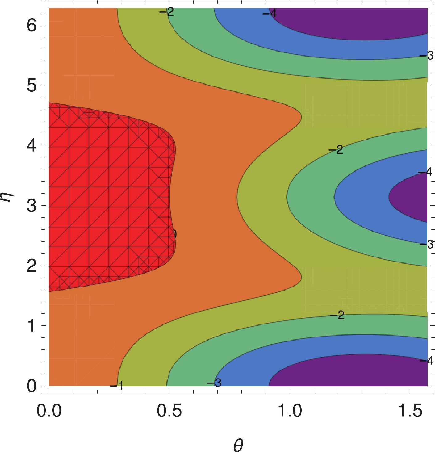
Figure 9. (color online) The space of (
$ \theta,\eta $ ). The red gridding range corresponds to$ R(\theta,\eta)>0 $ , while others correspond to$ R(\theta,\eta)<0. $ The critical points (
$ \pm 1, 0, 0 $ ) correspond to the universe dominated by the kinetic energy of$ \phi $ , and the perturbations of$ X,\;Y,\;\lambda $ around these points are governed by$ \quad\quad\quad\quad\frac{{\rm d}\delta X}{{\rm d}x} = 3X\delta X \,, $

(65) $ \quad\quad\quad\quad \frac{{\rm d}\delta Y}{{\rm d}x} = 3\delta Y \,, $

(66) $ \quad\quad\quad\quad \frac{{\rm d}\delta \lambda}{{\rm d}x} = \sqrt{6} X \Gamma_{A(1)} \delta \lambda \,. $

(67) Both of these points are unstable critical points. In the case of
$ \lambda_c\neq 0 $ , the critical point ($ 0, 0, \lambda_c $ ) is not of much interest, for it corresponds to the universe without$ \Omega_\phi $ , and it is a saddle point just like the ($ 0, 0, 0 $ ) point. The other two points have already been investigated in the literature. In summary, the multi-pole dark energy model does have stable attractor solutions just as the quintessence model in some parameter regions. We believe that the stability of the multi-pole model under the cosmological perturbations will also depend on the regions of the parameters and we will study it in further details in our next work. -
In the multi-pole dark energy model, a flat potential for the field
$ \sigma $ is no longer needed. After transforming to the canonical kinetic form, we could obtain a stable solution, which corresponded to the dark energy-dominated universe. A scaling solution could also be obtained. For example, if$ V(\sigma) = m^2\sigma^2/2 $ , and the required potential of$ \psi $ that leads to a constant equation of state$ w = w_c $ is$ V_s(\psi) $ , then function$ f $ should be chosen as$ \begin{array}{l} f(\sigma) = \sqrt{\dfrac{1}{2m^2V_s}} \dfrac{{\rm d}V_s}{{\rm d}\phi}\bigg(\phi = V_s^{-1}(m^2\sigma^2/2) \bigg)\,, \end{array} $

(68) where
$ V_s^{-1} $ is the inverse function of$ V_s $ .The whole dynamical system of Eqs. (27)-(29), Eq. (39), and Eqs. (41)-(42) seems to have infinite dimensions, since there is always a new variable
$ \Gamma_{A(n+1)} $ or$ \Gamma_{B(n+1)} $ that appears in the equation of$ {\rm d}\Gamma_{A(n)}/{\rm d}x $ or$ {\rm d}\Gamma_{B(n)}/{\rm d}x $ . If the function$ f $ or$ V $ has a maximum order of$ \sigma $ , e.g.$ \sigma^{N-1} $ , then$ \Gamma_{A(N)} = 0 $ or$ \Gamma_{B(N)} = 0 $ . As a result, the whole system is closed to form an autonomous system, and it has$ 2(N+1) $ -dimensions.In conclusion, we have proposed a multi-pole dark energy model. The cosmological evolution is obtained explicitly for the two pole model, while dynamical analysis on the whole system is performed for the multi-pole model. We find that this kind of dark energy model could have a stable solution, which corresponds to the universe dominated by the potential energy of the scalar field. Thus, the multi-pole dark energy model appears worthy of future investigation.
CJF would like to thank Prof. Eric V. Linder for very helpful comments.
Multi-pole dark energy
- Received Date: 2020-01-07
- Accepted Date: 2020-04-08
- Available Online: 2020-10-01
Abstract: A scalar field with a pole in its kinetic term is often used to study cosmological inflation; it can also play the role of dark energy, which is called the pole dark energy model. We propose a generalized model where the scalar field may have two or even multiple poles in the kinetic term, and we call it the multi-pole dark energy. We find that the poles can place some restrictions on the values of the original scalar field with a non-canonical kinetic term. After the transformation to the canonical form, we get a flat potential for the transformed scalar field even if the original field has a steep one. The late-time evolution of the universe is obtained explicitly for the two pole model, while dynamical analysis is performed for the multiple pole model. We find that it does have a stable attractor solution, which corresponds to the universe dominated by the potential of the scalar field.


 DownLoad: