


 Abstract
 HTML
HTML Reference
 Related
 PDF
PDF


-
The internal structure of baryon resonances has long been investigated by the excitation of resonances via the electromagnetic interaction. The electromagnetic transition form factors are the key source of information and yield essential information on the nature of strong interactions and quark confinement [1-3]. Furthermore, additional understandings of the substructure and underlying symmetry of nonstrange baryon resonances has been provided by means of the electromagnetic transition form factors [4]. Recent experiments in electro- and photo-production in the resonance region probe the spatial structure of baryons resonances by measuring the electromagnetic transition form factors [5-12]. Thus far, different quark models have been proposed and developed to investigate the electromagnetic transition between the nucleon and its resonances in theory, including the hypercentral constituent quark model [13], chiral effective field theory [14], light-front quark models [15-17], covariant spectator quark model [18], and soft-wall AdS/QCD model [19]. All of the mentioned quark models are perspective theoretical frameworks that efficiently describe the mass spectra of baryons and elastic form factors of the nucleon; however they predict a remarkably different Q2 dependence of the
$\gamma N \to {N^*},{{\Delta}^*}$ electrocouplings for nucleon and Δ resonances. In this study, our aim is to construct an appropriate quark model that not only predicts the excitation spectrum of nonstrange baryon, but also describes well the photoexcitation of the nucleon to a baryon resonance. The successful description of the mass spectra of light baryons motivated us to extend the model presented in Refs. [20, 21] to calculate the electroexcitation amplitudes for the nucleon and Δ resonances. Thus, in the present study we investigate the electromagnetic transition helicity amplitudes for the first radial and orbital excitations of the nucleon and Δ. The remainder of the paper is organized as follows. We first present the model constructed to solve the Schrödinger equation analytically for the eigenenergies and hyperradial component of the wave function, in Section 2. As the first task of the model, the spectrum of light baryons is described in Section 3. Subsequently, using the spin- and isospin-dependent wave functions, we calculated the longitudinal and transverse transition amplitudes for low-lying resonances of nucleon and Δ in Section 4. Section 5 is dedicated to discussing the results, and finally a conclusion is given in Section 6. -
In constituent quark models, the three-quark interaction potential contains a dominant confining SU(6)-invariant term, which accounts for the spacing between SU(6) multiplets and an small short-range spin dependent SU(6)-violating term, which generates the splittings within SU(6)-multiplets [22-27]. Without loss of generality, the antisymmetry of the total wave functions
${{\rm{\Psi }}_{{\rm{space}}}}{\rm{}}{{\rm{\Phi }}_{{S}{{U}_{{\rm{spin}} - {\rm{flavor}}}}\left( 6 \right)}}{{\rm{\Theta }}_{\rm color}}$ , with respect to the quark interchange, is given by the color factor Θcolor, and the product${{\rm{\Psi }}_{{\rm{space}}}}{{\rm{\Phi }}_{{S}{{U}_{{\rm{spin}} - {\rm{flavor}}}}\left( 6 \right)}}$ is symmetric. Furthermore, we can decompose the three quark states into the following SU(6) representations$6 \otimes 6 \otimes 6 = {20_{\rm{A}}} \oplus {70_{{\rm{MA}}}} \oplus {70_{{\rm{MS}}}} \oplus {56_{\rm{S}}}.$

(1) Considering the spin and flavor content of each SU(6)-representation, the three SU(6) representations can be decomposed into a SU(3) representation, as:
$ 20 = {}_{}^41 + {}_{}^48,\;\;\;56 = {}_{}^28 + {}_{}^410,\;\;\;70 = {}_{}^21 + {}_{}^28 + {}_{}^48 + {}_{}^210, $

(2) where the suffixes denote the multiplicity 2S +1 of the three-quark spin states. In the appendix, we provide the explicit form of the SU(6) configurations describing various baryon states. As supported by the lattice QCD calculations [28, 29], we consider the interaction potential of three quarks inside the baryon as:
$ {V_{3q}} = {V_{{SU}\left( 6 \right) - {\rm{invariant}}ا}} + {V_{{SU}\left( 6 \right) - {\rm{breaking}}}}, $

(3) where the SU(6)-invariant part of the interaction was composed of a linear confining term (dominant at large separations) and a one-gluon-exchange (OGE) term (dominant at short separations) given by a central Coulomb-like potential, whereas the SU(6)-breaking part is given by an spin- and isospin-dependent part, responsible for the hyperfine splitting of baryon masses:
$\begin{split}{V_{3q}} =& \mathop \sum \limits_{i < j} A{r_{ij}} - \frac{B}{{{r_{ij}}}} + \frac{{{{\rm e}^{ - \alpha {r_{ij}}}}}}{{{r_{ij}}}}\left[ C\left( {{{{\sigma}} _i}.{{{\sigma}} _j}} \right) + D\left( {{{{\tau}} _i}.{{{\tau}} _j}} \right)\right. \\&\left. + E\left( {{{{\sigma}} _i}.{{{\sigma}} _j}} \right)\left( {{{{\tau}} _i}.{{{\tau}} _j}} \right) \right]. \end{split} $

(4) Here, the δ-function represents spin and isospin exchange interactions [28] smeared by a Yukawa-type factor. Accordingly, the dynamics of the three-quark system is described as follows. After having removed the center of mass coordinate, the internal quark motion is described by the Jacobi coordinates ρ and λ, as:
$ {{\rho }} = \frac{1}{{\sqrt 2 }}({{{r}}_1} - {{{r}}_2}),\;{{\lambda }} = \frac{1}{{\sqrt 6 }}\left( {{{{r}}_1} + {{{r}}_2} - {\rm{}}2{{{r}}_3}} \right), $

(5) where ρ is the relative position of the pair in the two-body subsystem, and λ is the position of the third particle relative to the center of mass of the pair, where we supposed three constituents identical, mu = md. The hyperradius x and the hyperangle ξ are defined as [25-27]:
$ x = \sqrt {{\rho ^2} + {\lambda ^2}} ,\;\xi = \arctan \left( {\frac{\rho }{\lambda }} \right). $

(6) Using Jacobi coordinates, the Hamiltonian for three-interacting particles can be rewritten as:
${H_{3q}} = - \frac{1}{{2m}}\left[ {\frac{{{\partial ^2}}}{{\partial {x^2}}} + \frac{5}{x}\frac{\partial }{{\partial x}} - \frac{{{{{L}}^2}\left( {{{\rm{\Omega }}_\rho },{{\rm{\Omega }}_\lambda },\xi } \right)}}{{{x^2}}}} \right] + {V_{3q}}\left( {{{\rho }},{{\lambda }}} \right),$

(7) where
$m\left( { \equiv {m_u} = {m_d}} \right)$ is the common quark mass, and${V_{3q}}$ is the total interaction potential between the three quarks confined in a baryon. The term${{{L}}^2}\left( {{{\rm{\Omega }}_\rho },{{\rm{\Omega }}_\lambda },\xi } \right)$ is the generalized six-dimensional squared angular momentum operator, where its eigenfunctions are the well-known hyperspherical harmonics [27] that can be expressed as products of harmonic oscillators and Jacobi polynomials as:$\begin{split} {Y_{\left[ \gamma \right]{l_\rho }{l_\lambda }}}\left( {{{\rm{\Omega }}_\rho },{{\rm{\Omega }}_\lambda },\xi } \right) =& {\left[ {\frac{{2\left( {2\gamma + 2} \right){\rm{\Gamma }}\left( {\gamma + 2 - n} \right){\rm{\Gamma }}\left( {n + 1} \right)}}{{{\rm{\Gamma }}\left( {n + {l_\rho } + \frac{3}{2}} \right){\rm{\Gamma }}\left( {n + {l_\lambda } + \frac{3}{2}} \right)}}} \right]^{\frac{1}{2}}}\\&\times{Y_{{l_\rho }{m_\rho }}}\left( {{{\rm{\Omega }}_\rho }} \right){Y_{{l_\lambda }{m_\lambda }}}\left( {{{\rm{\Omega }}_\lambda }} \right)\\ & \times {\left( {{\rm{sin}}\xi } \right)^{{l_\rho }}}{\left( {{\rm{cos}}\xi } \right)^{{l_{\lambda }}}}P_n^{{l_\rho } + \frac{1}{2},{l_\lambda } + \frac{1}{2}}\left( {{\rm{cos}}2\xi } \right) \end{split}$

(8) with eigenvalues
$\gamma \left( {\gamma + 4} \right)$ . Here,$\gamma ( = 2n + {l_\rho } + {l_\lambda }$ , where n is a non-negative integer, and lρ and lλ are the angular momenta corresponding to the Jacobi coordinates ρ and λ) being the degree of the polynomial, is referred to as the grand orbital quantum number. In the hypercentral hypothesis, it is assumed that the confining potential is hypercentral and hence depends only on the hyperradius x. Therefore, we can factorize the spatial wave function into hyperradial and hyperangular parts as:${\varPsi _{3q}}\left( {{\bf{\rho }},{\bf{\lambda }}} \right) = {\psi _{\nu \gamma }}\left( x \right){\rm{}}{Y_{\left[ \gamma \right]{l_\rho }{l_\lambda }}}\left( {{{\rm{\Omega }}_\rho },{{\rm{\Omega }}_\lambda },\xi } \right).$

(9) Evidently, one can go beyond the hypercentral hypothesis by considering a non-hypercentral interaction, by means of a confining potential depending on the hyperangle ξ and/or Jacobi angles Ωρ and Ωλ, as well. A major feature of applying such an angle-dependent potential is to study the rotational-vibrational dynamics of a bound system. Thus, the addition of a non-hypercentral potential enables investigation of the contributions of parameters that arise from the angle-dependent potential into the observables of interest, such as the mass spectrum, electromagnetic form actors, helicity amplitudes, etc. However, in the hypercentral hypothesis, the angular-hyperangular part of the spatial wave function is determined by hyperspherical harmonics (8), and the hyperradial wave function is obtained via the solution of the hyperradial equation
$\left[ {\frac{{{\partial ^2}}}{{\partial {x^2}}} + \frac{5}{x}\frac{\partial }{{\partial x}} - \frac{{\gamma \left( {\gamma + 4} \right)}}{{{x^2}}} + 2m\left( {E - {V_{3q}}\left( x \right)} \right)} \right]{\psi _{\nu \gamma }}\left( x \right) = 0,$

(10) where ν and γ are the quantum numbers describing the hyperradial and orbital excitations, respectively. From Eq. (4), the hypercentral interaction contains an SU(6)-invariant "Columbic-linear" potential and an SU(6)-violating hyperfine interaction as:
$V\left( x \right) = \beta x - \frac{\tau }{x} + \frac{{{{\rm e}^{ - \alpha x}}}}{x}{A_{hyp}}\left( {S,T} \right),$

(11) with
${A_{hyp}}\left( {S,T} \right) \!=\! {A_S}\left( {{S^2} \!-\! \frac{9}{4}} \right) \!+\! {A_I}\left( {{T^2} - \frac{9}{4}} \right) \!+\! {A_{SI}}\left( {{S^2} \!-\! \frac{9}{4}} \right)\left( {{T^2} \!-\! \frac{9}{4}} \right).$

(12) The exact solution of the hyperradial Schrödinger equation (10) with nonlinear potential (11) can be obtained numerically [30]. However, to obtain closed form expressions for wavefunctions and energy eigenvalues, we must perform the calculations analytically. Hence, we used some approximations to omit the nonlinearity of the potential and deal with the problematic linear confining term and Yukawa-type smearing factor. To this end, we change the variable
$\delta = 1/x$ , and suppose a hypothetical length scale x0, around which a power series expansion must be presented for the 1/δ term. Setting$\varUpsilon = \delta - {\delta _0}$ , we found the power series expansion of 1/δ about$\varUpsilon=0$ up to the second order as:$x \cong \frac{3}{{{\delta _0}}} - \frac{3}{{{\delta _0}^2}}\delta + \frac{1}{{{\delta _0}^3}}{\delta ^2} + {\cal O}\left( {{\delta ^3}} \right),$

(13) where
${\delta _0} \equiv 1/{x_0}$ , and the model scale parameter x0 can be interpreted as a characteristic radius of the baryon, namely an effective length scale representing the distance within, (after) which the charge density of the baryon becomes substantial (as it loses a significant amount of its strength). It would also be useful to expand the exponential term in a Taylor series for small αx, as:${{\rm e}^{ - \alpha x}} \cong 1 - \alpha x + {\cal O}\left( {{{\left( {\alpha x} \right)}^2}} \right).$

(14) This condition is quite instructive when
$\alpha \ll 1\;{\rm{f}}{{\rm{m}}^{ - 1}}$ . Substituting the approximations (13) and (14), the hyperradial wave functions can be determined by the hypercentral Schrödinger equation:$\begin{split} &\left[ {\frac{{{\partial ^2}}}{{\partial {x^2}}} + \frac{5}{x}\frac{\partial }{{\partial x}} - \frac{{\gamma \left( {\gamma + 4} \right) + 2m\tilde \alpha }}{{{x^2}}} + 2m\left( {E - {V_0}_{ST} + \frac{{{{\tilde \tau }_{ST}}}}{x}} \right)} \right]\\&\quad\times{\psi _{\nu {\rm{\gamma }}}}\left( x \right) = 0\end{split}$

(15) with
$\begin{split} \tilde \alpha = &\alpha x_0^3,\;\;{V_0}_{ST} = 3\alpha {x_0} - \alpha {A_{hyp}}\left( {S,T} \right),\\{\tilde \tau _{ST}} =& \tau + 3\alpha x_0^2 - {A_{hyp}}\left( {S,T} \right).\end{split}$

(16) Eq. (15) is recognizable as the generalized six-dimensional Schrödinger equation with hyperCoulomb potential. Consequently, the eigenenergies and eigenfunctions can be obtained directly as [21]:
${E_{\nu ,\gamma ,S,T}} = 3\alpha {x_0} - \alpha {A_{hyp}}\left( {S,T} \right) - \frac{{m{{\left( {\tau + 3\alpha x_0^2 - {A_{hyp}}\left( {S,T} \right)} \right)}^2}}}{{2{{\left( {\nu + \tilde \gamma + 5/2} \right)}^2}}}$

(17) and
${\psi _{\nu \gamma ST}}\left( x \right) = {\left[ {\frac{{\nu !{{\left( {2h} \right)}^{2\tilde \gamma + 6}}}}{{\left( {2\nu + 2\tilde \gamma + 5} \right){\rm{\Gamma }}\left( {\nu + 2\tilde \gamma + 5} \right)}}} \right]^{\frac{1}{2}}}{x^{\tilde \gamma }}{{\rm e}^{ - hx}}L_\nu ^{2\tilde \gamma + 4}\left( {2hx} \right),$

(18) where
${A_{hyp}}\left( {S,T} \right)$ is given by Eq. (12), Γ(t) indicates the gamma function,$L_\nu ^{2\tilde \gamma + 4}\left( {2hx} \right)$ denotes associated Laguerre polynomials [31], and$\tilde \gamma + 2 = {\left[ {{{\left( {\gamma + 2} \right)}^2} + 2m\tilde \alpha } \right]^{\frac{1}{2}}},\;\;h = \frac{{m{{\tilde \tau }_{ST}}}}{{\nu + \tilde \gamma + 5/2}}.$

(19) As one notes, the hyperradial wavefunctions (18) depend not only on quantum numbers
$\left( {n,\gamma } \right)$ , but also on total spin S and isospin T. -
From Eq. (17), the spin- and isospin-dependent masses are given by
$M_{\nu ,\gamma ,S,T}^{} = 3m + E_{\nu ,\gamma ,S,T}^{}.$

(20) Considering the constituent quark mass at about 1/3 of the nucleon mass, the remaining free parameters are fitted to the spectrum, yielding the values listed in Table 1.
Parameter τ $\alpha/{\rm fm}^{ - 2} $ 

${x_0}/{\rm fm}$ 

$\mu/{\rm fm}^{ - 1}$ 

AS AI ASI Value 5.5 1.2 0.5 0.22 0.16 0.23 −0.15 Table 1. Fitted values of potential parameters obtained within analytical fixing procedure.
The results for light baryon masses are summarized in Table 2 and compared with experimental values [32]. Notwithstanding the applied approximations, the model provides a fair description for the observed resonances, especially for the lower part of the spectrum.
Baryon ${L_{2T\;2J}}$ 

ν γ S T $J^P$ 

MTheor. MExp. N(938) P11 0 0 $\dfrac{1}{2}$ 

$\dfrac{1}{2}$ 

${\dfrac{1}{2}^ + }$ 

939 939 N(1440) P11 1 0 $\dfrac{1}{2}$ 

$\dfrac{1}{2}$ 

${\dfrac{1}{2}^ + }$ 

1524 1410-1450 N(1520) D13 0 1 $\dfrac{1}{2}$ 

$\dfrac{1}{2}$ 

${\dfrac{3}{2}^ - }$ 

1511 1510-1520 N(1535) S11 0 1 $\dfrac{1}{2}$ 

$\dfrac{1}{2}$ 

${\dfrac{1}{2}^ - }$ 

1511 1525-1545 N(1650) S11 0 1 $\dfrac{3}{2}$ 

$\dfrac{1}{2}$ 

${\dfrac{1}{2}^ - }$ 

1651 1645-1670 N(1675) D15 0 1 $\dfrac{3}{2}$ 

$\dfrac{1}{2}$ 

${\dfrac{5}{2}^ - }$ 

1651 1670-1680 N(1680) F15 0 2 $\dfrac{1}{2}$ 

$\dfrac{1}{2}$ 

${\dfrac{5}{2}^ + }$ 

1763 1680-1690 N(1700) D13 0 1 $\dfrac{3}{2}$ 

$\dfrac{1}{2}$ 

${\dfrac{3}{2}^ - }$ 

1651 1650-1750 N(1710) P11 2 0 $\dfrac{3}{2}$ 

$\dfrac{1}{2}$ 

${\dfrac{1}{2}^ + }$ 

1772 1680-1740 N(1720) P13 0 2 $\dfrac{3}{2}$ 

$\dfrac{1}{2}$ 

${\dfrac{3}{2}^ + }$ 

1763 1700-1750 Δ(1232) P33 0 0 $\dfrac{3}{2}$ 

$\dfrac{3}{2}$ 

${\dfrac{3}{2}^ + }$ 

1249 1230-1234 Δ(1600) P33 1 0 $\dfrac{3}{2}$ 

$\dfrac{3}{2}$ 

${\dfrac{3}{2}^ + }$ 

1662 1500-1700 Δ(1620) S31 0 1 $\dfrac{1}{2}$ 

$\dfrac{3}{2}$ 

${\dfrac{1}{2}^ - }$ 

1673 1600-1660 Δ(1700) D33 0 1 $\dfrac{1}{2}$ 

$\dfrac{3}{2}$ 

${\dfrac{3}{2}^ - }$ 

1673 1670-1750 Δ(1900) S31 1 1 $\dfrac{1}{2}$ 

$\dfrac{3}{2}$ 

${\dfrac{1}{2}^ - }$ 

1842 1900-1902 Δ(1905) F35 0 2 $\dfrac{3}{2}$ 

$\dfrac{3}{2}$ 

${\dfrac{5}{2}^ + }$ 

1831 1855-1910 Δ(1910) P31 0 2 $\dfrac{3}{2}$ 

$\dfrac{3}{2}$ 

${\dfrac{1}{2}^ + }$ 

1831 1860-1910 Δ(1920) P33 2 0 $\dfrac{3}{2}$ 

$\dfrac{3}{2}$ 

${\dfrac{3}{2}^ + }$ 

1838 1900-1970 Δ(1950) F37 0 2 $\dfrac{3}{2}$ 

$\dfrac{3}{2}$ 

${\dfrac{7}{2}^ + }$ 

1831 1915-1950 Table 2. Mass spectrum of nonstrange baryons compared with experiment results [32].
-
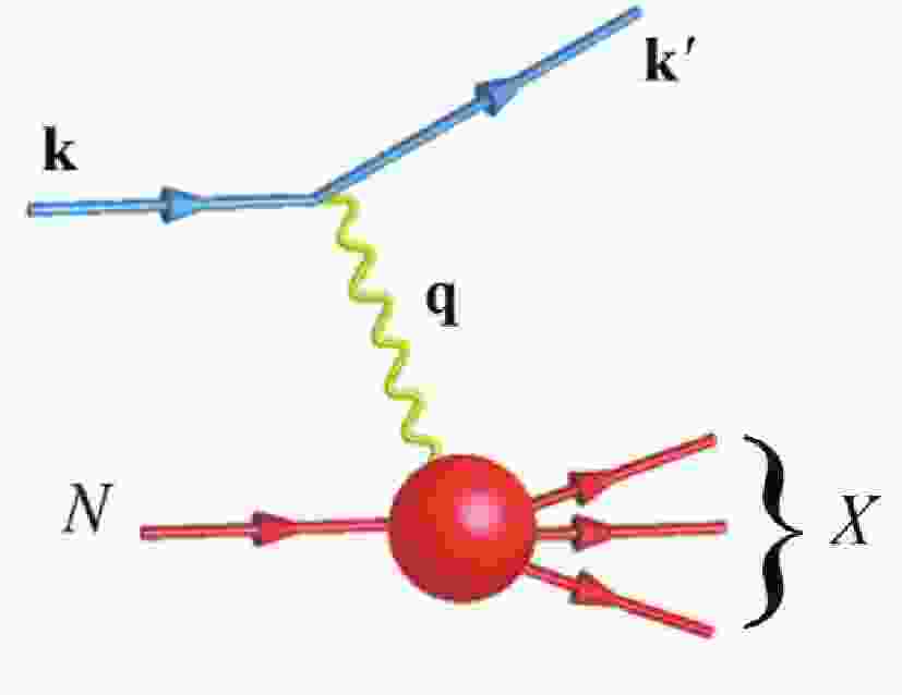
To determine the substructure of nucleon and Δ resonances, the electromagnetic transitions are investigated through the deep inelastic electron-nucleon scattering process, and the associated transition form factors are usually expressed in terms of Q2-dependent helicity amplitudes. The electromagnetic transition form factors provide quantitative information needed for explaining the substructure of resonant states. Fig. 1 shows a schematic representation of the one-photon-exchange for electron-nucleon inelastic scattering.
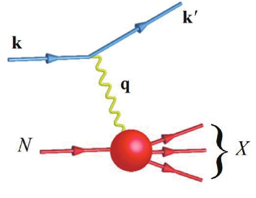
Figure 1. (color online) Schematic of deep inelastic electron-nucleon scattering process leading to electromagnetic transition of the ground state nucleon to nucleon and Δ resonances.
A virtual photon with momentum
${{q}} = {{k}}' - {{k}}$ and helicity${{\rm{\lambda }}_\gamma }\left( { = 0, \pm 1} \right)$ is absorbed by a ground state nucleon with helicity${{\rm{\lambda }}_N}\left( { = \pm \frac{1}{2}} \right)$ , leading to a resonant state with helicity${{\rm{\lambda }}_X}\left( { = \frac{1}{2},\frac{3}{2}} \right)$ where both the ground state nucleon and resonant state are considered in the rest frame, and the helicity is conserved via${{\rm{\lambda }}_X} = {{\rm{\lambda }}_\gamma } - {{\rm{\lambda }}_N}$ [33]. Transverse electrocouplings A1/2 and A3/2 are proportional to the helicity amplitudes that describe the transitions in the N* and Δ* rest frame between the initial transverse-photon and ground state nucleon (target) and the final resonant state of helicity 1/2 and 3/2, respectively. The longitudinal S1/2 electrocouplings are proportional to resonance electroexcitation amplitudes by means of longitudinal photons of zero helicity. Hence, the transverse and longitudinal helicity amplitudes are defined as:$\begin{split} {A_{3/2}} =& \left\langle {X,{J_z} = \frac{3}{2}{\rm{|}}{H_{em}}{\rm{|}}N,{J_z} = \frac{1}{2}} \right\rangle ,\\ {A_{1/2}} =& \left\langle {X,{J_z} = \frac{1}{2}{\rm{|}}{H_{em}}{\rm{|}}N,{J_z} = - \frac{1}{2}} \right\rangle ,\\ {S_{1/2}} =& \left\langle {X,{J_z} = \frac{1}{2}{\rm{|}}{H_{em}}{\rm{|}}N,{J_z} = \frac{1}{2}} \right\rangle, \end{split}$

(21) where X indicates the nucleon and Δ resonances, and Hem denotes the electromagnetic interaction given by a direct photon-quark coupling and is written in the non-relativistic approximation as [34, 35]:
${H_{em}} = - \mathop \sum \limits_{j = 1}^3 \left\{ {\frac{{{e_j}}}{{2{m_j}}}\left( {{{{p}}_j}.{{{A}}_j} + {{{A}}_j}.{{{p}}_j}} \right) + {\mu _j}{{{s}}_j}.\left( {\nabla \times {{{A}}_j}} \right)} \right\},$

(22) where ej, mj, sj, pj and μj=gej/2mj denote the electric charge, mass, spin, momentum, and the magnetic moment of the j-th constituent, respectively, and
${{{A}}_j} \equiv {{A}}\left( {{{{r}}_j}} \right)$ is the vector potential of the electromagnetic field of a photon. Considering the monochromatic photon field, after replacing${{p}}/m$ with$i{k_0}{{r}}$ , the transverse (longitudinal) coupling is obtained by inserting the radiation field for the absorption of a right-handed (longitudinally polarized) photon into Eq. (22) [34]. For three identical constituents, the symmetry of the wave functions allows us to write${\cal H} = 3{{\cal H}_3}$ (${\cal H} \equiv {H_{em}}$ defined in Eq. (22)), and thus the electromagnetic transition operator reads:${\cal H}_{}^n = 6\sqrt {\frac{\pi }{{{k_0}}}} \mu {e_3}\left[ {nk{s_{3, + }}\hat U + \frac{1}{g}{{\left( { - 1} \right)}^n}{{\hat T}_n}} \right],$

(23) here
$n = + 1\left( 0 \right)$ indicates the transverse (longitudinal)${\cal H}_{}^t$ (${\cal H}_{}^l$ ) coupling and${\hat T_0} \equiv {\hat T_z}$ . In Eq. (23),${s_{3, + }} = {s_{3,x}} + i{s_{3,y}}$ and e3 correspond to spin operator and the charge of third quark, respectively, and$\hat U$ and$\hat T$ are operators acting on the spatial part of wavefunction given by:$\hat U = {{\rm e}^{ - {\rm i}k\eta {\lambda _z}}},\;{\hat T_n} = im{k_0}\eta {\lambda _n}{{\rm e}^{ - {\rm i}k\eta {\lambda _z}}},\;n = 0, \pm 1,$

(24) with
$\eta = \sqrt {2/3} $ . Because the electromagnetic transition operator${\cal H}_{}^n$ in Eq. (23), acts both on the spin-flavor, Eq. (A3), and the space part of the nucleon wave functions, Eq. (9), one has to separate these two parts by decoupling the wave function. After doing so, the transverse helicity amplitudes can be expressed in terms of radial integrals${A_m} = \left\langle {f{\rm{|}}{\cal H}_{}^{ + 1}{\rm{|}}i} \right\rangle = {\alpha _m}{\cal A} + {\beta _m}{\cal B},$

(25) $ {\cal A} = 6\sqrt {\frac{\pi }{{{k_0}}}} \mu \frac{1}{g}\left\langle {f{\rm{|}}{{\hat T}_{ + 1}}{\rm{|}}i} \right\rangle ,\;\;\;\;\;{\cal B} = 6\sqrt {\frac{\pi }{{{k_0}}}} \mu k\left\langle {f{\rm{|}}\hat U{\rm{|}}i} \right\rangle, $

(26) where index m denotes the helicity (1/2,3/2), i and f represent initial and final states, and
${\cal A}$ and${\cal B}$ represent the orbit- and spin-flip spatial amplitudes, respectively. The longitudinal helicity amplitude can be expressed in terms of single spatial amplitude as:${A_l} = \left\langle {f{\rm{|}}{H^0}{\rm{|}}i} \right\rangle = 6{\gamma _l}\sqrt {\frac{\pi }{{{k_0}}}} \mu \frac{1}{g}\left\langle {f{\rm{|}}{{\hat T}_0}{\rm{|}}i} \right\rangle. $

(27) The coefficients αm, βm, and γl given in Table 3 contain the contributions of the spin-flavor matrix elements and of Clebsh-Gordon coefficients. Using the hyperradial wave functions given by Eq. (18) and hyperspherical harmonics (8), we can evaluate the matrix elements of the operators
$\hat U$ and${\hat T_n}$ of Eq. (24), where the initial state is the ground state. The angular-hyperangular integrals can be evaluated in terms of the integral representation of the ordinary Bessel functions, whose derivatives with respect to z result inResonance State A1/2 A3/2 Al α1/2 β1/2 α3/2 β3/2 γl N (1440) P11 ${}_{}^2{8_{1/2}}\left[ {56,{0^ + }} \right]$ 

0 $\dfrac{1}{3}$ 

0 0 $\dfrac{1}{3}$ 

N (1520) D13 ${}_{}^2{8_{1/2}}\left[ {70,{1^ - }} \right]$ 

$\dfrac{{ - 1}}{{3\sqrt 6 }}$ 

$\dfrac{1}{{3\sqrt 3 }}$ 

$\dfrac{{ - 1}}{{3\sqrt 2 }}$ 

0 $\dfrac{{ - 1}}{{3\sqrt 3 }}$ 

N (1535) S11 ${}_{}^2{8_{1/2}}\left[ {70,{1^ - }} \right]$ 

$\dfrac{{ - 1}}{{3\sqrt 3 }}$ 

$\dfrac{{ - 1}}{{3\sqrt 6 }}$ 

0 0 $\dfrac{{ - 1}}{{3\sqrt 6 }}$ 

${\Delta}\left( {1232} \right)\;{{\rm{P}}_{33}}$ 

${}_{}^4{10_{3/2}}\left[ {56,{0^ + }} \right]$ 

0 $\dfrac{{ - \sqrt 2 }}{9}$ 

0 $\dfrac{{ - \sqrt 2 }}{{3\sqrt 3 }}$ 

0 ${\Delta}\left( {1600} \right)\;{{\rm{P}}_{33}}$ 

${}_{}^4{10_{3/2}}\left[ {56,{0^ + }} \right]$ 

0 $\dfrac{{ - \sqrt 2 }}{9}$ 

0 $\dfrac{{ - \sqrt 2 }}{{3\sqrt 3 }}$ 

0 ${\Delta}\left( {1620} \right)\;{{\rm{S}}_{31}}$ 

${}_{}^2{10_{1/2}}\left[ {70,{1^ - }} \right]$ 

$\dfrac{1}{{3\sqrt 3 }}$ 

$\dfrac{{ - 1}}{{9\sqrt 6 }}$ 

0 0 $\dfrac{1}{{3\sqrt 6 }}$ 

${\Delta}\left( {1700} \right)\;{{\rm{D}}_{33}}$ 

${}_{}^2{10_{3/2}}\left[ {70,{1^ - }} \right]$ 

$\dfrac{1}{{3\sqrt 6 }}$ 

$\dfrac{1}{{9\sqrt 3 }}$ 

$\dfrac{1}{{3\sqrt 2 }}$ 

0 $\dfrac{{ - 1}}{{3\sqrt 3 }}$ 

Table 3. Spin-flavor coefficients of transverse and longitudinal helicity amplitudes for nucleon resonances; proton-target couplings. Columns 1 and 2 denote the state of resonances in the notation of PDG and are labeled as
${}_{}^{2S + 1}{\rm{dim}}{\left\{ {S{U_F}\left( 3 \right)} \right\}_J}\left[ {{\rm{dim}}\left\{ {S{U_{SF}}\left( 6 \right)} \right\},{L^P}} \right]$ .$\displaystyle\mathop \int \nolimits_0^\pi {\rm d}\xi {\rm{si}}{{\rm{n}}^{2\beta }}\xi {\rm{co}}{{\rm{s}}^\alpha }\xi {{\rm e}^{{\rm i}z{\rm cos}\xi }} = \sqrt \pi \varGamma \left( {\beta + \frac{1}{2}} \right){2^\beta }\frac{{{{\rm d}^\alpha }}}{{{\rm d}{z^\alpha }}}\left[ {\frac{{{J_\beta }\left( z \right)}}{{{z^\beta }}}} \right]{\left( { - i} \right)^\alpha }.$

(28) Using the recurrence relations of spherical Bessel functions, we obtain
$ \displaystyle\mathop \int \nolimits_0^{\pi /2} {\rm d}\xi \;{\rm{si}}{{\rm{n}}^2}\xi {\rm{co}}{{\rm{s}}^2}\xi {j_0}\left( {z{\rm{cos}}\xi } \right) = \frac{\pi }{2}\frac{{{J_2}\left( z \right)}}{{{z^2}}}. $

(29) Finally, integrating over the hyperradius, all transverse and longitudinal helicity amplitudes, Eqs. (25) and (27), can be obtained analytically and expressed in terms of the hypergeometric functions as:
$\begin{split} &\displaystyle\mathop \int \nolimits_0^\infty {x^{\tilde \gamma + 3}}{{\rm e}^{ - sx}}{J_2}\left( {\eta kx} \right){\rm d}x\\ =& - \frac{{\varGamma \left( {\tilde \gamma + 6} \right)}}{{2\left( {\tilde \gamma + 2} \right)\left( {\tilde \gamma + 3} \right)}}{s^{ - \left( {\tilde \gamma + 6} \right)}}\left[ {{{\left( {\left( {2\tilde \gamma + 7} \right){\eta ^2}{k^2} - 2{s^2}} \right)}}} \right.\\ &\times {}_2{F_1}\left( {\frac{{\tilde \gamma + 6}}{2},\frac{{\tilde \gamma + 7}}{2};2; - \frac{{{\eta ^2}{k^2}}}{{{s^2}}}} \right)\\ &+ 2{\left( {{\eta ^2}{k^2} + {s^2}} \right)}\left. {{}_2{F_1}\left( {\frac{{\tilde \gamma + 6}}{2},\frac{{\tilde \gamma + 7}}{2};1; - \frac{{{\eta ^2}{k^2}}}{{{s^2}}}} \right)} \right]. \end{split}$

(30) -
We calculated the longitudinal S1/2 and transverse A1/2, 3/2 helicity amplitudes for the electromagnetic excitations of nonstrange baryon resonances up to the second resonance region. We consider the target proton and the resonant state at rest and neglect the relativistic effects associated with the motion of the constituent quarks. With these constraints, the interpretation of the helicity amplitudes is valid in the Breit (or brick-wall) frame. Hence, the amplitudes are evaluated in the Breit frame:
${k^2} = {Q^2} + \frac{{{{\left( {{W^2} - {M^2}} \right)}^2}}}{{2\left( {{W^2} + {M^2}} \right) + {Q^2}}},$

(31) where M is the nucleon mass, W is the resonance mass, k0 and k are the energy and momentum of the virtual photon, respectively, and
${Q^2} = {k^2} - {k_0}^2$ . For consistency, in the calculations we use the values given by the model and not the phenomenological masses. The matrix elements of the electromagnetic transition operator between any two three-quark states are expressed in terms of some expressions involving the hypergeometric functions. Accordingly, the Q2 dependence of the three helicity amplitudes, in the range Q2 < 5.0 GeV2, are presented for resonant states and compared with experimental data points extracted from the electroproduction of mesons off protons. Furthermore, one can compare the$\gamma p \to {N^*},{\varDelta ^*}$ transverse helicity amplitudes A1/2 and A3/2 at the real photon point (Q2 = 0) with the proton photocouplings given by the Particle Data Group [32]. -
In Fig. 2 graphically portrays the Q2 evolution of the helicity amplitudes for the Roper N1440P11 resonance. As customary in constituent quark models, the model fails to describe the data for proton-Roper transition form factors in the low Q2 region and the internal structure of the resonance remains puzzling. However, for both helicity amplitudes, we achieved a qualitatively similar behavior to that obtained by experiments [2, 5, 36], in the high Q2 region. For the Roper resonance, deviations from the experimental data may be attributed to the inaccuracies arising from the fact that the state may does not belong to the pure SU(6)-multiplet
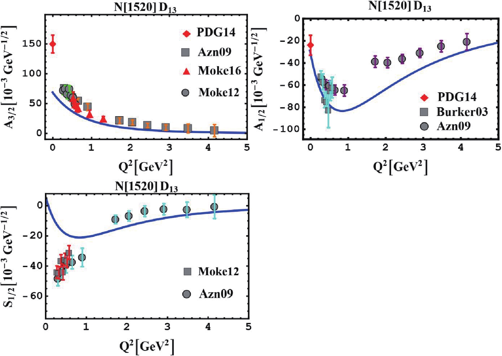
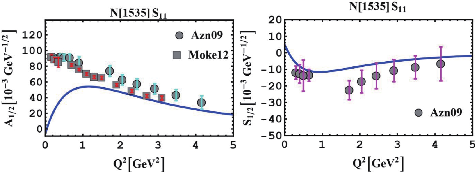
$\left[ {56,{0^ + }} \right]$ and may contain contributions from other SU(6)-multiplets. Moreover, it is likely that contributions beside the single quark transitions may contribute to the amplitudes. However, a fairly good phenomenological description of the helicity amplitudes of the Roper resonance may be found when the state is considered as a constituent quark-gluon core surrounded by the meson cloud [37], and/or meson-baryon molecule-like state [38]. The results for the first orbitally excited states, namely two negative parity states, N(1520)D13 and N(1535)S11 resonances, are given in Figs. 3 and 4, respectively. The theoretical amplitudes agree well with experimental data [2, 5, 6, 32, 39, 40], whereas problems are encountered for the strength of the S1/2 of the N(1520)D13 and A1/2 of the N(1535)S11 at low momentum transfer. However, one can find more consistent results for N(1520)D13 helicity amplitudes and form factors in Ref. [41], where a covariant spectator quark model is applied to the${\gamma ^*}N \to N\left( {1520} \right)$ reaction in the spacelike region. Furthermore, a more consistent description of the${\gamma ^*}N \to N\left( {1535} \right)$ transition has been achieved within the soft-wall AdS/QCD model [42].
-
Figure 5 shows the transverse amplitudes A3/2 and A1/2 for Δ(1232)P33 states. At the photon point, the calculated values agree with the PDG data [32]. The low Q2 behavior is fairly well reproduced [43-45], while the medium-high Q2 behavior decreases too slowly with respect to the data [36]. Thus, the helicity amplitudes are generally underestimated by the model. In this study, the theoretical value of the longitudinal transition amplitude S1/2 is zero, while it has been proven in the Refs. [46-48] that the longitudinal helicity amplitude is entirely determined by the pionic meson cloud. It is worthwhile pointing out that the ratio

${R_{\rm EM}} = - \frac{{{G_E}}}{{{G_M}}} = \frac{{{{{A}}_{1/2}} - {A}_{3/2}/\sqrt 3 }}{{{A_{1/2}} + \sqrt 3 {A}_{3/2}}},$

(31) at the photon point, accounts for the possible deformation. Here, we found the theoretical value of the ratio to be approximately REM = 0.01, which is not far from the experimental value REM = 0.025 ± 0.005 [32].
The Δ(1600)P33 resonance is considered the Roper-like excitation of Δ(1232). To date, there is no experimental data available on photon virtualities Q2 > 0 for the
${\gamma ^*}N \to {\Delta}\left( {1600} \right){\rm{}}$ reaction, and one can notice that the Δ(1600)P33 helicity amplitudes in Fig. 6, are in fair agreement with the PDG data points [32]. From Figs. 7 and Fig. 8 showing Δ(1620) S31 and Δ(1700) D33 helicity amplitudes indicate that there is agreement with the PDG data points and scarce experimental data extracted from the JLab-CLAS detector [32, 49-52], if we neglect the low photon virtualities Q2 < 1 for the Δ(1620) S31 longitudinal amplitude. Like other calculations within a constituent quark model, in the present calculation, the discrepancies in the low momentum region are considered to be pointing out the lack of pion-coupling effects. Obviously, a meson-cloud surrounding the three constituent quarks and mediating long-distance interactions is expected to have important contributions in the low-momentum region [46, 48]. In summary, taking the meson-cloud contributions into account as well as the inclusion of spin- and isospin-dependent terms in the hypercentral potential allows a significantly improved description of helicity amplitudes for photo- and electroproduction of nucleon and Δ resonances excited from protons. However, one should keep in mind that the present model is an analytical model containing some effective free parameters, and the parameter fitting procedure affects the model predictions for the observables. Accordingly, the free parameters could be refitted anytime through different fixing procedures to achieve a better reproduction of the data. Nevertheless, there is a fairly good agreement in the magnitude and sign of the photocouplings between the calculated helicity amplitude and the PDG data points. Moreover, the calculated Q2 evolution of the transition form factors provide a good account of the experimental data points. The results are also comparable with those obtained by other successful theoretical approaches.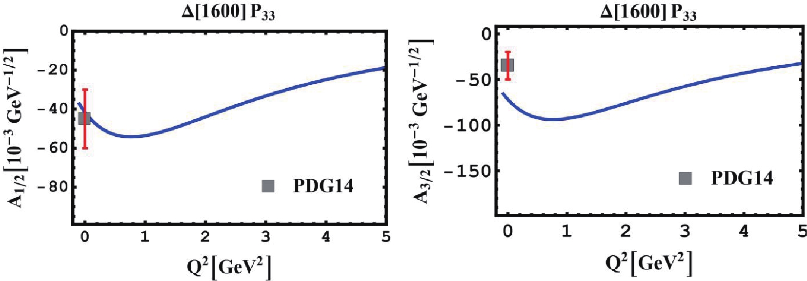
Figure 6. (color online) Proton helicity ampitudes A1/2 and A3/2 for Δ(1600) P33 resonance. PDG points [32] are also shown.

-
We investigated the Q2 behavior of the electromagnetic transition form factors of nucleon and Δ resonances. Theoretical results were compared with available experimental data on the meson electroproduction off protons, and it was shown that applying the spin- and isospin-dependent wavefunctions leads to a better reproduction of transverse and longitudinal helicity amplitudes for nucleon and Δ resonances, and excellent agreement with the existing data was achieved.
-
Baryons are considered as the bound states of three quarks, and each baryon state is a superposition of
$SU $ (6)-configurations, factorized as:$\tag{A1}{{\rm{\Psi }}_{3q}} = {\Psi _{3q}}\left( {{\bf{\rho }},{\bf{\lambda }}} \right){\rm{}}.{\chi _{\rm spin}}.{\rm{}}{\phi _{\rm isospin}}{\rm{}}.{\rm{}}{{\rm{\Theta }}_{\rm color}}.$

(A1) Various parts of the three-quark wave function must be combined to obtain an entirely antisymmetric wavefunction. To this aim, we need to study the behavior of the different factors with respect to the permutations of three objects (that is, with respect to the group S3) [13]. Generally, there is three symmetry types for any three-particle wavefunction: symmetry (S), antisymmetry (A), mixed symmetry with symmetric pair (MS), and mixed symmetry with antisymmetric pair (MA). Choosing the antisymmetric color singlet combination for the color part Θcolor, the antisymmetric combination is disregarded, and there would be only two states available for three particles. The remaining three-quark spin and isospin states, with definite S3-symmetry, are defined as:
$\tag{A2}\begin{split}{\vartheta _{\rm S}} =& \left| {\left( {\left( {\frac{1}{2},\frac{1}{2}} \right)1,\frac{1}{2}} \right)\frac{3}{2}} \right\rangle ,\;\;\;\;\;\;{\vartheta _{\rm MS}} = \left| {\left( {\left( {\frac{1}{2},\frac{1}{2}} \right)1,\frac{1}{2}} \right)\frac{1}{2}} \right\rangle {\rm{}},\\{\vartheta _{\rm MA}} =& \left| {\left( {\left( {\frac{1}{2},\frac{1}{2}} \right)0,\frac{1}{2}} \right)\frac{1}{2}} \right\rangle .\end{split}$

(A2) In the case of the spin- and isospin (flavour)-independent interactio, we have to introduce products of spin and isospin states with definite S3-symmetry. In the following, the explicit forms are presented only for the case that both spin and isospin factors have mixed symmetry, where the remaining ones are trivial:
$\tag{A3} \begin{split} {{\rm{\Omega }}_{\rm S}} = \frac{1}{{\sqrt 2 }}\left[ {{\chi _{\rm MA}}\;{\phi _{\rm MA}} + {\chi _{\rm MS}}\;{\phi _{\rm MS}}} \right]{\rm{}},\;\;{{\rm{\Omega }}_A} = \frac{1}{{\sqrt 2 }}\left[ {{\chi _{\rm MA}}\;{\phi _{\rm MS}} - {\chi _{\rm MS}}\;{\phi _{\rm MA}}} \right],\\ {{\rm{\Omega }}_{\rm MS}} = \frac{1}{{\sqrt 2 }}\left[ {{\chi _{\rm MA}}\;{\phi _{\rm MA}} - {\chi _{\rm MS}}\;{\phi _{\rm MS}}} \right],\;\;{{\rm{\Omega }}_{\rm MA}} = \frac{1}{{\sqrt 2 }}\left[ {{\chi _{\rm MA}}\;{\phi _{\rm MS}} + {\chi _{\rm MS}}\;{\phi _{\rm MA}}} \right]. \end{split} $

(A3) The explicit form of three-quark states with positive and negative parity is given in Table 4.
Resonance $L_{{S_3}}^P$ 

S T SU(6) configurations P11 $0_S^ + $ 

$\dfrac{1}{2}$ 

$\dfrac{1}{2}$ 

${\psi _{00}}\;{Y_{\left[ 0 \right]00}}\;{{\rm{\Omega }}_S}$ 

$0_S^ +$ 

$\dfrac{1}{2}$ 

$\dfrac{1}{2}$ 

${\psi _{10}}\;{Y_{\left[ 0 \right]00}}\;{{\rm{\Omega }}_S}$ 

$0_S^ +$ 

$\dfrac{1}{2}$ 

$\dfrac{1}{2}$ 

${\psi _{20}}\;{Y_{\left[ 0 \right]00}}\;{{\rm{\Omega }}_S}$ 

$0_M^ + $ 

$\dfrac{1}{2}$ 

$\dfrac{1}{2}$ 

${\psi _{02}}\;\dfrac{1}{{\sqrt 2 }}\left[ {{Y_{\left[ 2 \right]00}}\;{{\rm{\Omega }}_{MS}} + {Y_{\left[ 2 \right]11}}\;{{\rm{\Omega }}_{MA}}} \right]$ 

$2_M^ + $ 

$\dfrac{3}{2}$ 

$\dfrac{1}{2}$ 

${\psi _{02}}\dfrac{1}{{\sqrt 2 }}\left[ {\dfrac{1}{{\sqrt 2 }}\left( {{Y_{\left[ 2 \right]20}} - {Y_{\left[ 2 \right]02}}} \right){\phi _{MS}} + {Y_{\left[ 2 \right]11}}{\phi _{MA}}} \right]{\chi _S}$ 

P33 $0_S^ + $ 

$\dfrac{3}{2}$ 

$\dfrac{3}{2}$ 

${\psi _{00}}\;{Y_{\left[ 0 \right]00}}{\chi _S}\;{\phi _S}$ 

$0_S^ + $ 

$\dfrac{3}{2}$ 

$\dfrac{3}{2}$ 

${\psi _{10}}\;{Y_{\left[ 0 \right]00}}\;{\chi _S}\;{\phi _S}$ 

$0_S^ + $ 

$\dfrac{3}{2}$ 

$\dfrac{3}{2}$ 

${\psi _{20}}\;{Y_{\left[ 0 \right]00}}\;{\chi _S}\;{\phi _S}$ 

$2_S^ + $ 

$\dfrac{3}{2}$ 

$\dfrac{3}{2}$ 

${\psi _{02}}\;\dfrac{1}{{\sqrt 2 }}\left[ {{Y_{\left[ 2 \right]20}} + {Y_{\left[ 2 \right]02}}} \right]{\chi _S}\;{\phi _S}$ 

$2_M^ + $ 

$\dfrac{1}{2}$ 

$\dfrac{3}{2}$ 

${\psi _{02}}\;\dfrac{1}{{\sqrt 2 }}\left[ {\dfrac{1}{{\sqrt 2 }}\left( {{Y_{\left[ 2 \right]20}} - {Y_{\left[ 2 \right]02}}} \right){\chi _{MS}} + {Y_{\left[ 2 \right]11}}\;{\chi _{MA}}} \right]{\phi _S}$ 

S11 $1_M^ - $ 

$\dfrac{1}{2}$ 

$\dfrac{1}{2}$ 

${\psi _{01}}\dfrac{1}{{\sqrt 2 }}\left[ {{Y_{\left[ 1 \right]10}}{{\rm{\Omega }}_{MA}} + {Y_{\left[ 1 \right]01}}{{\rm{\Omega }}_{MS}}} \right]$ 

$1_M^ - $ 

$\dfrac{1}{2}$ 

$\dfrac{1}{2}$ 

${\psi _{11}}\dfrac{1}{{\sqrt 2 }}\left[ {{Y_{\left[ 1 \right]10}}{{\rm{\Omega }}_{MA}} + {Y_{\left[ 1 \right]01}}{{\rm{\Omega }}_{MS}}} \right]$ 

$1_M^ - $ 

$\dfrac{3}{2}$ 

$\dfrac{1}{2}$ 

${\psi _{01}}\dfrac{1}{{\sqrt 2 }}\left[ {{Y_{\left[ 1 \right]10}}{\phi _{MA}} + {Y_{\left[ 1 \right]01}}{\phi _{MS}}} \right]{\chi _S}$ 

$1_M^ - $ 

$\dfrac{3}{2}$ 

$\dfrac{1}{2}$ 

${\psi _{11}}\dfrac{1}{{\sqrt 2 }}\left[ {{Y_{\left[ 1 \right]10}}{\phi _{MA}} + {Y_{\left[ 1 \right]01}}{\phi _{MS}}} \right]{\chi _S}$ 

S31 $1_M^ - $ 

$\dfrac{1}{2}$ 

$\dfrac{3}{2}$ 

${\psi _{01}}\dfrac{1}{{\sqrt 2 }}\left[ {{Y_{\left[ 1 \right]10}}{\chi _{MA}} + {Y_{\left[ 1 \right]01}}{\chi _{MS}}} \right]{\phi _S}$ 

$1_M^ - $ 

$\dfrac{1}{2}$ 

$\dfrac{3}{2}$ 

${\psi _{11}}\dfrac{1}{{\sqrt 2 }}\left[ {{Y_{\left[ 1 \right]10}}{\chi _{MA}} + {Y_{\left[ 1 \right]01}}{\chi _{MS}}} \right]{\phi _S}$ 

D13 $1_M^ - $ 

$\dfrac{1}{2}$ 

$\dfrac{1}{2}$ 

${\psi _{01}}\dfrac{1}{{\sqrt 2 }}\left[ {{Y_{\left[ 1 \right]10}}{{\rm{\Omega }}_{MA}} + {Y_{\left[ 1 \right]01}}{{\rm{\Omega }}_{MS}}} \right]$ 

$1_M^ - $ 

$\dfrac{1}{2}$ 

$\dfrac{1}{2}$ 

${\psi _{11}}\dfrac{1}{{\sqrt 2 }}\left[ {{Y_{\left[ 1 \right]10}}{{\rm{\Omega }}_{MA}} + {Y_{\left[ 1 \right]01}}{{\rm{\Omega }}_{MS}}} \right]$ 

$1_M^ - $ 

$\dfrac{3}{2}$ 

$\dfrac{1}{2}$ 

${\psi _{01}}\dfrac{1}{{\sqrt 2 }}\left[ {{Y_{\left[ 1 \right]10}}{\phi _{MA}} + {Y_{\left[ 1 \right]01}}{\phi _{MS}}} \right]{\chi _S}$ 

$1_M^ - $ 

$\dfrac{3}{2}$ 

$\dfrac{1}{2}$ 

${\psi _{11}}\dfrac{1}{{\sqrt 2 }}\left[ {{Y_{\left[ 1 \right]10}}{\phi _{MA}} + {Y_{\left[ 1 \right]01}}{\phi _{MS}}} \right]{\chi _S}$ 

D33 $1_M^ - $ 

$\dfrac{1}{2}$ 

$\dfrac{3}{2}$ 

${\psi _{01}}\dfrac{1}{{\sqrt 2 }}\left[ {{Y_{\left[ 1 \right]10}}{\chi _{MA}} + {Y_{\left[ 1 \right]01}}{\chi _{MS}}} \right]{\phi _S}$ 

$1_M^ - $ 

$\dfrac{1}{2}$ 

$\dfrac{3}{2}$ 

${\psi _{11}}\dfrac{1}{{\sqrt 2 }}\left[ {{Y_{\left[ 1 \right]10}}{\chi _{MA}} + {Y_{\left[ 1 \right]01}}{\chi _{MS}}} \right]{\phi _S}$ 

Table 4. Three-quark states with positive and negative parity. Column 2 lists the angular momentum, parity, and S3-symmetry;
$L_{{S_3}}^P$ , and Columns 3 and 4 represent the spin, S, and isospin, T. States are shown in the last column and are written in terms of the hyperradial wave functions ψνγ, of the combinations (${Y_{\left[ \gamma \right]{l_\rho }{l_\lambda }}}$ ) S3 of the hyperspherical harmonics${Y_{\left[ \gamma \right]{l_\rho }{l_\lambda }}}$ with definite S3-symmetry, and of the spin and isospin states.
Analytical investigation of γN→N*,Δ* transition helicity amplitudes
- Received Date: 2020-02-26
- Available Online: 2020-07-01
Abstract: We study the structure of nonstrange baryons by analytically calculating the electromagnetic transition helicity amplitudes of the nucleon and Δ resonances. We employ an improved hypercentral constituent quark model and obtain the corresponding eigenenergies and eigenfunctions in closed forms. Then, we calculate the transverse and longitudinal helicity amplitudes for nucleon and Δ resonances. The comparison of evaluated observables and experimental data indicates good agreement between the proposed model and available data.


 DownLoad: