


 Abstract
 HTML
HTML Reference
 Related
 PDF
PDF


-
A complete gravitational collapse of a massive or a supermassive star leads to one of the following fates: a neutron star, black hole or naked singularity, depending on the initial mass of the star and on the various initial conditions of its physical parameters [1]. From the mathematical and astrophysical perspectives, the task of distinguishing the scenarios of formation of a black hole and naked singularities remains enigmatic. In this context we should emphasize that the recent measurement of the black hole shadow has ruled out the possibility that M87 is a naked singularity. Also, all LIGO measurements predict a black-hole-like nature of the compact objects. However, from the theoretical point of view, the question remains whether a given configuration of matter that collapses leads to the formation of a horizon or not. In other words, whether the horizons are formed prior to the curvature singularity or later. Researchers also pondered whether a black hole can convert into a naked singularity. Numerous thought experiments involving the absorption of spinning or charged particles in an extremal black hole lead to the destruction of the horizon [2-6]. However, considerations of back-reaction or self-conservative force avoid such a conclusion [7].
Although there are numerous astrophysical candidates for black holes, there are none for a naked singularity. This still does not discard the possibility of existence of visible singularities, since these are valid predictions of the Einstein theory of General Relativity. In order to distinguish an astrophysical black hole from a naked singularity, few important schemes are proposed: the phenomenon of gravitational lensing and formation of shadow images [8-12]; detection of hard X- and gamma-rays from the inner regions of accretion disks surrounding compact objects [13]; investigation of gravitational waves emitted from compact objects [14]; and the spin precession frequency of a stationary test gyroscope which is frame dragged in the ergo-region of the spinning black hole [15-20]. However, from the theoretical perspective, only a theory of quantum gravity can ultimately explain the process of complete gravitational collapse. Observationally, the Gravity Probe B detected and measured the geodetic precession frequency of a gyroscope relative to Earth [21]. However, these results are not directly applicable to black holes. Also, the measurement of Gravity Probe B is a weak field result, while we are interested in the region near the ergo-sphere, where strong field effects are present. The relativistic gyro-frequency diverges in the ergo-region of the black hole, while for a naked singularity, it diverges near the singularity itself. In recent years, the gyro-frequency has been calculated for various spinning black holes and naked singularities with interesting observable consequences.
The pioneering idea of Kaluza and Klein (KK) was an attempt to unify the two fundamental forces, electromagnetism and gravity, by introducing one extra spatial dimension to the four-dimensional spacetime structure. The hypothesis of KK asserts that the extra dimension is compactified throughout spacetime, so that the topology becomes
$ R^4\times S^1 $ . In this regard, a stationary KK solution is said to be asymptotically flat if its spacetime metric approaches a Minkowskian spacetime metric (of the same dimension) as the linear non-compactified spatial coordinates tend to infinity.Although the approach of KK was not successful, the idea of higher dimensions has been taken over by the modern string theory and M theory. In the past three decades, there have been numerous studies of the rotating black holes with or without electric charge in the Kaluza-Klein theory. Theoretical models of KK black holes include several fields, such as the Maxwell field, Chern-Simons field and the dilaton field. Besides, there are very few known black hole solutions in five dimensions, which include the Myers-Perry black hole [22], Kaluza-Klein black hole with squashed horizon [23], charged rotating black hole in minimal supergravity [24, 25], and in five-dimensional Einstein-Maxwell-Chern-Simons supergravity [26]. Besides, there are general higher dimensional black holes in various gravitational theories, such as the
$ f(R) $ and Gauss-Bonnet theory with or without auxiliary fields, including the electromagnetic, Yang-Mills or scalar fields [27-32].We consider a stationary gyroscope moving both under the effect of the relativistic frame dragging of a spinning black hole, and the effect of a constant angular speed
$ \Omega $ along the direction of the Killing vector$ \partial_\phi $ . As the spacetime is stationary, there exists another Killing vector$ \partial_t $ . Thus, one can define a general Killing vector as$ K = K^{\alpha }\partial _{\alpha }\equiv \partial _t+\Omega\partial_{\phi } $ , which is a linear combination of the two Killing vectors$ \partial_t $ and$ \partial_\phi $ , provided$ \Omega $ is a constant, that is, for$ \partial _t+\Omega\partial_{\phi } $ to be a Killing vector,$ \Omega $ must be a constant. We consider the case where the actual velocity$ u $ of the gyroscope is proportional to$ K $ ,$ u = |K|/\sqrt{|K^2|} $ . Note that$ g_{tt} = 0 $ gives information about the stationary limit surfaces or the ergo-regions in spacetime. In the limit$ \Omega\rightarrow 0 $ , one recovers the expression for the Lense-Thirring precession frequency. The geodetic precession effect of a parallel transported spin vector along a circular geodesic in five-dimensional squashed Kaluza-Klein black hole spacetime has already been investigated [33]. For numerous advances in the studies of gyroscopic precession frequency in various gravitational theories and different geometric spacetimes, the interested reader is referred to [34-37].The plan of the paper is as follows: in Sec. 2, we give a brief review of the Kaluza-Klein theory. In Sec. 3, we present a brief review of the rotating KKBHs including new physical insights. We calculate the general spin precession frequency vector of the gyroscope around RKKBH and discuss some physical consequences in Sec. 4. In Sec. 5, we develop the general formalism of gyroscope spin precession frequency for a rotating black hole in five-dimensional Kaluza-Klein theory. In Sec. 6, we discuss how to distinguish RKKBH from the ordinary Kerr-Newman black hole (KNBH) using spin precession analysis. Finally, we conclude in Sec 7. We have added an Appendix where we discuss technical matters pertinent to Sec. 4.
-
In this work, we adopt the following index conventions, mostly for the KK theories: (
$ \alpha,\beta,\gamma,\delta $ ):$ 1\to 5 $ , ($ \mu,\nu,\rho,\sigma $ ):$ 1\to 4 $ , ($ i,j,k,l,m,n $ ):$ 1\to 3 $ , and ($ a,b,c,d $ ):$ 1,\; 2 $ . We work with the general metric ansatz for a five-dimensional spacetime:$ x^i {\rm{(spatial\;dimensions)}},\,x^4 = t,\,x^5 = \psi $ (fifth or extra dimension).Kaluza and Klein studied Einstein's theory of general relativity in five dimensions in order to unify gravitation with electromagnetism (see [38] for a review). They assumed that the five-dimensional universe is empty and satisfies the field equations:
$ \hat G_{\alpha\beta} = 0,\; \; \hat R_{\alpha\beta} = 0, $

(1) which could be derived from the corresponding five-dimensional action
$ \hat S = -\frac{1}{16\pi \hat G}\int \hat R \sqrt{-\hat g}\,{\rm d}^4x {\rm d}\psi, $

(2) Note that the definitions of the Christoffel symbol, Ricci scalar and Einstein tensor are identical to those in four dimensions. In order to incorporate electromagnetism
$ A_\alpha $ along with gravity$ g_{\mu\nu} $ , Kaluza introduced one more scalar$ \varphi $ and consequently proposed to decompose the five-dimensional metric in the form$ \hat g_{\alpha\beta} = \begin{pmatrix} g_{\mu\nu}+\kappa^2 \varphi^2 A_\mu A_\nu & \kappa \varphi^2 A_\mu \\ \kappa \varphi^2 A_\nu & \varphi^2 \end{pmatrix} $

(3) where
$ \kappa^2 = 16\pi G $ . Substituting the metric Eq. (3) in Eq. (1) yields the following field equations in four dimensions:$ \begin{split} G_{\mu\nu} =& \frac{\kappa^2\varphi^2}{2}T^{EM}_{\mu\nu}-\frac{1}{\varphi}[\nabla_\mu\nabla_\nu\varphi-g_{\mu\nu}\Box\varphi],\; \;\\ \nabla^\mu F_{\mu\nu} =& -3\frac{\nabla^\mu\varphi}{\varphi}F_{\mu\nu}, \; \; \Box\varphi = \frac{\kappa^2\varphi^3}{4}F_{\mu\nu}F^{\mu\nu}, \end{split} $

(4) which is a set of fifteen equations with fifteen unknowns (i.e. 10, 4, 1 components of
$ g_{\mu\nu} $ ,$ A_\mu $ and$ \varphi $ , respectively). It is interesting to note that the above set of field equations can also be derived by variation of the following four-dimensional action$ S = \int {\rm d}^4x \sqrt{-g}\varphi\left( \frac{R}{\kappa^2}+\frac{1}{4}\varphi^2F_{\mu\nu}F^{\mu\nu}+\frac{2}{3\kappa^2}\frac{\nabla^\mu\varphi\nabla_\mu\varphi}{\varphi^2} \right), $

(5) which is the action in the Jordan frame. In order to recast this action in the Einstein frame, we employ a conformal transformation
$ g_{\alpha\beta}\rightarrow g'_{\alpha\beta} = \Omega^2 g_{\alpha\beta} $ . Replacing$ \varphi^2\rightarrow\varphi $ and$ \Omega^2\rightarrow \varphi^{-1/3} $ in Eq. (5), we obtain$ S' = \int {\rm d}^4x \sqrt{-g'}\left( \frac{R'}{\kappa^2}+\frac{1}{4}\varphi F_{\mu\nu}F^{\mu\beta}+\frac{1}{6\kappa^2}\frac{\nabla^\mu\varphi\nabla_\mu\varphi}{\varphi^2} \right). $

(6) Moreover, if we substitute a dilaton field
$ \sigma\equiv \frac{1}{\sqrt{3}\kappa}\ln\varphi $ , we obtain the canonical form of the four-dimensional action in the Einstein frame as follows:$ S' = \int {\rm d}^4x \sqrt{-g'}\left( \frac{R'}{\kappa^2}+\frac{1}{4}{\rm e}^{\sqrt{3}\kappa \sigma}F_{\mu\nu}F^{\mu\nu}+\frac{1}{2}\nabla^\mu\sigma\nabla_\mu\sigma \right). $

(7) This action describes a dilaton scalar field coupled to gravity and electromagnetism. If there is no electromagnetism involved, then this action describes a scalar field minimally coupled to gravity with no potential.
The Gibbons-Hawking-York (GHY) boundary term is added only in case the manifold
$ M $ has a boundary, which is a 3-dimensional hypersurface denoted usually by$ \partial M $ . The field equations are the same whether the manifold has a boundary or not. If$ \partial M $ exists, one sets$ \delta g_{\alpha\beta} = 0 $ on the boundary$ \partial M $ as a further constraint in order to obtain the same field equations as with no boundary. In the present case, there is no boundary involved and consequently there is no need to account for the GHY boundary term, as was done in [39]. -
Static Kaluza-Klein black holes are derived by the standard methods of solving the Einstein field equations or Einstein-Yang-Mill equations with matter fields [40]. However, the rotating Kaluza-Klein black holes are in general not derived by solving the field equations. Instead, one employs the product of the Kerr metric with a line, boosts along the line and then compactifies the extra dimension [41, 42], see also [39, 43] where the solution is derived by solving the Einstein-Maxwell and scalar field equations. The resulting solution is stationary, axis-symmetric and invariant under translation along the fifth dimension. Motivated by higher dimensional string and supergravity theories, researchers have derived six- and multi-dimensional rotating Kaluza-Klein black holes as well [44].
The rotating black hole in the Kaluza-Klein theory (RKKBH) is given in the form [45]:
$ \begin{split} {\rm d}s^2 =& \frac{H_2}{H_1}({\rm d}\psi +A)^2-\frac{H_3}{H_2} ({\rm d}t+B)^2\\&+H_1 \left( \frac{{\rm d}r^2}{\Delta}+{\rm d}\theta^2+\frac{\Delta}{H_3}\sin^2\theta {\rm d}\phi^2 \right), \end{split} $

(8) where
$ \begin{split} H_1 =& r^2 +a^2\cos^2\theta +r(p-2m)+\frac{p(p-2m)(q-2m)}{2(p+q)}\\&-\frac{p}{2m(p+q)}\sqrt{(q^2-4m^2)(p^2-4m^2)}\; a\cos\theta,\\ H_2 =& r^2 +a^2\cos^2\theta +r(q-2m)+\frac{q(p-2m)(q-2m)}{2(p+q)}\\&+\frac{q}{2m(p+q)}\sqrt{(q^2-4m^2)(p^2-4m^2)}\; a\cos\theta,\\ H_3 =&r^2+a^2\cos^2\theta-2mr,\quad \Delta = r^2+a^2-2mr, \end{split} $

including the one-forms
$ \begin{split} A =& - \frac{1}{H_2}\Big[ 2Q(r+\frac{p-2m}{2})+\sqrt{\frac{q^3(p^2-4m^2)}{4m^2 (p+q)}}a\cos\theta \Big]{\rm d}t \\& -\frac{1}{H_2}\Big[ 2P(H_2+a^2\sin^2\theta)\cos\theta+\sqrt{\frac{p(q^2-4m^2)}{4m^2 (p+q)^3}}\\ &\times[(p+q)(pr-m(p-2m))+q(p^2-4m^2)]a\sin^2\theta \Big]{\rm d}\phi, \\ \equiv & A_4{\rm d}t+A_3{\rm d}\phi,\end{split} $

(9) $ \begin{split} B =& \frac{(pq+4m^2)r-m(p-2m)(q-2m)}{2m(p+q)H_3}\sqrt{pq}a\sin^2\theta {\rm d}\phi,\\ \equiv & B_3{\rm d}\phi . \end{split} $

(10) The black hole metric given by Eq. (8) is a solution of the field equations Eq. (4), which are derived from the action Eq. (5). The four parameters
$ m,\,a,\,p,\,q $ appearing in the solution are related to the physical mass$ M $ , angular momentum$ J $ , electric charge$ Q $ and magnetic charge$ P $ , as follows:$\begin{split} M =& \frac{p+q}{4},\;\; \; J = \frac{\sqrt{pq}(pq+4m^2)}{4m(p+q)}\; a,\\ Q^2 =& \frac{q(q^2-4m^2)}{4(p+q)},\;\; \; P^2 = \frac{p(p^2-4m^2)}{4(p+q)}. \end{split}$

(11) One may reverse these formulas to express
$ m,\,a,\,p,\,q $ in terms of$ M,\,J,\,P,\,Q $ . However, the obtained expressions are lengthy and we will not derive them; the detailed procedure for deriving them is described below, from Eq. (18) to Eq. (24).The corresponding four-dimensional metric in the coordinates
$ (t,r,\theta,\phi) $ in the Einstein frame is$ \begin{split} {\rm d}\bar{s}^2 =& -\frac{H_3}{\rho^2}{\rm d}t^2-2\frac{H_4}{\rho^2}{\rm d}t {\rm d}\phi+\frac{\rho^2}{\Delta} {\rm d}r^2+\rho^2 {\rm d}\theta^2\\&+ \left( \frac{-H_4^2+\rho^4 \Delta \sin^2\theta}{\rho^2 H_3} \right){\rm d}\phi^2, \end{split}$

(12) and its determinant is
$ \bar{g} = \rho^2\sin^2\theta . $

Here, we have set
$ \rho^2\equiv \sqrt{H_1 H_2} $ and$ H_4\equiv B_3H_3 $ , where$ B_3 $ is defined in Eq. (10). Next, we introduce the dimensionless parameters ($ b,\,c $ ) such that$ p\equiv bm $ and$ q\equiv cm $ , and thte dimensionless parameters defined by$ \epsilon^2\equiv Q^2/M^2 $ ,$ \mu^2\equiv P^2/M^2 $ ,$ \alpha\equiv a/M $ and$ x\equiv r/M $ . From now on, we take ($ x,\,M,\,\alpha,\,b,\,c $ ) as free independent parameters in terms of which the relevant quantities take the following form:$ \begin{split} m =& \frac{4M}{b+c},\quad \epsilon^2 = \frac{4c (c^2-4)}{(b+c)^3},\\ \mu^2 =& \frac{4b (b^2-4)}{(b+c)^3},\quad J = \frac{\sqrt{bc}(bc+4)}{(b+c)^2}M^2\alpha, \end{split} $

(13) $ \begin{split} \frac{H_1}{M^2} =& \frac{8(b-2)(c-2)b}{(b+c)^3}+\frac{4(b-2)x}{b+c}\\&+x^2-\frac{2b\sqrt{(b^2-4)(c^2-4)}\; \alpha\cos\theta}{(b+c)^2}+\alpha^2\cos^2\theta, \end{split} $

(14) $ \begin{split} \frac{H_2}{M^2} = & \frac{8(b-2)(c-2)c}{(b+c)^3}+\frac{4(c-2)x}{b+c}\\&+x^2+\frac{2c\sqrt{(b^2-4)(c^2-4)}\; \alpha\cos\theta}{(b+c)^2}+\alpha^2\cos^2\theta, \end{split} $

(15) $ \begin{aligned} \frac{H_3}{M^2} = x^2+\alpha^2\cos^2\theta-\frac{8x}{b+c},\quad \frac{\Delta}{M^2} = x^2+\alpha^2-\frac{8x}{b+c}, \end{aligned} $

(16) $ \begin{aligned} \frac{H_4}{M^3} = \frac{2\sqrt{bc}[(bc+4)(b+c)x-4(b-2)(c-2)]\alpha\sin^2\theta}{(b+c)^3}. \end{aligned} $

(17) The spacetime admits two horizons namely,
$ r_\pm = m\pm\sqrt{m^2-a^2}, $ obtained by solving$ \Delta = 0 $ . This expression is very similar to the Kerr BH and it may seem that the event horizon does not depend on the electric and magnetic charges. However, this is not true. As we explained in the paragraph following Eq. (11), we can express the parameter$ m $ in terms of the physical mass$ M $ , electric charge$ Q $ and magnetic charge$ P $ . This shows that the event horizon, as well as the radii of the ergo-region, depend on ($ M,\,Q,\,P $ ) even for zero rotation. An expression for$ r_+ $ , denoted as$ r_{\rm{h}} $ , in terms of ($ M,\,Q,\,P $ ) is given in the next subsection for the case where$ \epsilon^2\ll 1 $ and$ \mu^2\ll 1 $ [see Eq. (25)].This applies to all parameters given in Eq. (13) to Eq. (17). That is, since
$ b $ and$ c $ can be expressed in terms of$ \epsilon^2 $ (electric charge) and$ \mu^2 $ (magnetic charge), by solving the second and third expressions in Eq. (13) for$ b $ and$ c $ , the parameters ($ m,\,\Delta,\,H_1,\,H_2,\,H_3,\,H_4,\,J $ ) are all functions of ($ M,\,Q,\,P $ ).Note that the metric Eq. (12) is similar to the rotating Kaluza-Klein solution with dilaton field as discussed in [41]. Thermodynamic investigations of charged RKKBH reveal an interesting result: the temperature of the black hole horizon increases to indefinitely large values as the mass decreases, while the entropy of horizon increases with mass.
-
In this study, we discuss some physical properties of the projected four-dimensional metric Eq. (12) that were not discussed in [45], where particular thermodynamic quantities were evaluated. The aim of this subsection is to identify those properties that will allow to compare Eq. (12) to the well known four-dimensional solutions. One obvious property is that the metric Eq. (12) reduces to the Kerr metric in the case
$ b = 2 $ and$ c = 2 $ ($ p = 2m $ and$ q = 2m $ ) for which all charges vanish,$ \epsilon^2 = 0 $ and$ \mu^2 = 0 $ , and as a consequence, it reduces to the Schwarzschild metric with$ b = 2 $ ,$ c = 2 $ and$ \alpha = 0 $ . However, in the absence of magnetic charges ($ b = 2 $ ), the solution of Eq. (12) never reduces to KNBH. From this point of view, the metric Eq. (12) is a generalization of KNBH. The thermodynamical properties of Eq. (12) were discussed in [45].As mentioned above, the parameters
$ b $ and$ c $ may be expressed in terms of$ \epsilon^2 $ and$ \mu^2 $ by solving the second and third expressions in Eq. (13) for$ b $ and$ c $ . The resulting formulas, expressing$ b $ and$ c $ as functions of$ \epsilon^2+\mu^2 $ and$ \epsilon^2\mu^2 $ , are however lengthy. First, we set$ \eta\equiv b+c $ and$ \kappa\equiv bc $ . On combining the second and third expressions in Eq. (13) we obtain$ (b+c)^2 = 4\; \frac{b^2+c^2-bc-4}{\epsilon^2+\mu^2}, $

which results in
$ \eta^2 = \frac{4(4+3\kappa)}{4-\epsilon^2-\mu^2}. $

(18) This implies that
$ \epsilon^2+\mu^2<4, $

(19) irrespective of the rotation parameter
$ \alpha $ . For a physical solution, the upper bounds should be$ \epsilon^2<1 $ and$ \mu^2<1 $ , which shows that solutions with$ \epsilon^2\geq 1 $ and$ \mu^2\geq 1 $ might exist in higher dimensional general relativity. Hence, we set extended limits,$ \epsilon^2<4 $ and$ \mu^2<4 $ subject to$ \epsilon^2+\mu^2<4 $ . Next, the product of the second and third expressions in Eq. (13) yields the cubic equation in$ \kappa $ $ \begin{split} 4 \epsilon ^2 \mu ^2(4+3 \kappa)^3 =& (4-\epsilon ^2-\mu ^2)^2 \kappa [(4-\epsilon ^2-\mu ^2)\kappa^2 \\&-8 (2+\epsilon ^2+\mu ^2)\kappa-16 (\epsilon ^2+\mu ^2)], \end{split}$

(20) where we have used Eq. (18) to eliminate
$ \eta^2 $ . Once$ \kappa $ is determined from Eq. (20), one can obtain the expression for$ \eta $ from Eq. (18). Expressions for$ b $ an$ c $ are derived upon solving$ z^2-\eta\; z+\kappa = 0 $ , where$ z $ stands for$ b $ or$ c $ .In the limit of
$ \epsilon^2\ll 1 $ and$ \mu^2\ll 1 $ , one can provide first order corrections to KNBH in ($ \epsilon^2,\,\mu^2 $ ). Relevant for this work are the event horizon and the outer radius of the ergo-region that are solutions of$ \Delta = 0 $ and$ H_3 = 0 $ :$ \begin{align} x_{\rm{h}} = \frac{4+\sqrt{16-(b+c)^2\alpha^2}}{b+c}, \end{align} $

(21) $ \begin{align} x_{\rm{erg}} = \frac{4+\sqrt{16-(b+c)^2\alpha^2\cos^2\theta}}{b+c}. \end{align} $

(22) The extremal black hole corresponds to
$ \frac{16}{(b+c)^2}-\alpha^2 = 0. $

(23) In the limit of
$ \epsilon^2\ll 1 $ and$ \mu^2\ll 1 $ , it is much easier to solve Eq. (13) for$ b $ and$ c $ in terms of ($ \epsilon^2,\,\mu^2 $ ),$ b\simeq 2+2\mu^2+3\epsilon^2\mu^2,\quad c\simeq 2+2\epsilon^2+3\epsilon^2\mu^2. $

(24) Finally, Eqs. (21) and (23) take the form
$ \begin{split} x_{\rm{h}}\simeq & 1+\sqrt{1-\alpha ^2}-\frac{1}{2} \Big(\frac{\sqrt{1-\alpha ^2}+1}{\sqrt{1-\alpha ^2}}\Big) (\epsilon ^2+\mu ^2)\\&+\left(\frac{2-3 \alpha ^2+2 (1-\alpha ^2) \sqrt{1-\alpha ^2}}{8 \sqrt{1-\alpha ^2} (1-\alpha ^2)}\right) (\epsilon ^2+\mu ^2)^2\\ &-\frac{3}{2} \left(\frac{\sqrt{1-\alpha ^2}+1}{\sqrt{1-\alpha ^2}}\right) \epsilon ^2 \mu ^2, \end{split} $

(25) $ 1-\alpha ^2-\epsilon ^2-\mu ^2+\frac{3}{4} (\epsilon ^2-\mu ^2)^2\simeq 0. $

(26) We can see from Eq. (26) that the first four terms correspond to a doubly charged KNBH. The last term is a correction of the second order in (
$ \epsilon^2,\,\mu^2 $ ). The r.h.s of Eq. (25) reduces to the Kerr term if all charges are zero. We see that in the limit of$ \epsilon^2\ll 1 $ and$ \mu^2\ll 1 $ , the first three terms of the r.h.s of Eq. (25), which we rewrite as$ x_{\rm{h}} = 1+\sqrt{1-\alpha ^2}-\frac{1}{2\sqrt{1-\alpha ^2}} (\epsilon ^2+\mu ^2)-\frac{1}{2}\; (\epsilon ^2+\mu ^2)+\cdots , $

(27) provide a correction of the first order in (
$ \epsilon^2,\,\mu^2 $ ) to$ x_{\rm{h}} $ of KNBH in the same limit. The correction is the extra term$ -(\epsilon ^2+\mu ^2)/2 $ . -
In five-dimensional Kaluza-Klein theories, the spacetime is equipped with a metric
$ g_{\alpha\beta} $ independent of the extra spacelike dimension$ x^5 = \psi $ [46]$ {\rm d}s^2 = g_{\alpha\beta}(x^{\mu}){\rm d}x^{\alpha}{\rm d}x^{\beta}, $

(28) with a signature (
$ +,+,+,-,+ $ ). The 4+1 decomposition of the metric Eq. (28) leads in particular to the four-dimensional metric$ \bar{g}_{\mu\nu} $ in the Einstein frame [46]$ \bar{g}_{\mu\nu} = \sqrt{g_{55}}\left(g_{\mu\nu}-\frac{g_{\mu 5}g_{\nu 5}}{g_{5 5}}\right), $

(29) where the expression in parentheses is the four-dimensional metric in the Jordan frame. It is worth emphasizing that, as stated in the Introduction, our aim is to compare the effects of the gyroscope motion in RKKBH and KNBH, and it is thus imperative to refer to the same frame. Since KNBH is expressed in the Einstein frame, it is this frame that we use throughout this work.
The extra dimension
$ x^5 $ , since it is compactified, is unobservable. This implies that any rotation in the Klein circle or any motion in the fifth dimension is also unobservable; the only observable rotation is in the spatial coordinates$ x^i $ . If the stationary metric in endowed with an axial symmetry depending only on ($ x^1 = r,\,x^2 = \theta $ ) and independent of ($ x^3 = \phi ,\,x^4 = t $ ), the general Killing vector$ K^{\alpha }\partial _{\alpha } $ reduces to$ K = \partial _t+\Omega \partial_{\phi } $ , and its corresponding co-vector (or 1-form) is given by$ \bar{K} = \bar{g}_{44}{\rm d}t+\bar{g}_{34}{\rm d}\phi +\Omega (\bar{g}_{34}{\rm d}t+\bar{g}_{33}{\rm d}\phi). $

(30) Consider a test gyroscope attached to an observer moving with four-velocity
$ u = K/\sqrt{|K^2|} $ along an integral curve of the timelike Killing vector$ K $ in a stationary$ 5 $ -dimensional spacetime. In general, this is not a geodesic motion. In the special case where the motion is geodesic, the precession of the gyroscope is called geodetic precession. The gyroscope is supported by an engine so that it can perform a non-geodesic motion and, for any motion of the gyroscope,$ \Omega $ has to be held constant for$ K $ to be a Killing vector. The spin of the gyroscope can be represented by the vorticity field of the Killing congruence. As shown in the Appendix, the general spin precession one-form$ \bar{\Omega}_{p} $ of the test gyroscope is given by [47]$ \bar{\Omega}_{p} = \frac{1}{2K^{2}}\ast ( \bar{K}\wedge {\rm d}\bar{K}), $

(31) where
$ \ast $ represents the Hodge star operator, and$ \wedge $ is the wedge product. Note that the quantity$ \ast ( \bar{K}\wedge {\rm d}\bar{K}) $ can be regarded as a measure of the "absolute" rotation. The gyroscope is moving in five dimensions and we are considering the projection of this motion onto the four-dimensional spacetime.Using Eq. (31), we can first evaluate the one-form of the precession frequency
$ \bar{\Omega}_p $ and then its vector$ \vec{\Omega}_p $ , which represens the overall rotation in the four-dimensional spacetime, by$ \begin{split} \vec{\Omega}_p =& \frac{\pm \epsilon_{ab}}{2\sqrt{|\bar{g}|}\big(\bar{g}_{44}+2\Omega\bar{g}_{34}+\Omega^2\bar{g}_{33}\big)}\\ &\times\Big[\bar{g}_{44}\bar{g}_{34,a}-\bar{g}_{34}\; \bar{g}_{44,a}+\Omega\Big(\bar{g}_{44}\bar{g}_{33,a}-\bar{g}_{33}\; \bar{g}_{44,a}\Big)\\&+\Omega^2\Big(\bar{g}_{34}\; \bar{g}_{33,a}-\bar{g}_{34}\; \bar{g}_{34,a}\Big)\Big]\partial_{b}, \end{split}$

(32) where
$ \epsilon_{ab} $ is the totally antisymmetric symbol. The overall sign$ \pm $ is due to the different conventions in the definition of the Hodge star① , and to the definitions$ \epsilon_{0123} = +1 $ and$ \epsilon_{1234} = +1 $ , as we are labeling the time coordinate by$ x^4 $ instead of$ x^0 $ . In the limit of$ \Omega = 0 $ , one obtains the expression for the Lense-Thirring precession frequency in five dimensions. -
We consider the following quantities:
$ \begin{split} \Omega_\theta\equiv & \bar{g}_{44}\bar{g}_{34,r}-\bar{g}_{34}\; \bar{g}_{44,r}+\Omega\Big(\bar{g}_{44}\bar{g}_{33,r}-\bar{g}_{33}\; \bar{g}_{44,r}\Big)\\&+\Omega^2\Big(\bar{g}_{34}\; \bar{g}_{33,r}-\bar{g}_{34}\; \bar{g}_{34,r}\Big), \end{split} $

(33) $ \begin{split} \Omega_r\equiv & \bar{g}_{44}\bar{g}_{34,\theta}-\bar{g}_{34}\; \bar{g}_{44,\theta}+\Omega\Big(\bar{g}_{44}\bar{g}_{33,\theta}-\bar{g}_{33}\; \bar{g}_{44,\theta}\Big)\\&+\Omega^2\Big(\bar{g}_{34}\; \bar{g}_{33,\theta}-\bar{g}_{34}\; \bar{g}_{34,\theta}\Big),\end{split} $

(34) where
$ \Omega $ is constant, bounded by the constraint that$ K = \partial _t+\Omega \partial_{\phi } $ is timelike, that is,$ \bar{g}_{44}+2\Omega\bar{g}_{34}+\Omega^2\bar{g}_{33}<0, $

(35) which results in
$ \min(\Omega_1(r,\theta))<\Omega<\max(\Omega_2(r,\theta)). $

(36) Thus,
$ \Omega $ is any number smaller than the maximum value of the function$ \Omega_2(r,\theta) $ and bigger than the minimum value of the function$ \Omega_1(r,\theta) $ , where$ \Omega_1 = \frac{H_3}{-\rho^2\sqrt{\Delta}\sin\theta -H_4},\qquad \Omega_2 = \frac{H_3}{\rho^2\sqrt{\Delta}\sin\theta -H_4}. $

(37) We call these two functions, which are depicted in Fig. 1, the limit frequencies for timelike motion. Since on the horizon we have
$ \Delta = 0 $ , this results in$ \Omega_1 = \Omega_2 = -H_3/H_4 $ at$ x = x_{\rm{h}} $ .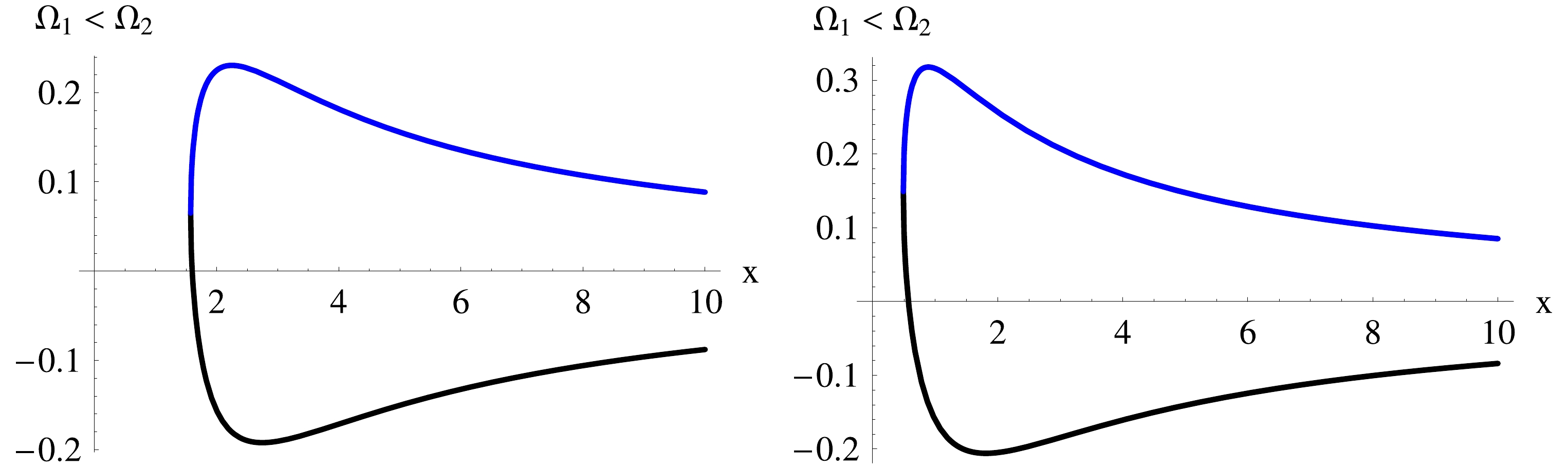
Figure 1. (color online) Plots of (
$ \Omega_1,\,\Omega_2 $ ) from Eq. (37) in units of$ 1/M $ . Shown are the dimensionless quantities ($ M\Omega_1,\,M\Omega_2 $ ) versus$ x = r/M $ , for$ \theta = \pi/2 $ and$ \alpha = 1/5 $ . In the left panel,$ b = 2\;\&\;c = 3 $ (analogous to KNBH with$ \epsilon^2 = 12/25 $ and$ \mu^2 = 0 $ ) , and in the right panel$ b = c = 7 $ ($ \epsilon^2 = \mu^2 = 45/98 $ ). The two curves meet at$ x = x_{\rm{h}} $ .We investigate the behavior of the norm of the vector
$ \vec{\Omega}_p $ ,$ |\vec{\Omega}_p| = \frac{\sqrt{\bar{g}_{11}\Omega_r^2+\bar{g}_{22}\Omega_\theta^2}}{2\sqrt{|\bar{g}|}\; \big|\bar{g}_{44}+2\Omega\bar{g}_{34}+\Omega^2\bar{g}_{33}\big|}, $

(38) where the presence of the metric coefficients (
$ \bar{g}_{11} = \rho^2/\Delta,\,\bar{g}_{22} = \rho^2 $ ) takes into account the fact that ($ \partial_r,\,\partial_{\theta} $ ) from Eq. (32) are not unit vectors. For the metric Eq. (12), ($ \Omega_\theta,\,\Omega_r $ ) are given by$ \begin{split} \Omega_\theta =& \frac{1}{H_3^2\rho^4}\Big\{2H_3^2H_4(r -m) - \frac{a\sqrt{bc}(4+bc)H_3^3m\sin^2\theta}{2(b+c)}+\Omega\Big[4rH_3H_4^2 -4mH_3H_4^2 -\frac{a\sqrt{bc}(4+bc)H_3^3 H_4m\sin^2\theta}{b+c} \\ &+2H_3^2(r-m)\rho^4\sin^2\theta+ H_3^2[H_2((b-2)m+2r)+H_1((-2+c)m+2r)]\Delta \sin^2\theta+4mH_3\rho^4\Delta\sin^2\theta -4rH_3\rho^4\Delta\sin^2\theta \Big]\\& +\Omega^2\Big[H_3H_4\rho^2\Big( 2(r-m)\rho^2+\frac{[H_2((b-2)m+2r)+H_1((c-2)m+2r)]\Delta}{\rho^2} \Big)\sin^2\theta - \frac{a\sqrt{bc}(4+bc)H_3H_4^2m\sin^2\theta}{2(b+c)}\\& -\frac{a\sqrt{bc}(4+bc)mH_3\rho^4\sin^2\theta}{2(b+c)} +2H_4(r-m)(H_4^2-\rho^4\Delta\sin^2\theta) \Big] \Big\}, \end{split} $

(39) $ \begin{split} \Omega_r = & \frac{1}{H_3^2\rho^4}\Big\{ \frac{a\sqrt{bc}H_3^3m[(b-2)(c-2)m-(4+bc)r]\cos\theta\sin\theta}{b+c}-2a^2H_3^2H_4\cos\theta\sin\theta \\ &+\Omega\Big[ \frac{2a\sqrt{bc}H_3^2H_4m[(b-2)(c-2)m-(4+bc)r]\cos\theta\sin\theta}{b+c}-2a^2H_3H_4^2\cos\theta\sin\theta +4a^2H_3\rho^4\Delta\cos\theta\sin^3\theta\\&\times \frac{aH_3^2\Delta\big[H_1[\sqrt{b^2-4}c\sqrt{c^2-4}m+4a(b+c)\cos\theta]+H_2[-b\sqrt{(b^2-4)(c^2-4)}m+4a(b+c)\cos\theta]\big]\sin^3\theta}{2(b+c)} \\ &+H_3^2\rho^4\Delta \sin(2\theta) \Big] +\Omega^2\Big[ \frac{a\sqrt{bc}H_3H_4^2m[(b-2)(c-2)m-(4+bc)r]\cos\theta\sin\theta}{b+c}\\ &+ \frac{a\sqrt{bc}H_3m((b-2)(c-2)m-(4+bc)r)\rho^2\cos\theta\sin^3\theta}{b+c} -2a^2H_4\cos\theta\sin\theta(H_4^2-\rho^4\Delta\sin^2\theta) +2H_3H_4\rho^2\Delta\sin\theta\\& \times \Big( \rho^2\cos\theta-\frac{a[H_1(\sqrt{(b^2-4)(c^2-4)}mc+4a(b+c)\cos\theta)+H_2(-b\sqrt{(b^2-4)(c^2-4)}m+4a(b+c)\cos\theta)]\sin^2\theta}{4(b+c)\rho^2} \Big)\Big] \Big\}, \end{split} $

(40) while the expression in the denominator of Eq. (38),
$ 2\sqrt{|\bar{g}|}\; \big|\bar{g}_{44}+2\Omega\bar{g}_{34}+\Omega^2\bar{g}_{33}\big| $ , simplifies to$ \frac{2\big|H_3^2+2\Omega H_3 H_4+\Omega^2(H_4^2-\rho^4\sin^2\theta\Delta)\big|\sin\theta}{|H_3|}. $

(41) For constant
$ \Omega $ , the zeros of Eq. (41) are denoted as$ x_1 $ and$ x_2 $ :$ \begin{array}{l} x_{\rm{h}}<x_1<x_{\rm{erg}}<x_2\quad{\rm{if}}\quad\Omega\neq\omega_h,\\ x_{\rm{h}} = x_1<x_{\rm{erg}}<x_2\quad{\rm{if}}\quad\Omega = \omega_h, \end{array} $

(42) where
$ \omega_h\equiv\omega(x = x_h) $ and$ \omega(x)\equiv -\bar{g}_{34}/\bar{g}_{33} $ is the ZAMO angular velocity satisfying$ \begin{split} \omega = -\frac{H_3H_4}{H_4^2-\rho^4\Delta\sin^2\theta}, \qquad \Omega_{1}\Omega_{2} = -\frac{H_3\omega}{H_4},\qquad M\omega_h = -M\frac{H_3}{H_4}\Big|_{x = x_h} = \frac{(b+c)^3\alpha}{2\sqrt{bc}[(bc+4)(b+c)x_h-4(b-2)(c-2)]}.\end{split} $

(43) A series expansion of
$ |\vec{\Omega}_p| $ for$ \alpha^2\ll 1 $ ,$ \epsilon^2\ll 1 $ ,$ \mu^2\ll 1 $ and$ \theta = \pi/2 $ yields$ \begin{split} |\vec{\Omega}_p| =& \bigg|\frac{\Omega(r-3 M) }{r-2 M-r^3 \Omega ^2}\bigg|\; \bigg\{1+\frac{M^2 \left(3 r^2 \Omega ^2-1\right) \left(2 M-r-r^3 \Omega ^2\right)}{r^2(3 M-r) \left(2 M-r+r^3 \Omega ^2\right) \Omega }\; \alpha\\ & +\frac{M^2 \left[12 M^3 \Omega ^2 r+\Omega ^2 \left(r^2 \Omega ^2-1\right) r^4+M \left(2-r^2 \Omega ^2+r^4 \Omega ^4\right) r-2 M^2 \left(2-2 r^2 \Omega ^2+9 r^4 \Omega ^4\right)\right]}{r (3 M-r) \left(2 M-r+r^3 \Omega ^2\right)^2}\; \alpha ^2\\ & -\frac{M (2 M^2-3 M r+13 M \Omega ^2 r^3-2 \Omega ^2 r^4)}{2 r (3 M-r) (2 M-r+r^3 \Omega ^2)}\; (\epsilon ^2+\mu ^2)+\cdots\bigg\},\quad \Omega\neq 0, \end{split}$

(44) $ |\vec{\Omega}_p| = \bigg|\frac{M^2 \alpha}{r^2 (r-2 M)}\bigg|\; \bigg\{1+\frac{M (6 M-5 r)}{2 r (r-2 M)}\; (\epsilon ^2+\mu ^2)+\cdots\bigg\},\; \Omega = 0. $

(45) These expressions were derived using Eq. (24). In the case
$ \Omega\neq 0 $ , even if BH is not rotating ($ \alpha = 0 $ ), there is a nonvanishing contribution to$ |\vec{\Omega}_p| $ as can be seen from Eq. (44), which for the Schwarzschild BH reduces to$ |\vec{\Omega}_p| = \bigg|\frac{\Omega(r-3 M) }{r-2 M-r^3 \Omega ^2}\bigg|, $

(46) In the Schwarzschild spacetime, it is known that if the gyroscope moves along a circular geodesic then its angular velocity, or Kepler frequency
$ \Omega = \Omega_{\rm{Kep}} $ , is related to the radius of the circle by$ \Omega\equiv\Omega_{\rm{Kep}} = \sqrt{M/r^3} $ . Replacing$ \Omega $ by$ \sqrt{M/r^3} $ in Eq. (46), we obtain$ |\vec\Omega_p| = \Omega_{\rm{Kep}} = \sqrt{M/r^3} $ , that is, the precession frequency is the same as the Kepler frequency. If in the Schwarzschild spacetime the gyroscope, supported by an engine, rotates with an angular velocity$ \Omega\neq\Omega_{\rm{Kep}} $ , then$ |\vec\Omega_p|\neq\Omega $ . Now, if the gyroscope has no angular velocity in the stationary spacetime,$ \Omega = 0 $ ($ K = \partial_t $ ), although the main contribution to$ |\vec{\Omega}_p| $ comes from rotation as can be seen from Eq. (45), there are contributions from the electric ($ \epsilon^2 $ ) and magnetic ($ \mu^2 $ ) charges as well.Let us go back to the general expression Eq. (38). For
$ \Omega = 0 $ , there is nothing particular in this case as shown in Fig. 2: the gyroscope remains on a timelike curve for all$ x>x_{\rm{erg}} $ . As the black hole becomes more charged, the three-space outside the ergo-region extends. For$ \Omega\neq 0 $ , as shown in the right panel of Fig. 2 where$ \Omega = 1/10 $ , the norm$ |\vec{\Omega}_p| $ diverges at the two zeros$ x_1 $ and$ x_2 $ of the denominator of Eq. (38), given in Eq. (41), and for$ \Omega $ constant, the gyroscope remains on a timelike curve only for$ x $ between these zeros. As the black hole becomes more charged, both zeros decrease and the three-space between them extends.
Figure 2. (color online) Plots of
$ |\vec{\Omega}_p| $ from Eq. (38) in units of$ 1/M $ . Shown is the dimensionless quantity$ M|\vec{\Omega}_p| $ versus$ x = r/M $ for$ \theta = \pi/2 $ and$ \alpha = 1/5 $ . Blue lines correspond to$ b = c = 7 $ ($ \epsilon^2 = \mu^2 = 45/98 $ ), red lines to$ b = c = 3 $ and ($ \epsilon^2 = \mu^2 = 5/18 $ ), magenta lines to$ b = 2\;\&\;c = 3 $ (analogous to KNBH with$ \epsilon^2 = 12/25 $ and$ \mu^2 = 0 $ ), and black lines to$ b = c = 2 $ corresponding to the Kerr black hole. In the left panel,$ \Omega = 0 $ . The norm$ |\vec{\Omega}_p| $ diverges on the surface of the ergo-region$ x = x_{\rm{erg}} $ and the gyroscope remains on a timelike curve for all$ x>x_{\rm{erg}} $ . As the black hole becomes more charged, the three-space outside the ergo-region extends. In the right panel,$ \Omega = 1/10 $ . The norm$ |\vec{\Omega}_p| $ diverges at the two zeros$ x_1 $ and$ x_2 $ of the denominator of Eq. (38), given in Eq. (41), and the gyroscope remains on a timelike curve only for$ x $ between these zeros. As the black hole becomes more charged, both zeros decrease and the three-space between them extends.Note the existence of a point
$ x_{\min} $ where$ |\vec{\Omega}_p(x_{\min})| = 0 $ , that is where$ \Omega_\theta(x_{\min}) = 0 $ and$ \Omega_r(x_{\min}) = 0 $ . Such a point may offer a way for distinguishing between KNBH and RKKBH. Another way to distinguish between these BHs is to consider the minimum value of$ M\Omega_1 $ and the maximum value of$ M\Omega_2 $ versus$ \epsilon^2 $ , as depicted in Fig. 1 and subsequent figures. -
The metric of KNBH may be brought to the form of Eq. (12) with
$\begin{split} \frac{\rho_{\rm{KN}}^2}{M^2} =& x^2+\alpha^2\cos^2\theta, \\ \frac{\Delta_{\rm{KN}}}{M^2} =& x^2-2x+\epsilon^2+\alpha^2, \end{split}$

(47) $\begin{split} \frac{H_{3\,({\rm{KN}})}}{M^2} =& x^2+\alpha^2\cos^2\theta-2x+\epsilon^2, \\ \frac{H_{4\,({\rm{KN}})}}{M^3} =& \alpha (2x-\epsilon^2)\sin^2\theta. \end{split}$

(48) We consider a KNBH and RKKBH with no magnetic charge (
$ \mu^2 = 0 $ ). In Fig. 3, we show the plot of$ x_{\min}(\epsilon^2) $ with$ |\vec{\Omega}_p(x_{\min})| = 0 $ . The event horizon$ x_{\rm{h}} $ versus$ \epsilon^2 $ is also shown. We are interested in the region outside the event horizon. For the numerical set used in Fig. 3, the values of$ x_{\min} $ range from 2 to 2.7. The range of electric charge for$ x_{\min}\geq x_{\rm{h}} $ is, however, much larger for RKKBH.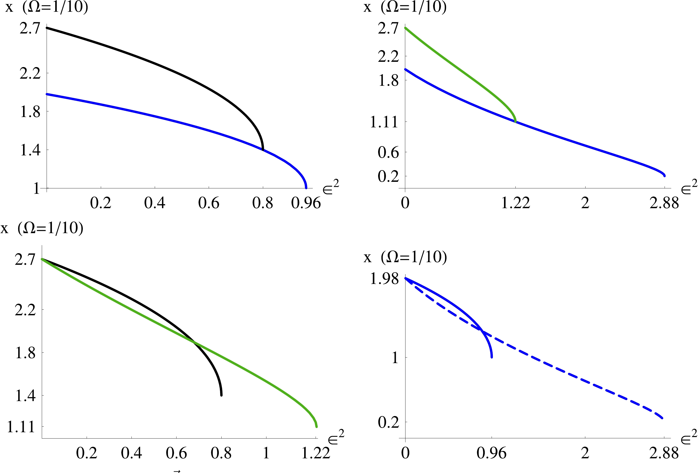
Figure 3. (color online) Plots of
$ x_{\min} $ with$ |\vec{\Omega}_p(x_{\min})| = 0 $ , the event horizon$ x_{\rm{h}} $ and the outer radius of the ergo-region, versus$ \epsilon^2 $ for$ \theta = \pi/2 $ ,$ \alpha = 1/5 $ and$ \Omega = 1/10 $ . Upper left panel: the black line represents$ x_{\min}(\epsilon^2) $ , and the blue line$ x_{\rm{h}}(\epsilon^2) $ for KNBH. The blue line ends at ($ 0.96,\,1 $ ) corresponding to the extremal KNBH. Upper right panel: the green line represents$ x_{\min}(\epsilon^2) $ , and the blue line$ x_{\rm{h}}(\epsilon^2) $ for RKKBH with no magnetic charge ($ \mu^2 = 0 $ ). The blue line ends at ($ 2.88,\,0.2 $ ) corresponding to the extremal RKKBH. Lower left panel: the black line represents$ x_{\min}(\epsilon^2) $ for KNBH, and the green line$ x_{\min}(\epsilon^2) $ for RKKBH. The plots are the same as in the upper left and upper right panels but without the horizon plots. In the upper left and upper right panels the curve$ x_{\min}(\epsilon^2) $ starts at 2.7 corresponding to the Kerr BH. Lower right panel: the continuous line represents the outer radius of the ergo-region of KNBH, and the dashed line the outer radius of the ergo-region of RKKBH. The plots are the same as in the upper left and upper right panels but without the$ x_{\min}(\epsilon^2) $ plots.We do not expect the charge of a black hole to exceed its mass, so we focus on the physical region corresponding to
$ \epsilon^2\ll 1 $ . In this case, as seen from the right panel of Fig. 3, a moving gyroscope following a timelike path with an angular velocity$ \Omega\neq 0 $ , may reveal the nature of BH. To be more precise, we provide the calculations for$ \epsilon^2 = 1/100 $ . This yields$ x_{\min} = 2.66275 $ for KNBH, and$ x_{\min} = 2.65781 $ for RKKBH, which do not depend on the mass of BH and correspond to$ \Delta x = 0.00493387 $ . Introducing the relevant physical constants, we obtain$ \Delta r = \frac{GM}{{\rm c}^2}\; \Delta x, $

(49) where
$ G = 6.673\times 10^{-11} $ and$ {\rm c} = 299792458 $ in SI units. For a BH with the solar mass ($ M_\odot = 1.9888\times 10^{30} $ kg),$ \Delta r = 7.3 $ m, and for a BH with one million solar masses,$ \Delta r = 7.3\times 10^{6} $ m. In terms of$ r $ , the gyroscope will not detect a spin precession, corresponding to a vanishing value of$ |\vec{\Omega}_p| $ at$ r_{\min} = 3.93188\times 10^{9} $ m , if it is moving along a timelike path in a KNBH. On the other hand, if$ |\vec{\Omega}_p| $ vanishes at some smaller value of$ r $ , such that$ \Delta r = 7.3\times 10^{6} $ m, then this corresponds to a RKKBH with no magnetic charge. -
Another way to distinguish KNBH from RKKBH is to compare the extrema of the dimensionless functions (
$ M\Omega_{1},\,M\Omega_{2} $ ) for both BHs. In Fig. 4, we show the maximum values of ($ M|\Omega_{1}|,\,M\Omega_{2} $ ) versus$ \epsilon^2 = Q^2/M^2 $ . For$ \epsilon^2 = 1/100 $ , we have$ M\Omega_{2(\max)} = 0.2094775 $ for KNBH , and$ M\Omega_{2(\max)} = 0.2094763 $ for RKKBH with$ \mu^2 = 0 $ . These values, which are independent of the mass$ M $ , show that for$ 0.2094763<M\Omega\leqslant 0.2094775 $ a gyroscope in the geometry of KNBH can still follow a prograde timelike path, while this is not possible in the geometry of RKKBH. For the same value of$ \epsilon^2 $ , we obtain$ M\Omega_{1(\min)} =-0.1792895775\simeq $ $ -0.1792896 $ for KNBH , and$ M\Omega_{1(\min)} = -0.1792890227\simeq $ $ -0.1792890 $ for RKKBH with$ \mu^2 = 0 $ . This shows that for$-0.1792896\leqslant M\Omega< $ $ -0.1792890 $ a gyroscope in the geometry of KNBH can still follow a retrograde timelike path while this is not possible in the geometry of RKKBH.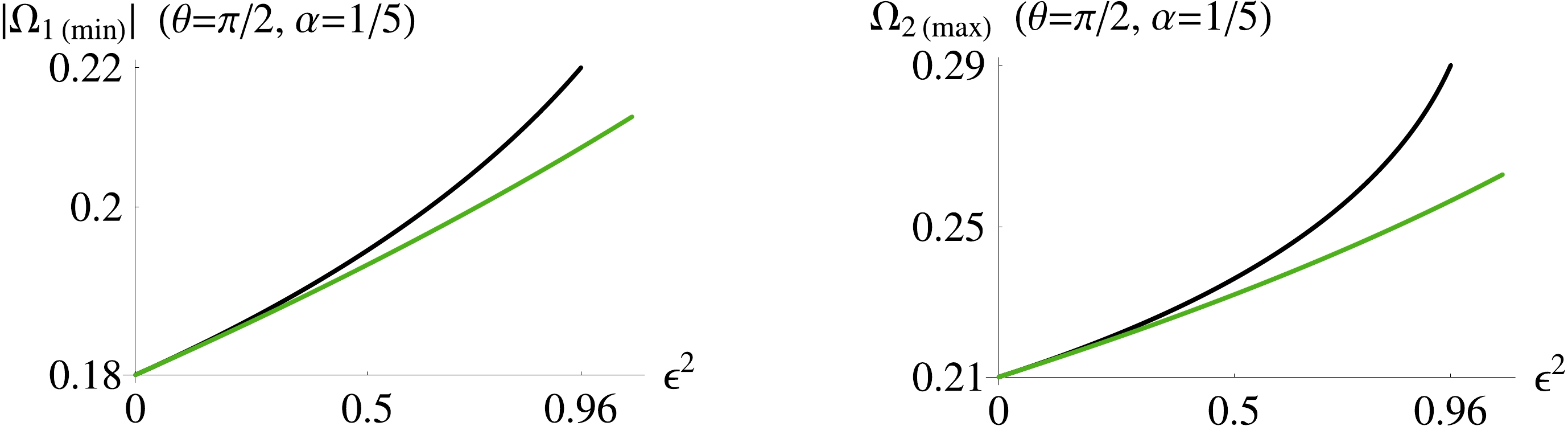
Figure 4. (color online) Left panel: absolute value of the minimum of
$ \Omega_1 $ from Eq. (37), in units of$ 1/M $ (plot of$ M|\Omega_{1(\min)}| $ ), versus$ \epsilon^2 = Q^2/M^2 $ for$ \theta = \pi/2 $ and$ \alpha = 1/5 $ . The black line is for KNBH, and the green line for RKKBH. Right panel: maximum of$ \Omega_2 $ from Eq. (37), in units of$ 1/M $ (plot of$ M\Omega_{2(\max)} $ ), versus$ \epsilon^2 $ for$ \theta = \pi/2 $ and$ \alpha = 1/5 $ . The black line is for KNBH, and the green line for RKKBH with$ \mu^2 = 0 $ . The green line extends to$ \epsilon^2 = 2.88 $ , the value of$ \epsilon^2 $ for an extremal RKKBH (Fig. 3).We have chosen
$ \epsilon^2 = 1/100 $ relatively small because we believe that most BHs are lightly charged. For this value of$ \epsilon^2 $ we see that$ M\min(\Omega_1(r,\theta)) $ and$ M\max(\Omega_2(r,\theta)) $ differ only in the seventh decimal. From an experimental point of view, it may be difficult but not impossible to perform such a measurement. However, as is clear from Fig. 4, had we chosen a higher value of$ \epsilon^2 $ ,$ M\min(\Omega_1(r,\theta)) $ and$ M\max(\Omega_2(r,\theta)) $ would have differed in a even lower decimal order. -
In this study, we have extended the analysis of the gyroscope precession frequency to five-dimensional charged rotating black holes in Kaluza-Klein theory. This phenomenon is related to a stationary gyroscope moving along a timelike curve in a stationary black hole spacetime. We derived a formula for the general precession frequency of the test gyroscope, valid for general five-dimensional rotating black holes, by dimensional reduction to four dimensions. From the empirical perspective, we studied the magnitude of the precession frequency vector associated with the test gyroscope in the KK spacetime
$ |\vec{\Omega}_p | $ , and the limiting frequencies for timelike motion ($ \Omega_{1},\,\Omega_{2} $ ). We showed that$ |\vec{\Omega}_p | $ may vanish if$ \Omega\neq 0 $ , and that this fact can be used to distinguish between astrophysical black holes. We also showed how the extreme values of ($ \Omega_{1},\,\Omega_{2} $ ) may help to distinguish between astrophysical black holes. Both schemes are mass independent.There are few important points to note:
$ |\vec{\Omega}_p | $ diverges at two spatial locations outside the event horizon, enclosing the outer radius of the ergo-region. However, if$ \Omega = 0 $ , than the norm$ |\vec{\Omega}_p | $ diverges at a single location only, which is the outer radius of the ergo-region. Moreover, the angular speed$ \Omega $ of the stationary gryoscopes takes both positive and negative values, meaning that the gyroscopes move around the black hole in prograde and retrograde orbits, respectively. The maximum of$ \Omega_2 $ occurs much closer to the horizon compared to the minimum of$ \Omega_1 $ . Ultimately, as the gyroscope approaches the horizon, both$ \Omega_1 $ and$ \Omega_2 $ approach the ZAMO angular velocity.The extra dimension is an important concept in modern gravity theory and there is no experiment to prove or disprove this hypothesis. In our work, we found that a rotating KK black hole is always different from a Kerr-Newman black hole, which implies that the hypothesis of extra dimension can be tested by an analysis of the gyroscope precession frequency. Recall that the hypothesis of KK asserts that the extra dimension is compactified throughout the whole spacetime and, consequently, the 4+1 decomposition remains valid for the whole range of coordinates. The construction of KKBHs is entirely based on this hypothesis. This implicitly assumes that the gravitational field, particularly near and outside the outer radius of the ergo-region, is not strong enough to allow probing the extra dimension.
On the other hand, it is thought that the graviton can play an important role in investigating extra dimensions, and that gravitational perturbation could include critical information about the properties of spacetime with extra dimensions. We plan to study the gravitational perturbation effect on the gyroscope precession in a subsequent work.
-
The four-velocity of an observer at rest along an integral curve
$ \gamma $ of$ K $ is$ \tag{A1} u = \frac{K}{\sqrt{|K^2|}}. $

(A1) Let
$ e_4 = u $ and$ e_i $ ($ i $ :$ 1\to 3 $ ) form an orthonormal tetrad:$ <e_\mu,e_\nu> = \eta_{\mu\nu} $ [($ \mu,\nu $ ):$ 1\to 4 $ ] where$ \eta_{\mu\nu} = {\rm diag}(-1,1,1,1) $ and$ <,> $ denotes the scalar product. As time evolves, we want the three elements of the triad$ e_i $ to remain perpendicular to each other and to$ u\propto K $ . The only transport along$ \gamma $ that preserves orthogonality is the Lie derivative. Thus, we choose the triad$ e_i $ such that$ L_K e_i = 0 $ . Along with$ L_K e_{4}\propto L_K K\equiv 0 $ , which is identically satisfied, we can write$ \tag{A2} L_K e_{\mu} = 0. $

(A2) This is the Copernican system [47]. In other words, the basis vectors
$ e_{i} $ are tied to an inertial system far from the source (BH) and fixed relative to distant stars [48].The spin
$ S $ of the gyroscope obeys the equation [47,48]$ \tag{A3} \nabla_u S = <S,\nabla_u u>u\;{\rm{with}}\;<S,u> = 0, $

(A3) where
$ \nabla_u u $ is the acceleration of the gyroscope along an integral curve$ \gamma $ of$ K $ . This acceleration is generally nonzero. As$ <S,u> = 0 $ ,$ S $ is a purely spatial vector,$ S^4 = 0 $ and$ S = S^ie_i $ . Evaluating$ {\rm d}S^i/{\rm d}\tau = \nabla_u <e^i,S> $ where$ e^{\mu} = \eta^{\mu\nu}e_{\nu} $ ($ e^{i} = e_{i} $ ), results in$ \tag{A4} \frac{{\rm d}S^i}{{\rm d}\tau} = S^j <\nabla_u e_i,e_j> = S^j \omega_{ij}\quad{\rm{with}}\quad\omega_{ij}: = <\nabla_u e_i,e_j>. $

(A4) Here, we have dropped the term
$ <e_i,\nabla_u S> $ which is zero due to Eq. (A3). Since$ <e_i,e_j> = \eta_{ij} $ ,$ \omega_{ij} $ is anti-symmetric:$ \omega_{ij} = -\omega_{ji} $ . Thus, the right-hand side of Eq. (A4) can be written in the form$ \varepsilon_{ijk}S^j\Omega^k $ , where$ \vec{\Omega}_p = \Omega^k e_k $ is the spin angular velocity of precession in the Copernican system defined above. It is related to$ \omega_{ij} $ by$ \tag{A5} \omega_{ij} = \varepsilon_{ijk}\Omega^k, $

(A5) where
$ \varepsilon_{ijk} $ is the totally anti-symmetric symbol. Using the property$ \varepsilon^{ijl}\varepsilon_{ijk} = 2\delta^l_k $ $ \tag{A6} \Omega^l = \frac{\varepsilon^{ijl}\omega_{ij}}{2} = \frac{\varepsilon^{ijl}<\nabla_u e_i,e_j>}{2} = \frac{\varepsilon^{ijl}<\nabla_K e_i,e_j>}{2\sqrt{|K^2|}}. $

(A6) From the symmetry of the connection,
$ \Gamma^{\sigma}_{\mu\nu} = \Gamma^{\sigma}_{\nu\mu} $ , it follows that$ \nabla_K e_i-\nabla_{e_i} K = [K,e_i] $ . For any vector field belonging to the class$ C^{\infty} $ , we have$ L_X Y = [X,Y] $ , which results in$ \nabla_K e_i-\nabla_{e_i} K = [K,e_i] = L_K e_i = 0 $ due to Eq. (A2), and thus$ \nabla_K e_i = \nabla_{e_i} K $ , so that Eq. (A6) transforms to$ \tag{A7} \omega_{ij} = \frac{<\nabla_{e_i} K,e_j>}{\sqrt{|K^2|}},\qquad\Omega^l = \frac{\varepsilon^{ijl}<\nabla_{e_i} K,e_j>}{2\sqrt{|K^2|}}. $

(A7) Since
$ <K,e_j> = 0 $ , we have$ <\nabla_{e_i} K,e_j> = -<K,\nabla_{e_i} e_j> $ . Recalling that$ \omega_{ij} $ is anti-symmetric, Eq. (A7) results in$ \tag{A8} \omega_{ij} = \frac{<K,\nabla_{e_j} e_i-\nabla_{e_i} e_j>}{2\sqrt{|K^2|}} = -\frac{<K,[e_i,e_j]>}{2\sqrt{|K^2|}} = -\frac{\bar{K}([e_i,e_j])}{2\sqrt{|K^2|}}, $

(A8) where
$ \bar{K} $ is the one-form of$ K $ . Using the result from differential geometry:$ {\rm d}\omega(X,Y) = X\omega(Y)-Y\omega(X)-\omega([X,Y]), $

where
$ X $ and$ Y $ are vector fields and$ \omega $ is a one-form. Let$ \omega = \bar{K} $ ,$ X = e_i $ and$ Y = e_j $ , then we have$ \bar{K}([e_i,e_j]) = -{\rm d}\bar{K}(e_i,e_j) $ and the other two terms vanish:$ \bar{K}(e_i) = [K,e_i] = L_K e_i = 0 $ . Finally$ \tag{A9} \omega_{ij} = \frac{1}{2\sqrt{|K^2|}}\; {\rm d}\bar{K}(e_i,e_j). $

(A9) This equation was derived in [47] using a similar analysis to the one presented here. It is straightforward to convert this equation to the one-form
$ \bar{\Omega}_{p} $ of$ \vec{\Omega}_p = \Omega^ke_k = (\varepsilon^{ijk}\omega_{ij}/2)e_k $ , as shown in [47]$ \tag{A10} \bar{\Omega}_{p} = \frac{1}{2K^{2}}\ast ( \bar{K}\wedge {\rm d}\bar{K}), $

(A10) which is equation Eq. (31).
Gyroscope precession frequency analysis of a five-dimensional charged rotating Kaluza-Klein black hole
- Received Date: 2019-11-01
- Accepted Date: 2020-01-18
- Available Online: 2020-06-01
Abstract: We study the spin precession frequency of a test gyroscope attached to a stationary observer in the five-dimensional rotating Kaluza-Klein black hole (RKKBH). We derive the conditions under which the test gyroscope moves along a timelike trajectory in this geometry, and the regions where the spin precession frequency diverges. The magnitude of the gyroscope precession frequency around the KK black hole diverges at two spatial locations outside the event horizon. However, in the static case, the behavior of the Lense-Thirring frequency of a gyroscope around the KK black hole is similar to the ordinary Schwarzschild black hole. Since a rotating Kaluza-Klein black hole is a generalization of the Kerr-Newman black hole, we present two mass-independent schemes to distinguish these two spacetimes.


 DownLoad: