


 Abstract
 HTML
HTML Reference
 Related
 PDF
PDF


-
The rapid development of computational resources, i.e., GPU, deep learning has achieved remarkable progress in numerous fields, such as object detection and classification [1–3], machine translation [4,5] and speech recognition [6–8]. While traditional methods often resolve these issues through handcrafted features based on expertise knowledge, deep learning methods learn the internal representation through an end-to-end training paradigm, i.e., convolutional neural networks (CNNs) [9,10] and recurrent neural networks (RNNs) [11–13]. The characteristics of sparse connectivity and parameter sharing make the CNN a powerful engine in analyzing image data, while internal units with loops and states make the RNN efficient for modeling time-dependent series.
The success of these deep learning methods is partially owed to their effectiveness in extracting the latent representation from regular Euclidean data (i.e., image, text, speech). Presently, there is an increasing number of demands for effectively analyzing non-Euclidean data with irregular and complex structures. Proposed methods construct this data as graph-structured data and exploit the deep learning to learn their representation. For example, in e-commerce and social media platforms, the graph-based learning system exploits interactions between users and products to make highly accurate recommendations [14,15]. In chemistry, the molecules are modeled as graphs to explore and identify their chemical properties [16]. In the high-energy physics field, researchers need to analyze a large amount of irregular signals. Consequently, studies seek to improve the analysis efficiency with graph neural networks (GNNs). Impressive progress has been achieved, including improvement of the neutrino detecting efficiency on the IceCube [17], exploring SUSY particles [18], and recognizing jet pileup structures [19] on the LHC.
Precise measurement of the cosmic-ray (CR) spectrum and its components at the PeV scale is essential to probe the CR origin, acceleration, and propagation mechanisms, as well as to explore new physics. A spectral break at ~ 4 PeV, referred to as the CR knee, was discovered 60 years ago [20]; however, its origin remains a mystery. Precise localization of the knees of different chemical compositions is key to explore the hidden physics. Current explanations of the CR knee can be classified into two categories with different mechanisms, including the mass-dependent knee and rigidity-dependent knee models [21], where models with the rigidity-dependent knee are often considered to originate from the acceleration limit and the galactic leakage mechanism, and many of these models with a mass-dependent knee are associated with new physics. This new physics involves exploring a new interaction channel and dark matter, as summarized in Ref. [21]. Although extensive efforts were made aiming at resolving this issue, the experimental measurements exhibit large discrepancies between each other [22–25].
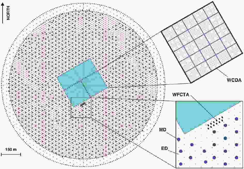
The Large High Altitude Air Shower Observatory (LHAASO) performs next-generation CR experiments [26], which aim to precisely measure the CR spectrum along with light groups from 10 TeV to EeV and survey the northern hemisphere to identify gamma-ray sources with a high sensitivity of 1% Crab units. The observatory is located at a high altitude (4410 m a.s.l.) in the Daocheng site, Sichuan Province, China. It consists of an EAS array (KM2A) covering 1.3 km2 area, a 78000 m2 closed packed water Cherenkov detector array (WCDA), and 12 wide-field Cherenkov/fluorescence telescopes (WFCTA). The LHAASO-KM2A occupies most of the area and is composed of two sub-arrays, including a 1.3 km2 array of 5195 electromagnetic particle detectors (ED) and the overlapping 1
$ {\rm km}^2 $ array of 1171 underground water Cherenkov tanks as muon detectors (MD). The WCDA contains three water ponds with the effective depth of about 4 m. Each pond is divided into 5 × 5 m2 cells with an 8-inch PMT located at the bottom to observe the Cherenkov light generated by the EAS secondary particles in the water. The focal plane camera in each telescope of WFCTA has 32 × 32 pixels with a size$ 0.5^{\circ} \ \times \ 0.5^{\circ} $ of each.The layout of each component of LHAASO is illustrated in Fig. 1, where the red and blue points represent KM2A-ED and KM2A-MD detectors, respectively. The ED detectors are divided into two parts, the central part with 4901 detectors and an out-skirt ring with 294 detectors to discriminate showers with their core located within the central area from the outside ones. An ED unit consists of four plastic scintillation tiles (100 × 25 × 1 cm3 each) covered by 5 mm thick lead plates to absorb the low-energy charged particles in showers and convert the shower photons into electron-positron pairs. The MD array plays the key role in discriminating the gamma-rays from the CR nuclei background, and it offers important information for classifying CR groups. An MD unit has an area of 36 m2, buried by the overburden soil with 2.5 m height for shielding the electromagnetic components in showers. It is designed as a Cherenkov detector underneath the soil, to collect the Cherenkov light induced by muon parts when they penetrate the water tank.
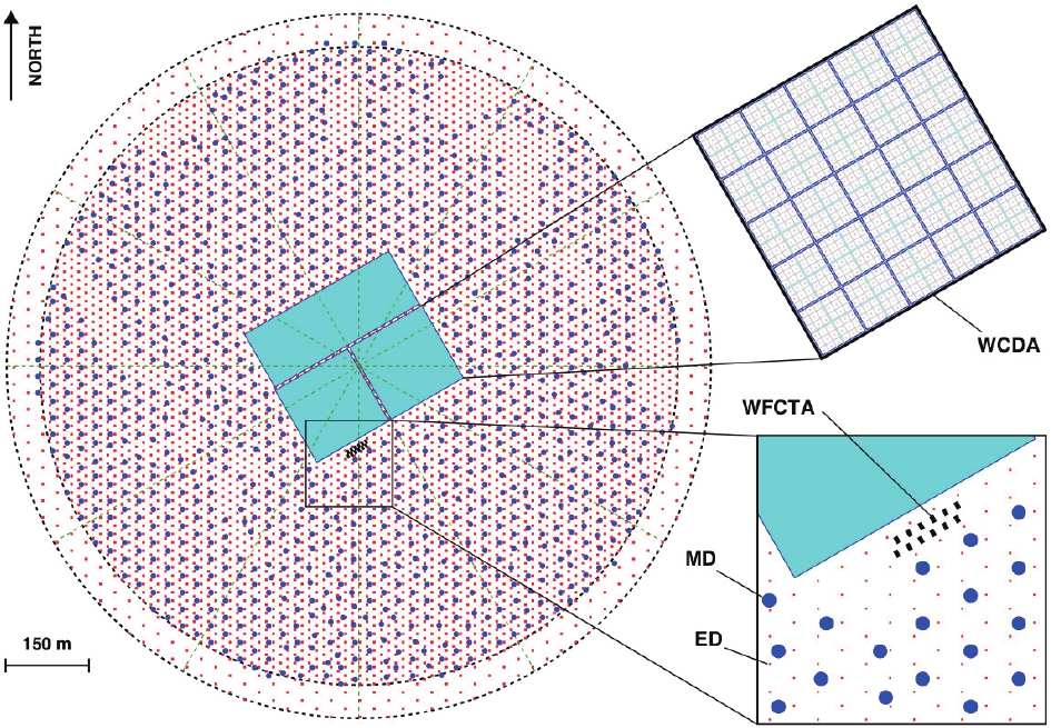
Figure 1. (color online) Layout of LHAASO experiment. Insets show details of one pond of WCDA, and EDs (red points) and MDs (blue points) of KM2A. WFCTA, located at WCDA edge, are also shown.
Several studies addressed the component discrimination of the LHAASO hybrid detection using both expertise features [27] and machine learning methods [28]. These hybrid detection methods utilize the effective information offered by entire LHAASO arrays. Although they exhibit a remarkable performance, their statistics are limited due to the poor operation time and aperture. Under the merit of the large area, full duty cycle, and excellent
$ \gamma / P $ discrimination ability, the LHAASO-KM2A is an ideal candidate for studying the CR component classification task. In this study, we leverage the GNN to improve the CR-component classification performance in the LHAASO-KM2A experiment, where the detector activated by the event is formed asgraph-structured data. Our previous study [21] showed that the issue requires high accuracy in classifying the CR Proton (P task) and Light-component (L task) from the background. Hence, we focus on these two tasks. To evaluate the GNN performance, we introduce the traditional physics-based method with the handcrafted feature as the baseline. The subsequent sections are organized as follows. First, we introduce the physics baseline method in Section 2. Then, we review the development of the GNN framework and propose our KM2A GNN framework in Section 3. We perform the experiment and evaluate the results in Section 4 and Section 5. In the last Section, we provide a conclusion regarding GNN performance. -
Current experiments detect high-energy CRs completely via indirect methods, which measure the secondary particles of the extensive air showers (EAS) induced by the primary CR nuclei. The shower-to-shower fluctuations make classification of CR primaries difficult. When the CR nuclei impinge on top of the atmosphere, they suffer hadronic interaction with air molecules and generate daughter particles recursively. This is referred to as the hadron cascade. The sequence of this interaction proceeds by the following reaction and decay schemes [29]
$ \begin{array}{*{20}{l}} {p + p}&{ \to N + N + {n_1}{\pi ^ \pm } + {n_2}{\pi ^0}}\\ {{\pi ^0}}&{ \to 2\gamma }\\ {{\pi ^ + }}&{ \to {\mu ^ + } + {\nu _\mu }\;({\rm charge\;conjugate},\;c.c.)}\\ {{\mu ^ + }}&{ \to {e^ + } + {{\bar \nu }_\mu } + {\nu _e}\;(c.c.)} \end{array}$

Here, the photons, electrons, and positrons form most electromagnetic parts of the EAS and in turn generate themselves through the pair-production
$ \gamma \rightarrow e^+ + e^- $ and the bremsstrahlung process$ e^{\pm} \rightarrow e^{\pm} + \gamma $ , which is referred to as the electromagnetic cascade. Neutrinos form the missing part of the EAS, which is generally ignored in experiments. The muons do not form a cascade themselves and have a relatively long life (2.2$ \mu $ s) and comparatively small energy loss in the media, such that a large fraction of muons produced in a shower will penetrate the atmosphere and accumulate until their arrival at the observation level.The task of classifying CR primary groups relies on the electromagnetic and muon parts of the EAS. In the first-order approximation [30], a primary CR nucleus with mass A and energy E can be regarded as a swarm of A independent nucleons generating A superimposed proton-induced hadron cascades with energy
$ E/A $ . Because the heavier CR nucleus has less energy for each nucleon, it can interact with the air molecules at higher altitude. Hence, their shower electromagnetic components will suffer more attenuation with longer interaction length, and$ \pi^{\pm} $ components will have more opportunity to decay into muon parts. Consequently, the ratio of the electromagnetic to muon parts is a component-sensitive estimator, and it is adopted widely in CR experiments [25].Because the LHAASO-KM2A array can discriminate the electron and muon parts in the shower by ED and MD arrays, we formulate the ratio of collected signals from the MD and ED
$ N_{\mu} / N_e $ as the physics-based baseline model.$ N_{\mu} $ and$ N_e $ denote the collected photoelectrons of an event recorded by activated MD and ED detectors, respectively. The selection criterion is optimized, where the active ED detectors are counted within the distance 100 m from the shower core, and the active MD detectors are counted within 40 ~ 200 m. The occlusion area within 40 m of the MD serves to eliminate the punch-through effect, where the high-energy electronic particles near the shower core can penetrate the soil-shielding layer and fire the beneath MD detectors. We illustrate the distribution of the ratio$ N_{\mu} / N_e $ with respect to CR components and energies in Fig. 2, based on the simulation in Section 4. As shown, the heavier components exhibit larger values of$ N_{\mu} / N_e $ , while the proton lies at the bottom.
Figure 2. (color online) Distribution of
$N_{\mu} / N_e$ for each CR group (P (red), He (violet), CNO (blue), MgAlSi (yellow), Fe (green)) across energies from 100 TeV to 10 PeV. -
GNN architectures are specialized to effectively analyze graph-structured data. Many of them adopt the concept from convolution networks and design their graph convolution operations. In comparison with different graph convolution schemes, most GNN models are classified into two categories, including the spectral and spatial domains [31]. The spectral methods are formulated based on the graph signal processing theory [32,33], where the graph convolution is interpreted as filtering the graph signal on a set of weighted Fourier basis functions. Spatial methods explicitly aggregate the information from the neighbor through the weighted edges.
Suppose an undirected, connected, weighted graph is denoted as
$ G = \{ V, E, A\} $ , which consists of a set of vertices$ V $ , a set of edges$ E $ , and a weighted adjacency matrix$ A $ . The spectral-based approach is defined based on the normalized graph Laplacian, defined as$ L = I - D^{-1/2}AD^{-1/2} $ , where$ D $ is the diagonal matrix of$ G $ . Because the Laplacian$ L $ is a real symmetric positive semidefinite matrix, it can be factored as$ L = U \Lambda U^T $ through the eigenvalue decomposition algorithm. Hence, the Fourier basis$ F(x) = U^T x $ can be used for the graph filtering, and the spectral graph convolution operation is further simplified as$ \begin{array}{l} x * G \ g_{\theta} = U g_{\theta} U^T x , \end{array} $

(1) where
$ g_{\theta} = {\rm diag}(U^T g) $ is the learnable filter.Bruna et al. [34] proposed the first spectral convolution neural network (spectral CNN), with the spectral filter
$ g_{\theta} = \Theta^k_{i,j} $ as a set of learnable parameters. Because of the high computation complexity of the Fourier basis U, Defferrard et al. [35] proposed the Chebyshev spectral CNN (ChebNet) by introducing Chebyshov polinomials as the filter, i.e.,$ g_{\theta} = \sum^K_{i = 1} \theta_i T_k(\tilde{\Lambda}) $ , where$ \tilde{\Lambda} = 2\Lambda / \lambda_{\max} - I_N $ . Consequently, the ChebNet can avoid computation of the graph Fourier basis and significantly reduce computation complexity. Furthermore, Kipf et al. [36] simplified the ChebNet as a first-order approximation by assuming the$ K = 1 $ and$ \lambda_{\max} = 2 $ . The resulting graph convolution is located entirely in the spatial domain.The spatial-based graph convolution is defined based on the node's spatial relations. Following the idea of "correlation with template", the graph convolution relies on employing the local system at each node to extract the patches. Masci et al. [37] introduced the geodesic CNN (GCNN) framework, which generalizes the CNN into the non-Euclidean manifolds. Boscaini et al. [38] considered it as the anisotropic diffusion process. Monti et al. [39] generalized those spatial-domain networks and proposed mixture model networks (MoNet), a generic framework deep learning in the non-Euclidean domains. In this framework, a spatial convolution layer is given by a template-matching procedure as
$ \begin{array}{l} (f * g)(x) = \displaystyle\sum\limits^{J}_{j = 1} g_j D_j(x) f . \end{array} $

(2) The patch operator in Eq. (2) assumes the form
$ \begin{array}{l} D_j(x)f = \displaystyle\sum\limits_{y \in N(x)} \omega_j(u(x,y))f(y), j = 1, \cdots, J \ , \end{array} $

(3) where J represents the dimension of the extracted graph;
$ x $ denotes a point in the graph or the manifold, and$ y \in N(x) $ represents the neighbors of$ x $ .$ u(x,y) $ associates the node with the pseudo coordinate, and$ \omega_j(u) $ is the weighting function parameterized by learnable parameters.The definition of the patch operator associates MoNet with other spatial-based graph convolutional models through the choice of the pseudo coordinate
$ u(x,y) $ and the weighting function$ \omega_j(u(x,y)) $ . Consequently, those spatial-based methods can be considered as particular instances of the MoNet. In particular, a convenient choice of the weighting function is the Gaussian kernel$ \begin{array}{l} \omega_j(u) = \exp \left(-\frac12 (u - \mu_j)^T \Sigma^{-1}_j (u - \mu_j)\right), \end{array} $

(4) where
$ \Sigma_j $ and$ \mu_j $ are the learnable$ d \times d $ and$ d \times 1 $ covariance matrix and mean vector of a Gaussian kernel, respectively.Spectral-based methods have their mathematical foundations in the graph signal processing; however, high computational costs are involved in calculating the Fourier transform. Spatial-based methods are intuitive by directly aggregating information from the neighbors, and they have the potential to handle large graphs. In contrast, as the Laplacian-based representation is required for spectral convolution, a learned model cannot be applied on another different graph, while the spatial-based convolution can be shared across different locations and structures. Because the CR EAS event changes its location, direction, and energy, the spatial-domain method is suitable to analyze the LHAASO-KM2A experiment.
-
LHAASO-KM2A detectors can record the arrival time and photoelectron amplitude of shower secondary particles. The distribution of detector photonelectrons with respect to the distance from the shower core roughly obeys the NKG function [40,41] with the most dense region located at the shower core, while the distribution of arrival times can be parameterized as a plane perpendicular to the direction of the shower. Accordingly, we perform the data preprocessing procedure by reconstructing the event to locate the shower core position (
$ x_0 $ ,$ y_0 $ ) and direction ($ \theta_0 $ ,$ \phi_0 $ ). The photoelectrons are normalized to the reconstructed event energy for an energy-invariant representation, denoted as$ pe $ . Because the shower geometry is often treated as a slanted symmetric plane around the shower core, we transform the detector positions ($ x_i $ ,$ y_i $ ) into the cylinder coordinate ($ r_i $ ,$ \phi_i $ ) with the zero point at the shower core. The shower event along the time axis is represented by the detector's time residual$ {d}T_i $ , defined as$ \begin{array}{l} {d}T_i = T_i - \dfrac{{{ r}_i} \cdot {{ r}_0}}{c \lVert {{ r}_0} \rVert} - T_0 ,\end{array} $

(5) where
$ T_i $ is the recording time by the detector, and$ T_0 $ is the reference time defined as the earliest time along the arrival direction surrounding the shower core within 15 m.$ r_i $ and$ r_0 $ represent vectors of the node position and shower direction, respectively, and$ c $ is the speed of light.The ED and MD detectors are constructed as independent, weighted, and undirected dense graphs, with each node containing a three-dimensional vector
$ [pe_i $ ,$ dT_i $ ,$ r_i] $ . The collection of these vectors depicts the topology of the event showers. An event graph is shown in Fig. 3 for illustration. As mentioned above, heavier nuclei may interact at a higher altitudes, thus the secondary particles will suffer more Compton scattering and result in the flatter shower fronts than lighter nuclei. The relations are illustrated as$ pe - r $ and$ dT - r $ distributions in Fig. 4, based on the simulation from Section 4. The three-dimensional feature is normalized for each channel independently. We construct the GNN model similar to Refs. [17,39]. The$ n \ \times \ n $ adjacency matrix A is defined by applying the Gaussian kernel to the pairwise distance$ \lVert x_i - x_j \rVert $ between the activated detectors, as follows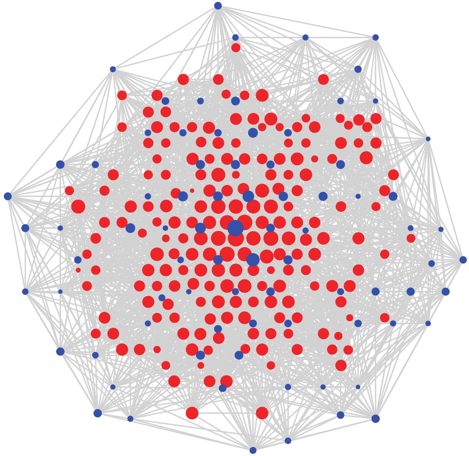
Figure 3. (color online) Graph-structured LHAASO-KM2A detectors activated by a 500-TeV EAS event, where red dots represent EDs, and blue dots represent MDs. Dot size depicts logarithmic scale of recorded photoelectrons.
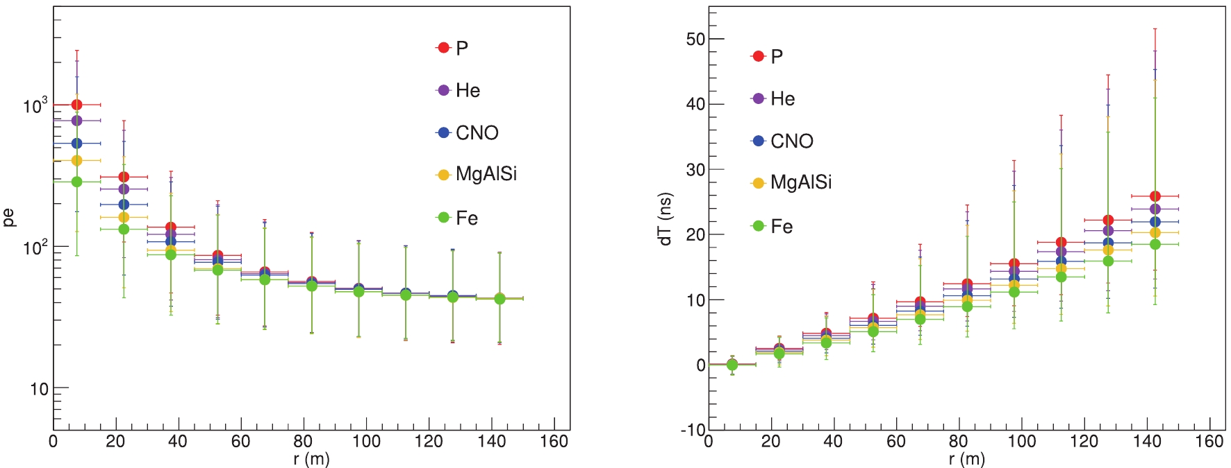
Figure 4. (color online) Relations among three-dimensional vectors. Left panel:
$pe - r$ distribution. Right panel:$dT - r$ distribution. CR groups (P (red), He (violet), CNO (blue), MgAlSi (yellow), Fe (green)) are shown for comparison.$ \begin{array}{l} d_{ij} = {\rm e}^{- \frac12 (\lVert x_i - x_j \rVert - \mu_t)^2 / \sigma_t^2} , \end{array} $

(6) $ \begin{array}{l} a_{ij} = \frac{d_{ij}}{\displaystyle\sum\limits_{k \in N} d_{ik}}. \end{array} $

(7) In Eq. (7),
$ a_{ij} $ is the normalized weight element in the adjacency matrix, and$ N $ represents the set of adjacent detectors with respect to the detector$ i $ . The$ \mu_t $ and$ \sigma_t $ are learnable parameters, which define the locality of the convolutional kernel. In addition, the diagonal elements in the matrix A are set to zero.Before implementing the graph convolution layers, we extract the higher-dimensional features from the input vectors through the learnable function, as shown in Eq. (8), where the
$ n \ \times \ 3 $ vertex matrix$ v $ converts into the$ n \ \times \ d^{(0)} $ matrix$ x^{(0)} $ .$ \begin{array}{l} x^{(0)} = {\rm ReLu}(W^{(0)} v + b^{(0)}). \end{array} $

(8) Then, we define a sequence of T convolution layers, as shown in Eq. (10). Each convolution layer
$ t $ first aggregates the neighbors by multiplication with the adjacency matrix A and expands the vector from$ d^{(t)} $ - to the$ 2 d^{(t)} $ - dimension. Subsequently, the weighting function is applied to update the vector into the$ d^{(t+1)} $ - dimension. The nonlinear activation function$ {\rm ReLu} $ is employed, except in the last convolution layer$ T $ .$ \begin{array}{l} G{\rm Conv}(x^{(t)}) = W^{(t)} [ x^{(t)}, A x^{(t)} ] + b^{(t)}, \end{array} $

(9) $ \begin{array}{l} {x^{(t+1)} = \begin{cases} {\rm ReLu}(G{\rm Conv}(x^{(t)})), & t+1 < T \\ G{\rm Conv}(x^{(t)}), & t+1 = T \end{cases}} \end{array} $

(10) The graph structure is preserved during convolutional operations. In the last convolution layer, i.e., Tth layer, we add a global pooling layer to collect features across the entire graph and compress the graph into a size-invariant representation. The
$ n \times d^{(T)} $ feature matrix is averaged and converted into a$ 1 \times d^{(T)} $ -dimensional matrix. The definition of the global pooling layer is$ \begin{aligned} x_i^{\rm (pool)} = \frac1N \sum\limits_{n \in N} x_{ni}^{(T)}. \end{aligned} $

(11) At the last layer, we employ a linear layer, and the logistic regression is applied to evaluate the event score as the classifier,
$ \begin{array}{l} y = {\rm sigmoid}( W^{\rm (pool)} x^{\rm (pool)} + b^{\rm (pool)} ) , \end{array} $

(12) where
$ x^{\rm (pool)} $ is the$ d^{(T)} $ -dimensional feature from the global pooling layer, and$ y $ is the voting score. The activation function$ {\rm sigmoid} $ ensures that the score y spreads within the range$ [0,1] $ , where the signal-like or background-like event approaches 1 or 0, respectively.We construct the GNNs for ED and MD independently, and fuse their outputs through the linear layer in Eq. (12) with the
$ x^{\rm (pool)} $ as a$ 2d^{(T)} $ -dimensional vector. Independent GNN models for ED and MD are preserved for comparison. The entire GNN architecture is illustrated in Fig. 5.
Figure 5. (color online) KM2A GNN model. Upper red network represents GNN ED model, and lower blue network represents GNN MD model. Right-most rectangle contains the fusion operation of the two models (GNN ED+MD) and their independent outputs.
-
We employ the Monte Carlo simulation to generate event data for training and evaluating KM2A GNN performance. The primary EAS events are generated by the CORSIKA package with the hadronic model QGSJETII [42]. The KM2A detector simulation is performed based on the Geant4 framework [43, 44]. We generate major CR groups including the Proton (P), Helium (He), medium group (CNO), heavy group (MgAlSi), and Iron (Fe). Total events are generated into four energy fragments, including 10 ~ 100 TeV, 100 ~ 1 PeV, 1 ~ 10 PeV, 10 ~ 100 PeV, with the spectral index of –2.7. Reconstructed energies from 100 TeV to 10 PeV are considered, which cover most of the CR knee region. For each task, these groups are divided into independent signal and background groups, where only P belongs to the signal for the P task, and P&He forms the signal for the L task.
After reconstruction of the simulated events [26], we further select events according to their reconstructed locations and directions. The reconstructed shower core spread inside the KM2A array within the distance 200 ~ 500 m from the array center is selected. We ignore the inner circular area (within 200 m) to suppress the disturbance from the WCDA for the KM2A reconstruction. Further, the reconstructed zenith angle below
$ 35^{\circ} $ is also required. Consequently, 105732 events remain for the following analysis. We split the selected events into train, test, and evaluation data sets. In consideration for the data balance, the group ratios for each data set are readjusted to maintain roughly$ 1:1 $ signal-to-noise ratio (SNR). The readjusted data sets for each task are listed in Table 1. The dataset ratio between the two major energy fragments, with 100 TeV ~ 1 PeV and 1 ~ 10 PeV, is around$ 2:1 $ .data set P L signal background signal background train 14635 14595 24358 23733 test 2875 2831 4754 4713 evaluation 24921 22994 24921 22994 Table 1. Number of signal and background events for each dataset.
To train the GNN models, we employ supervised learning techniques with the mean square error (MSE) as the loss function. For each training epoch, the loss is calculated on the test dataset to avoid overfitting. The Adam [45] optimizer is used to optimize the model parameters based on adaptive estimation of low-order moments. The training procedure includes two steps, (i) two independent trainings for the GNN ED and MD models with the learning rate 0.001, and (ii) a subsequent fine-tuning procedure fuses the ED and MD model together with the learning rate 0.0001. It runs over a total of 80 epochs with the model already converged. All code is written in Python using the open-source deep learning framework PyTorch with GPU acceleration. For each model training, four identical candidates with different randomized weights are trained, and the one with the best performance is selected for further processing, which helps suppress the local optimization.
-
We evaluate model performances on the evaluation dataset for each task. Fig. 6 displays the distribution of output scores. All results from the P and L tasks are depicted at the left and right channels, respectively. Intuitively, the shape of the score indicates that the task for classifying the light group is significantly easier than the singular proton group. We calculate the receiver operating characteristic (ROC) curves for explicit comparison. The ROC curves of the physics baseline are integrated on the
$ N_{\mu}/N_e $ distribution, while the curves of the GNN models are integrated on the scores. Results are shown in Fig. 7. The ROC x axis, referred to as the false positive rate, indicates the background retention rate. The ROC y axis, referred to as the true positive rate, indicates the signal efficiency. Fig. 7 clarifies that the best performance is obtained with the fused GNN model, whereas the physics baseline model yields the poorest performance. The ED GNN model performs better than the MD GNN, implying that the sparsity of the sub-array takes the essential effect.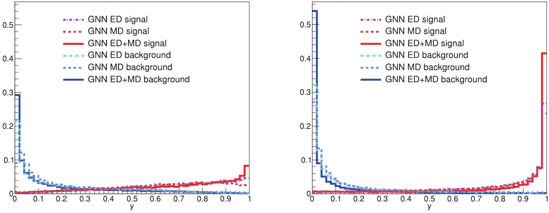
Figure 6. (color online) Distribution of output scores from each model for P task (left) and L task (right).
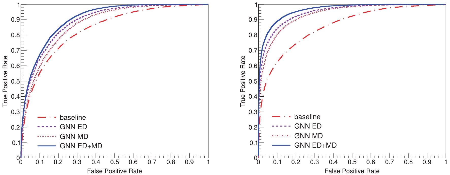
Figure 7. (color online) ROC curves from each model for P task (left) and L task (right).
To reduce the sensitivity to noise due the limited size of the data set and to quantitatively evaluate the model performance, we use the area under the ROC curves (AUC) as a measure of the model performance. We further split the dataset into a sequence of energy bins for comparison of the performance across the entire energy range. We split the energy range withing one order of magnitude into five uniform bins in logarithmic coordinates. The selected events are weighted according to the Horandel model [46] to mimic the actual spectrum for the subsequent analysis. We calculate the AUC values of the models at each bin and plot them in Fig. 8. The results confirm the conclusions announced above. Furthermore, they also show that the fused GNN model outperforms the physics baseline for all energies. We average the AUCs values and list them in Table 2. The fused GNN model achieves the highest score with 0.878 for the P task, and 0.959 for the L task. The AUC score of the L task consistently exceeds the P task by a considerable amount, which is about 0.068 in the physics baseline and rises up to 0.081 in the fused GNN model. Because the nuclear numbers of the Proton and Helium are close, it is difficult to discriminate the Proton from the Helium background.
P L baseline 0.836 0.904 GNN MD 0.847 0.93 GNN ED 0.861 0.936 GNN ED+MD 0.878 0.959 Table 2. Average AUC scores.
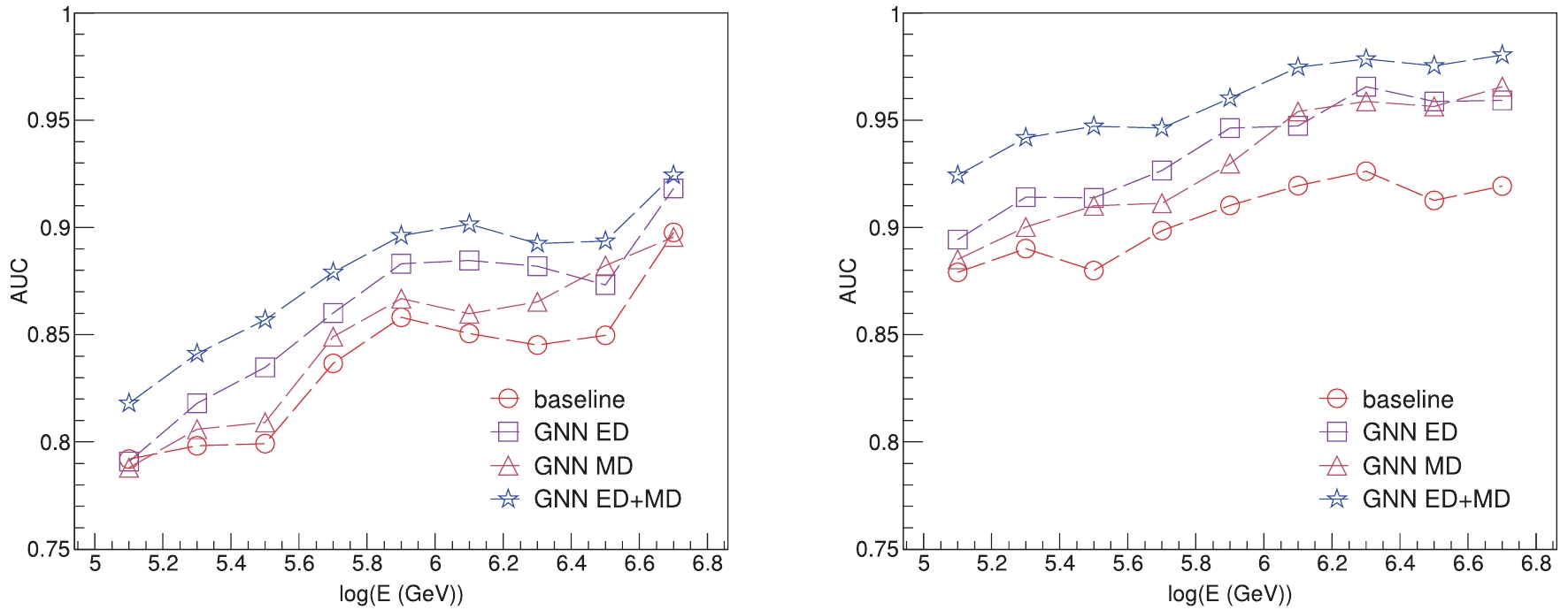
Figure 8. (color online) AUC values across energy range from 100 TeV to 10 PeV from each model for P task (left) and L task (right).
With regard to the real measurement, the significant quantity extracted from the ROC curves is the purity, which is a criterion for subtracting background contamination [22]. The derived purities are shown in Table 3, which are under the same selection efficiency as the LHAASO hybrid detection methods [27,28], for comparison. Results demonstrate that the GNN method yields state-of-art performance among KM2A-only methods and performs comparably to the hybrid detection except for a slight deficiency in the P task. The hybrid detections, including making handcrafted features [27] and the gradient boosted decision tree (GBDT) [28], employ latent representations from WCDA, KM2A, and WFCTA in the LHAASO experiments under stricter selection criteria. This achieves high performance, but causes loss of significant statistics. We also show the apertures of KM2A-only and hybrid detection methods in Table 3. Aperture results are derived from the selection criteria. The KM2A-only methods can achieve an aperture 87× larger than hybrid detections. Considering the WFCTA's strict observation condition with only ~ 10% duty cycle [27], the total statistics of the KM2A are expected to be the on the order of 870× larger than the hybrid detection. We illustrate the expected observation with a one-day operation of the KM2A on the proton- and light-group spectra in Fig. 9, where the rigidity- and mass-dependent knee models are adopted from Refs. [21,47]. As demonstrated in Refs. [21,48], the spectral blur from the measurement maintains the spectral slope and knee position. Hence, the input spectra are adopted as the observation in Fig. 9, with emphasis on the statistical error bars.
Purity (%) (+stat.+sys.) Aperture ( ${\rm m^2 \cdot sr}$ ) (+stat.+sys.)

P L P L handcraft (hybrid) [27] ~90 ~95 ~1.5e3 ~4e3 GBDT (hybrid) [28] ~90 ~97 ~3.6e3 ~7.2e3 baseline (KM2A) 73.4±2.5±2.4 93.20.9±1.1 3.2e5±1.3e3±1.0e4 6.3e5±2.7e3±7.6e3 CNN (KM2A) 75.4±2.5±2.4 93.3±0.9±1.1 3.2e5±1.3e3±1.0e4 6.3e5±2.7e3±7.6e3 GNN MD (KM2A) 77.1±2.3±2.5 95.9±0.6±1.2 3.2e5±1.3e3±1.0e4 6.3e5±2.7e3±7.6e3 GNN ED (KM2A) 82.8±1.9±2.6 96.6±0.6±1.2 3.2e5±1.3e3±1.0e4 6.3e5±2.7e3±7.6e3 GNN ED+MD (KM2A) 84 ±1.9±2.7 98.2±0.4±1.2 3.2e5±1.3e3±1.0e4 6.3e5 ±2.7e3±7.6e3 Table 3. Signal purity and aperture results of each model in LHAASO experiment
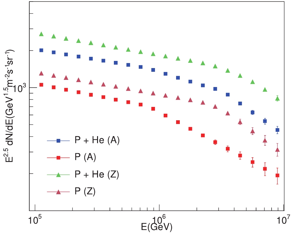
Figure 9. (color online) Expectation on proton- and light-group spectra measured by LHAASO-KM2A with one-day observation. Triangular markers represent spectra predicted by one of the rigidity-dependent knee models (Z) [47], and square markers represent spectra predicted by one of the mass-dependent knee models (A) [21].
We further construct a simple CNN model for comparison with the GNN model. The entire ED and MD arrays are rescaled into regular grids, with
$ (85 \times 97) $ pixels for ED and$ (40 \times 46) $ pixels for MD. Activated detectors are filled into corresponding grids, with others remaining zero. We construct the CNN model with a series of convolution modules for the ED and MD images, and fuse their output together through a linear layer as the classifier. Their performance is shown in Table 3 as well. This demonstrates that the CNN exhibit a poor performance, which we attribute to the insufficient ability in analyzing the large variance of the EAS (10s ~ 1000 activated detectors) and inefficient representation of the image structure (zero grids$ \gtrsim $ 90%). In contrast, because the graph convolutional kernel in Eq. (7) is the Gaussian function with only two learnable parameters (($ \mu_t $ ,$ \sigma_t $ ), while the number of parameters in a CNN convolutional layer is$ C_{\rm out} \times C_{\rm in} \times K_t^2 $ , the training efficiency of the CNN is far less than that of the GNN.To evaluate systematic errors, we further consider the influences from two aspects. The first contribution is the hadronic model, selected for generating the Monte Carlo simulation data. From the reasearch on the LHAASO-KM2A prototype array, this difference between the hadronic models (QGSJETII and EPOS) is roughly 5% with regard to the secondary particles [49]. Hence, we choose a variance of 5% on the recorded
$ pe $ in estimating systematic errors. The resulting errors vary within 2.4% for the P task and 0.4% for the L task. In the actual running of the KM2A experiment, the detector may be randomly dropped, which will then not be fired as the CR event is recorded. As this type of effect does not occur in the simulation, this will introduce systematic errors in the inference of the real data. Supposing that the detectors may drop 5% in the actual running, we randomly drop them from the fired detectors on the simulation data and re-evaluate the model performance. The results shows that this effect causes errors of aproximately 2.1% for the P task and 1.1% for the L task. The analysis demonstrates the stability of the GNN method. Both the evaluation of statistical and systematic errors are shown in Table 3. In future studies, when the LHAASO experimental data is acquired, a detailed comparison between the simulation and real data is necessary for estimating other systematical errors. -
Deep learning has contributed extensively to significant progress in numerous fields. Therefore, we leverage this technology to improve classification performance in the LHAASO -KM2A experiment. We propose a fused GNN model, which constructs independent networks for the KM2A ED and MD arrays, and fuse their outputs for classification. This model is demonstrated to be effective, and its performance outperforms the traditional physics-based method as well as the CNN-based method over the entire energy range. Furthermore, we compare the performance of the GNN framework for independent ED and MD arrays. The ED array is found to behave better than the MD array. We attribute this to the higher density configuration of the ED array. Moreover, in comparison with the LHAASO hybrid detection method, our KM2A GNN model exhibits competitive classification performance. Owing to the large area and full duty cycle of the KM2A array, it can acquire statistics on the order of ~ 870× higher than the hybrid detection.
We thank the LHAASO Collaboration for their support on this project.
Classifying cosmic-ray proton and light groups in LHAASO-KM2A experiment with graph neural network
- Received Date: 2019-11-05
- Accepted Date: 2020-02-16
- Available Online: 2020-06-01
Abstract: The precise measurement of cosmic-ray (CR) knees of different primaries is essential to reveal CR acceleration and propagation mechanisms, as well as to explore new physics. However, the classification of CR components is a difficult task, especially for groups with similar atomic numbers. Given that deep learning achieved remarkable breakthroughs in numerous fields, we seek to leverage this technology to improve the classification performance of the CR Proton and Light groups in the LHAASO-KM2A experiment. In this study, we propose a fused graph neural network model for KM2A arrays, where the activated detectors are structured into graphs. We find that the signal and background are effectively discriminated in this model, and its performance outperforms both the traditional physics-based method and the convolutional neural network (CNN)-based model across the entire energy range.


 DownLoad: